People re-identification using deep appearance, feature and attribute learning

(1)

warwick.ac.uk/lib-publications

A Thesis Submitted for the Degree of PhD at the University of Warwick

Permanent WRAP URL:

http://wrap.warwick.ac.uk/144567

Copyright and reuse:

This thesis is made available online and is protected by original copyright.

Please scroll down to view the document itself.

Please refer to the repository record for this item for information to help you to cite it.

Our policy information is available from the repository home page.

(2)

People Re-identification using

Deep Appearance, Feature and

Attribute Learning

by

Gregory Watson

Thesis

Submitted to the University of Warwick for the degree of

Doctor of Philosophy in Urban Science

Department of Computer Science

(3)

List of Tables

3.1 The dimensionality of each of the feature type used in our experi-mentation. Due to the higher resolution available for most images within the CUHK03 [111] data set, we resize to 160_⇥60 pixels for LOMO and Weighted LOMO feature extraction, rather than 128⇥48 pixels, resulting in a higher dimensional feature descriptor. . . 70 3.2 The VIPeR [59] data set was split into two sets, with 316 identities

allocated for training and 316 for testing. Every probe image in the test set is compared to every gallery image in the test set. PLSAM(v2) consists of the Weighted LOMO and limb-by-limb level SCNCD feature descriptors with XQDA, whereas PLSAM(v1) consists just of the Weighted LOMO feature descriptors with XQDA. . . 76 3.3 The QMUL GRID [117, 124, 125] data set was split into two sets,

with 125 identities allocated for training and 900 for testing. The 900 testing identities consisted of 125 image pairs and 775 single images. Every probe image in the test set is compared to every gallery image in the test set. PLSAM(v2) consists of the Weighted LOMO and limb-by-limb level SCNCD feature descriptors with XQDA, whereas PLSAM(v1) consists just of the Weighted LOMO feature descriptors with XQDA. . . 82 3.4 The CUHK03 [111] data set was split into two sets, with 1160 identities

allocated for training and 100 for testing. Every probe image in the test set is compared to every gallery image in the test set. PLSAM(v2) consists of the Weighted LOMO and limb-by-limb level SCNCD feature descriptors with XQDA, whereas PLSAM(v1) consists just of the Weighted LOMO feature descriptors with XQDA. . . 84

(7)

4.1 Results on the VIPeR [59] data set. The best results are highlighted in bold. (v1) refers to the Weighted LOMO features and XQDA, whereas (v2) refers to the Weighted LOMO features with the limb-by-limb level SCNCD features and XQDA. . . 100 4.2 Results on the QMUL GRID [117, 124, 125] data set. The best results

are highlighted in bold. (v1) refers to the Weighted LOMO features and XQDA, whereas (v2) refers to the Weighted LOMO features with the limb-by-limb level SCNCD features and XQDA. . . 109 4.3 Results on the CUHK03 [111] data set. The best results are shown in

bold. (v1) refers to the Weighted LOMO features and XQDA, whereas (v2) refers to the Weighted LOMO features with the limb-by-limb level SCNCD features and XQDA. . . 111 5.1 Attribute detection accuracy on the VIPeR [59] data set. The ten

best and worst attributes detection accuracies are shown. . . 120 5.2 Results on the VIPeR [59] data set. The best results are highlighted

in bold. Results marked with * do not incorporate attribute features. 123 5.3 Results on the PRID2011 [70] data set. The best results are highlighted

in bold. Results marked with * do not incorporate attribute features. 124 5.4 Results on the i-LIDS [57, 225, 226] data set. The best results are

high-lighted in bold. Results marked with * do not incorporate attribute features. . . 125 5.5 Results on the Market-1501 [219] data set. The best results are

high-lighted in bold. Results marked with * do not incorporate attribute features. . . 126 5.6 Results on the VIPeR [59] data set utilising di↵erent combinations of

the original and parts-based images. Models are trained with BCE loss. The best results are highlighted in bold. . . 127 5.7 Results on the VIPeR [59] data set utilising WBCE loss and BCE

loss. The best results are highlighted in bold. . . 130 5.8 Results on the PRID2011 [70] data set utilising WBCE loss and BCE

loss. The best results are highlighted in bold. . . 130 5.9 Results on the i-LIDS [57, 225, 226] data set utilising WBCE loss and

BCE loss. The best results are highlighted in bold. . . 131 5.10 Results on the Market-1501 [219] data set utilising WBCE loss and

BCE loss. The best results are highlighted in bold. . . 131 5.11 The cosine distance between the attribute distribution of the training

(8)

List of Figures

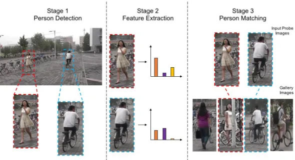
1.1 An example of the three stages of Re-ID. In stage 1, the person is localised from within the image frame. In stage 2, feature descriptors are extracted from each image. In stage 3, each input probe image is matched with the gallery image the smallest distance away in the feature space. Images with the same colour outline are of the same identity. Examples are taken from the PRW [223] data set. . . 2 1.2 Example images from Re-ID data sets [6–8, 57, 59, 70, 117, 125, 225,

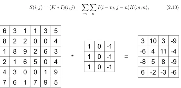
226]. Each column represents a single identity. All images have been scaled to a standard resolution. . . 2 2.1 An example of the convolution operation applied on a 6 _⇥6 matrix

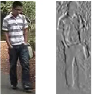
with a 3_⇥ 3 filter. . . 15 2.2 An example of the 3⇥3 filter in Figure 2.1 applied to an image. It can

be observed that the filter highlights vertical edges within the image. In CNNs, the weights of the filter are learned by backpropagation. . 16 2.3 An example of max-pooling used to downsample a feature map. Within

each pooling region, represented by a distinct colour, the maximum value is taken to form the corresponding value in the output feature map. . . 17 2.4 An example of average-pooling used to downsample a feature map.

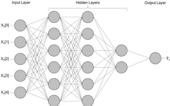
Within each pooling region, represented by a distinct colour, the average value of all values is taken to form the corresponding value in the output feature map. . . 17 2.5 A simple network containing only fully-connected layers. The network

(9)

2.6 A typical use-case for a CNN within the field of Re-ID. A pedestrian image from the VIPeR [59] data set is passed as input to a CNN, and is passed through a series of hidden layers to create a series of feature maps. Once the final feature map has been computed, it is passed to a fully-connected layer, where each unit within the fully-connected layer represents an identity. In this example, the network has predicted with 74% confidence that the identity of the person present in the

input image is ID2. . . 19

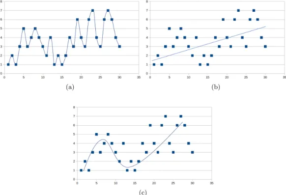
2.7 Examples of (a) overfitting, (b) underfitting and (c) achieving a good fit on a data set. . . 23

(a) . . . 23

(b) . . . 23

(c) . . . 23

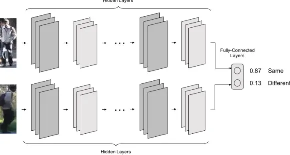
2.8 An example of a network trained using Verification Loss. The network is trained to predict whether or not a given pair of images represent the same identity or otherwise. The example images are taken from the VIPeR [59] data set. . . 25

2.9 An example of a network trained using ID Classification Loss. The network is trained to predict the identity of a given image. The example image is taken from the VIPeR [59] data set. . . 26

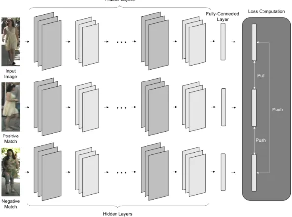
2.10 An example of a deep neural network utilising triplet loss. Three images are passed to the network, an input image, apositive match image with the same identity as the input image, and anegative match with a di↵erent identity to the input and positive match images. The networkpulls the output of the input and positive match to be closer, by minimising the distance between the two within the output feature space. Furthermore, the network pushes the input and positive match away from the negative match, by maximising the distance between the di↵erent identities within the output feature space. . . 29

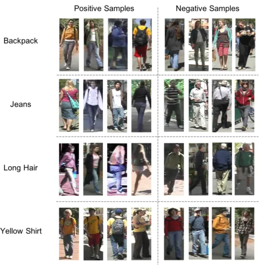
2.11 Example attributes and corresponding positive and negative examples. Images are taken from the VIPeR [59] data set with attribute labellings taken from the PETA [39] data set. . . 34

(10)

2.12 A comparison between rank-nand mAP/AP. It can be observed that whilst the rank-1 rate is consistently 100% throughout all examples, utilising mAP and AP better evaluates the performance when multiple images of the same identity as the input probe image are present within the gallery set. Images with the same identity as the input probe image are highlighted in green, whereas images with a di↵erent identity are highlighted in red. All images are from the Market-1501 [219] data set. 40 2.13 Example images from the VIPeR [59] data set. Each column represents

a single identity. All images have been scaled to a standard resolution. 41 2.14 Example images from the QMUL GRID [117, 124, 125] data set. Each

column represents a single identity. All images have been scaled to a standard resolution. . . 42 2.15 Example images from the CUHK01 [110] data set. Each column

represents a single identity. All images have been scaled to a standard resolution. . . 43 2.16 Example images from the PRID2011 [70] data set. Each column

represents a single identity. All images have been scaled to a standard resolution. . . 43 2.17 Example images from the 3DPeS [6–8] data set. Each column

rep-resents a single identity. All images have been scaled to a standard resolution. . . 44 2.18 Example images from the i-LIDS [57, 225, 226] data set. Each column

represents a single identity. All images have been scaled to a standard resolution. . . 44 2.19 Example images from the Market-1501 [219] data set. Each column

represents a single identity. All images have been scaled to a standard resolution. . . 45 2.20 Example images from the DukeMTMC-reID [152, 228] data set. Each

column represents a single identity. All images have been scaled to a standard resolution. . . 46 2.21 Example images from the PETA [39] data set. All images have been

scaled to a standard resolution. Individual images are originally part of [6–8, 12–14, 29, 57, 59, 70, 109–111, 117, 125, 142, 225, 226]. . . . 47 3.1 Examples of our PLS skeleton fitting on images from the VIPeR [59]

data set. Each set of five images contains: the original image, the input HOG appearance features, the ground-truth skeleton keypoints, our predicted skeleton using the PLS regression model and the foreground image mask. . . 55

(11)

3.2 Examples of orientation groups from the VIPeR [59] data set. For this data set, we split the images into two orientation groups: those facing perpendicular (90°) to the camera, and those facing all other directions relative to the camera. . . 56 3.3 Examples of training the PLS appearance model on di↵erent subsets

of the VIPeR [59] data set. The third column shows training only on images containing people with non-perpendicular orientations relative to the camera. The fourth column represents training on images con-taining only images concon-taining people with perpendicular orientations relative to the camera. The fifth and final column shows training on images containing people with all poses relative to the camera. It can be seen that the lowest RMSE is obtained by training on images with similar orientations to the input image. . . 58 3.4 Example image pairs from the VIPeR [59] data set, containing both

the original images as well as the images after the Retinex preprocesing step has been applied. . . 62 3.5 The LOMO [115] feature extraction method. The diagram is based

on a similar diagram contained in [115]. . . 64 3.6 SCNCD [208] feature extraction at a limb-by-limb level. The

his-tograms below each individual limb image represent the extracted feature descriptor, with each bar representing an individual colour name. . . 66 3.7 Our proposed method for weighting the LOMO feature descriptor.

Patch features are extracted from each 10_⇥10 pixel region, and then weighted by multiplying by the percentage of foreground pixels. Then, we take all patches in the same horizontal location and use the maximum value of each bin to contribute towards the final feature descriptor for that horizontal location. . . 68 3.8 Examples of ground-truth and predicted skeletons from the VIPeR [59]

data set. The average RMSE over the entire test set is 5.2 pixels. . . 71 3.9 The distribution of RMSE on skeletons predicted by the PLS-based

skeleton prediction model on the VIPeR [59] data set. . . 72 3.10 Examples of ground-truth skeletons, and skeletons predicted using our

PLS model on the VIPeR [59] data set which achieves a good skeleton fitting result. . . 73 3.11 Examples of ground-truth skeletons, and skeletons predicted using our

PLS model on the VIPeR [59] data set which achieves a poor skeleton fitting result. . . 74

(12)

3.12 CMC on the VIPeR [59] data set. All of our CMC curves are single-shot results. Results are reproduced from [115], [217], [212], [111] and [113]. . . 76 3.13 Examples of ground-truth and predicted skeleton from the QMUL

GRID [117, 124, 125] data set. The average RMSE over the entire test set is 5.3 pixels. . . 78 3.14 The distribution of RMSE on skeletons predicted by the PLS-based

skeleton prediction model on the QMUL GRID [117, 124, 125] data set. 79 3.15 Examples of ground-truth skeletons, and skeletons predicted using

our PLS model on the QMUL GRID [117, 124, 125] data set which achieves a good skeleton fitting result. . . 80 3.16 Examples of ground-truth skeletons, and skeletons predicted using

our PLS model on the QMUL GRID [117, 124, 125] data set which achieves a poor skeleton fitting result. . . 81 3.17 CMC on the QMUL GRID [117, 124, 125] data set. All of our CMC

curves are single-shot results. Results are reproduced from [115], [217], [212], [111] and [113]. . . 82 3.18 CMC on the CUHK03 [111] data set. All of our CMC curves are

single-shot results. Results are reproduced from [115], [217], [212], [111] and [113]. . . 84 4.1 The network architecture for our proposed deep foreground modelling

network. We first rescale images to a resolution of 224⇥224 pixels, and pass the images through the convolutional layers of a ResNet-50 network [66]. We take the POOL5 average pooling layer as the output of the ResNet-50 model, flatten the output, and pass the output through two further fully-connected layers. The output of our proposed network contains 58 units, representing the (x, y) coordinates of the skeleton key-points (joints and edge markers). We use the RMSProp [177] optimizer, with a mean squared error loss. . . 89 4.2 Examples of images, skeletons, and their corresponding augmentations.

The first image in each row is the original image. The remaining images in each row are augmentations of the first image. . . 90 4.3 Examples of ground-truth, skeletons predicted using our deep model,

and skeletons predicted using our PLS model on the VIPeR [59] data set. The average RMSE when using the deep model was 4.5 pixels, whilst the average when using the PLS model was 5.2 pixels. . . 93

(13)

4.4 The distribution of RMSE on skeletons predicted by the deep skeleton prediction model on the VIPeR [59] data set. The average RMSE was 4.5 pixels, whilst the average using the PLS model was 5.2 pixels. . . 94 4.5 Examples of ground-truth, skeletons predicted using our deep model,

and skeletons predicted using our PLS model on the VIPeR [59] data set which achieve a good skeleton fitting result. . . 95 4.6 Examples of ground-truth, skeletons predicted using our deep model,

and skeletons predicted using our PLS model on the VIPeR [59] data set which achieve a poor skeleton fitting result. . . 96 4.7 A comparison of skeleton fitting results using our deep method against

the fittings labelled as poor in Figure 3.11. . . 97 4.8 Further comparisons of skeleton fitting results using our deep method

against the fittings labelled as poor in Figure 3.11. . . 98 4.9 CMC on the VIPeR [59] data set. All of our CMC curves are single-shot

results. Results are reproduced from [77, 111, 113, 115, 189, 212, 217]. 101 4.10 Examples of ground-truth, skeletons predicted using our deep model,

and skeletons predicted using our PLS model on the QMUL GRID [117, 124, 125] data set. The average RMSE when using the deep model was 5.5 pixels, whilst the average when using the PLS model was 5.3 pixels. . . 103 4.11 The distribution of RMSE on skeletons predicted by the deep skeleton

prediction model on the QMUL GRID [117, 124, 125] data set. The average RMSE was 5.5 pixels, whilst the average using the PLS model was 5.3 pixels. . . 104 4.12 Examples of ground-truth, skeletons predicted using our deep model,

and skeletons predicted using our PLS model on the QMUL GRID [117, 124, 125] data set which achieve a good skeleton fitting result using our deep model. . . 105 4.13 Examples of ground-truth, skeletons predicted using our deep model,

and skeletons predicted using our PLS model on the QMUL GRID [117, 124, 125] data set which achieve a poor skeleton fitting result using our deep model. . . 106 4.14 A comparison of skeleton fitting results using our deep method against

the fittings labelled as poor in Figure 3.16. . . 107 4.15 Further comparisons of skeleton fitting results using our deep method

(14)

4.16 CMC on the QMUL GRID [117, 124, 125] data set. All of our CMC curves are single-shot results. Results are reproduced from [77, 111, 113, 115, 189, 212, 217]. . . 109 4.17 CMC on the CUHK03 [111] data set. All of our CMC curves are

single-shot results. Results are reproduced from [77, 111, 113, 115, 189, 212, 217]. . . 112 5.1 An example of images from the VIPeR [59] data set. All of these

images are labelled as wearing blue clothing on their upper bodies by the PETA [39] data set. However, significant visual variation can be seen between images, such as pose and illumination variation. . . 116 5.2 An example of how we divide each Re-ID image into three parts-based

images: top, middle and bottom, using our deep CNN-based method proposed in Chapter 4. We create a bounding box around each part, and add padding of 15% in thex and y dimensions, to account for any errors in skeleton prediction. We use the original image and the three parts-based images as input to our attribute prediction model. (a) The original input image; (b) The original image with the skeleton and parts separation overlayed; (c) The individual body parts images. 118 5.3 The network architecture of the attribute prediction model. The

original image is divided into three body parts - the top, middle and bottom. The original image, as well as the three body parts images, are passed through an identical ResNet-50 [66] network architecture. The fully-connected layers of each ResNet-50 model are removed and replaced with our own fully-connected layer of size 512. The four fully-connected layers are then concatenated to form a layer of size 2048. Finally, we append a fully-connected layer of size n, with n

being the number of attributes being predicted. . . 119 5.4 Examples of attribute prediction accuracy. All images shown in

(a) are predicted to be wearing red clothing on their upper body, whilst images in (b) are predicted to be wearing a backpack. Images correctly classified (true-positive) are highlighted in green, whilst those incorrectly classified (false-positive) are highlighted in red. The predicted probability of the presence of each attribute is shown below each image. . . 121 5.5 The distribution of attributes on the data sets used to train the

attribute model, versus the three data sets used to evaluate the attribute model. . . 132

(15)

A.1 Example images and their corresponding hand-labelled skeletons from the VIPeR [59] data set. . . 143 A.2 An example of the skeleton labelling GUI using images from the

VIPeR [59] data set. The first Re-ID image represents the input image on which the user clicks to mark skeleton keypoints. The second Re-ID image shows the recorded skeleton keypoints converted to a skeleton and overlayed on the input image in real-time. The third image is a static reference image showing the order in which the skeleton keypoint should be collected. Finally, some information on the Re-ID image is shown on the right of the GUI. . . 144

(16)

Acknowledgments

Firstly, I would like to express my sincere gratitude to my supervisor, Dr. Abhir Bhalerao, for the continuous support that he has provided throughout my study. I have benefited greatly from his encouragement and advice, as well as with his immense knowledge and experience. I would also like to thank Dr. Matthew Leeke and Prof. Nasir Rajpoot for acting as advisors throughout the project.

Furthermore, I would like to thank my friends and colleagues in the Warwick Institute for the Science of Cities and Department of Computer Science, Katherine Ascott, Jamie Bayne, Matthew Bradbury, James Van Hinsbergh, Melissa Kenny, Richard Kirk, Helen McKay, David Purser, John Rahilly, Liam Steadman, David Truby and Ian Tu for the support, laughs and great times that we shared. I would additionally like to thank the support sta↵, Yvonne Colmer, Katie Martin and Jenny Eborall, who have helped significantly over the past years with support and organisational matters.

Lastly, I would like to thank my family and Andrew Brooks, for their support and encouragement throughout my PhD study.

(17)

Declarations

I declare that the work presented in this thesis, titledPerson Re-identification using

Deep Appearance, Feature and Attribute Learning, is original work, and has not

been submitted for a degree at another university. Parts of this thesis have been previously published in the following:

• Gregory Watson and Abhir Bhalerao. Person re-identification using partial least squares appearance modelling. InInternational Conference on Image Analysis

and Processing, pages 25–36. Springer, 2017. doi: 10.1007/978-3-319-68548-9 3

• Gregory Watson and Abhir Bhalerao. Person reidentification using deep foreground appearance modeling. Journal of Electronic Imaging, 27(5):051215, 2018. doi: 10.1117/1.JEI.27.5.051215

• Gregory Watson and Abhir Bhalerao. Person re-identification combining deep features and attribute detection. Multimedia Tools and Applications, December 2019. doi: 10.1007/s11042-019-08499-9

(18)

Abstract

Person Re-Identification (Re-ID) is the act of matching one or more query images of an individual with images of the same individual in a gallery set. We propose various methods to improve Re-ID performance via foreground modelling, skeleton prediction and attribute detection.

Foreground modelling is an important preprocessing step in Re-ID, allowing more representative features to be extracted. We propose two foreground modelling methods which learn a mapping between a set of training images and skeleton keypoints. The first utilises Partial Least Squares (PLS) regression to learn a mapping between Histogram of Oriented Gradients (HOG) features extracted from person images, and skeleton keypoints. The second instead learns the mapping using a deep convolutional neural network (CNN). Using a CNN has been shown to generalise better, particularly for unusual pedestrian poses.

We then utilise the predicted skeleton to generate a binary mask, separating the foreground from the background. This is useful for weighting image features extracted from foreground areas higher than those extracted from background areas. We apply this weighting during the feature extraction stage to increase matching rates.

The predicted skeleton can be used to divide a pedestrian image into multiple parts, such as head and torso. We propose using the divided images as input to an attribute prediction network. We then use this network to generate robust feature descriptors, and demonstrate competitive Re-ID matching rates.

We evaluate on a number of di↵erent Re-ID data sets, each possessing signi-ficant variations in visual characteristics. We validate our proposals by measuring the rank-n score, which is equivalent to the percentage of identities correctly pre-dicted withinnattempts. We evaluate our skeleton prediction network using root mean square error (RMSE), and our attribute prediction network using accuracy. Experiments demonstrate that our proposed methods can supplement traditional Re-ID approaches to increase rank-nmatching rates.

(19)

Acronyms

AP Average Precision.

AUC Area Under The Curve.

BCE Binary Cross-Entropy.

CAN Comparative Attention Network.

CCA Canonical Correlation Analysis.

CCE Categorical Cross-Entropy.

CMC Cumulative Matching Characteristic.

CNN Convolutional Neural Network.

CPS Custom Pictorial Structures.

CRF Colour Restoration Function.

DFAD Deep Features & Attribute Detection.

DGD Domain Guided Dropout.

DNAM Deep Network Appearance Model.

DPM Deformable Part Model.

FAN Feature Aggregation Network.

FN False Negative.

FP False Positive.

FPNN Filter Pairing Neural Network.

GAN Generative Adversarial Network.

(20)

GUI Graphical User Interface.

HOG Histogram of Oriented Gradients.

IBP Indian Bu↵et Process.

JLML Jointly Learning Multi-Loss.

LNCC Local Normalized Cross-Correlation.

LOMO Local Maximal Occurrence.

LRN Local Response Normalization.

LSR Label Smoothing Regularization.

LSRO Label Smoothing Regularization for Outliers.

LSTM Long Short-Term Memory.

MAE Mean Absolute Error.

mAP Mean Average Precision.

MLP Multilayer Perceptron.

MLR Multiple Linear Regression.

MSCR Maximally Stable Color Regions.

MSE Mean Squared Error.

MTL Multi-Task Learning.

OLS Ordinary Least Squares.

PCA Principal Component Analysis.

PCR Principal Component Regression.

PLS Partial Least Squares.

PLSAM Partial Least Squares Appearance Model.

PRDC Probabilistic Relative Distance Comparison.

PS Pictorial Structures.

(21)

Re-ID Person Re-Identification.

RHSP Recurrent High-Structured Patches.

RMSE Root Mean Squared Error.

RNN Recurrent Neural Network.

ROC Receiver Operating Characteristic.

SCA Stel Component Analysis.

SCNCD Salient Color Names Based Color Descriptor.

SIFT Scale-Invariant Feature Transform.

SILTP Scale Invariant Local Ternary Pattern.

SURF Speeded-Up Robust Features.

SVD Singular Value Decomposition.

SVM Support Vector Machine.

TN True Negative.

TP True Positive.

WBCE Weighted Binary Cross Entropy.

(22)

Chapter 1

Introduction

Person Re-Identification (Re-ID) is the process of automatically identifying and matching di↵erent images of people taken from separate, non-overlapping cameras at di↵erent times. It has a multitude of important applications in security, surveillance and biometrics, as well as in tracking and people-monitoring.

Re-ID can be broken down into three stages. The first step is to localise the person within the image of the environment, typically by using either a pedestrian detector [111, 219, 220, 224] or via hand-labelling [59, 111, 117, 125, 219]. The second part concerns extracting a robust feature descriptor of the person. A lack of high-resolution imagery in Re-ID data sets have rendered more traditional biometric approaches such as facial recognition unsuitable, leaving low level features either pre-specified by the user, such as colour [43, 58, 115, 117, 130, 148, 208, 216] or texture [43, 58, 115, 117], or those learnt via a deep convolutional neural network (CNN) [2, 27, 28, 51, 90, 108, 111, 112, 200, 203, 206, 229, 230]. The third and final part relates to matching [115, 156, 185, 206, 212], where the distance between the extracted feature descriptors is computed. Whilst some techniques calculate the Euclidean distance between these feature descriptors, this distance metric is often learnt through supervised learning. Given two feature descriptors extracted from di↵erent images of the same person, it is expected that the distance between the two is smaller than the distance between two features descriptors extracted from di↵erent people. An illustrative example of the three stages of Re-ID can be seen in Figure 1.1.

However, Re-ID is often challenging due to the variations in pose, illumination and image resolution caused by the use of distinct, non-overlapping cameras [24, 53, 188]. The extracted feature descriptors are often not invariant to the significant inter-class and intra-class variations often present in Re-ID images. Figure 1.2 shows examples of images from various common Re-ID data sets, and demonstrates the

(23)

Figure 1.1: An example of the three stages of Re-ID. In stage 1, the person is localised from within the image frame. In stage 2, feature descriptors are extracted from each image. In stage 3, each input probe image is matched with the gallery image the smallest distance away in the feature space. Images with the same colour outline are of the same identity. Examples are taken from the PRW [223] data set.

types of variation found in these images.

One of the ways in which the negative e↵ects of variations in visual charac-teristics can be minimised is to pose normalise the images. A significant variation between images is the pose of the person, with some people having been photographed from the front, whilst others have been photographed from the side. Furthermore, across images, limbs such as arms and legs can be located in a wide variety of positions relative to the torso. The variance in the position of a persons body is directly linked to the variation in the position of the background, largely redundant information which is not representative of the person.

One of the ways in which pose and background variation can be minimised is to use a foreground appearance model, built using a model-based approach such as Partial Least Squares (PLS) [127, 155] regression. Utilising this technique, a regression can be learnt between image appearance features, as well as landmarks representing foreground regions of a Re-ID image.

Inspired by the processes of the human brain, an alternative approach is to use methods to learn the optimal mapping between image appearance and foreground landmarks. A specific branch of machine learning, known as deep learning [55, 95, 160], achieves this by using an artificial neural network, which consist of a series of hierarchical layers, including input, output, and “hidden” layers

(24)

Figure 1.2: Example images from Re-ID data sets [6–8, 57, 59, 70, 117, 125, 225, 226]. Each column represents a single identity. All images have been scaled to a standard resolution.

performing operations such as convolution and pooling. Each layer is connected to the next with a series of weights. During training, the network predicts the corresponding output for each input image, and compares its prediction to the ground-truth labels. The network then adjusts its layer weights based on its prediction performance relative to the ground-truth labelling, with the overall goal being to reduce the loss.

However, significantly more training data is required to train a deep neural network compared to more traditional, less complex methods such as PLS. Yet, Re-ID data sets are small in size, with very few images per identity. Furthermore, Re-ID data sets with foreground labelling are uncommon, with most data sets simply consisting of an image and identity labelling. Therefore, training a deep neural network only on Re-ID data sets is often not the best way to achieve a high-performing network. It is commonplace for networks to instead by trained on a problem from a di↵erent domain, such as object recognition, with transfer learning [147] then used to apply the learnt knowledge to the problem of Re-ID. For example, the ResNet-50 [66] network trained on the ImageNet [38] data set is often used as a basis for networks involved in the field of Re-ID.

In this thesis, we focus on the task of minimising the e↵ects of pose and background variations through the use of person appearance modelling, which is a form of foreground modelling. By learning the foreground, we are able to predict the skeleton of an individual when presented with their image. This information can then be used to address specifically the issue of pose variation by providing context to our feature extraction process. We begin with skeleton prediction through

(25)

utilising a PLS-based [127, 155] model. We then employ end-to-end learning to train a CNN to perform the skeleton prediction task. Finally, we combine our skeleton prediction models with attribute information to improve feature engineering, creating features which are more invariant to variations in visual characteristics. We use these techniques to supplement and improve existing Re-ID techniques to increase matching rates, and validate our work on standard Re-ID data sets.

1.1 Methods and Contributions

We make three contributes within this thesis. Two contributions relate to improving feature extraction by assimilating foreground information learnt via a skeleton prediction model, whilst the third relates to improving Re-ID matching rates by incorporating feature descriptors learnt through an attribute prediction method.

1.1.1 Partial Least Squares Appearance Modelling

We propose a novel skeleton prediction method using PLS regression, which learns a mapping between image appearance information and skeleton keypoints. By predicting skeleton information for a given image, we can exploit this information during the feature extraction stage to prioritise feature descriptors extracted from foreground regions. We alter Local Maximal Occurrence (LOMO) [115] features to create Weighted LOMO, which weights LOMO feature descriptors extracted from foreground areas higher than those extracted from background areas. We concatenate with Salient Colour Names Based Colour Descriptor (SCNCD) [208] feature descriptors extracted on a limb-by-limb level, and follow by utilising the Cross-view Quadratic Discriminant Analysis (XQDA) [115] Distance Metric Learning technique to calculate the distance between feature descriptors.

1.1.2 Deep Foreground Appearance Modelling

Following on from the previous work using PLS to learn a mapping between image appearance information and skeleton keypoints, we propose the replacement of the PLS method with a deep CNN. Whilst the PLS approach struggles to handle person images taken from di↵erent angles, and thus requires multiple models to be trained, the Deep CNN approach is able to predict the skeleton of person images with di↵erent poses with a greater degree of accuracy, whilst only requiring a single skeleton prediction model to be trained. Furthermore, we find that our deep CNN-based method is able to better handle the individuals with more unusual poses, such as those with arms raised. We validate the predicted skeletons in a Re-ID framework, and show improvement in matching rates.

(26)

1.1.3 Combining Deep Features and Attribute Detection for Re-ID

We present a CNN-based architecture which takes as input a person image, as well as three parts-based images generated via our Deep Network Appearance Model, and predicts a set of fifty attributes. We then use the penultimate layer in the network as a feature descriptor for matching. Notably, none of the data sets which we use to evaluate our method contribute training images to the attribute network, demonstrating our method’s ability to generalise between di↵erent data sets. Furthermore, given that some attributes will be more prevalent than others within the training set, we propose a novel Weighted Binary Cross Entropy function that weights the cost of a positive error relative to a negative error, based on the ratio of positive to negative instances of each attribute. We evaluate the combined approach on a set of standard data sets.

1.2 Thesis Outline

In Chapter 2, we perform a review of the literature related to Re-ID. We review approaches which utilise spatial & foreground modelling, hand-crafted features, as well as attribute learning. We also detail metrics used to evaluate Re-ID methods, as well as the data sets on which they are evaluated. In Chapter 3, we describe our method which utilises PLS regression to learn a mapping between image appearance information and skeleton keypoints, allowing feature descriptors to be extracted primarily from foreground regions prior to matching. In Chapter 4, we replace our PLS-based skeleton prediction model with a deep CNN-based approach, and compare both the PLS and CNN-based methods. In Chapter 5, we propose utilising skeleton information as context to an attribute prediction network, which is then used as a feature extraction network for matching. Finally, in Chapter 6, we summarise our proposed methods and describe potential future research directions.

(27)

Chapter 2

Literature Review

In this chapter, we discuss and review previous Re-ID techniques, paying particular attention to spatial modelling, feature extraction, deep learning, attribute detection, distance metric learning, and the use of generative adversarial networks.

2.1 Spatial & Foreground Modelling for Re-ID

High accuracy Re-ID results depend on the ability to produce robust feature descriptors which possess low intra-class variation and high inter-class variation, and so, the feature extraction stage is of vital importance. However, extracting feature descriptors from images without attention given to significant background di↵erences can lead to the extracted feature descriptors being a↵ected by extraneous and un-representative background information. Much study [29, 43, 108, 135, 136, 172, 199, 215, 222] has therefore been carried out to investigate methods for separating the foreground from the background, allowing feature descriptors to be extracted either in full or primarily from foreground areas rather than background areas.

Stel Component Analysis [86] (SCA) has been utilised to separate the fore-ground of person images from the backfore-ground. SCA attempts to capture the structure of an image by separating the image into a series of parts, orstels, that possess a similar feature distribution, such as colour or texture. However, if a single part of an image possesses a wide feature distribution, or if two parts of an image possess a similar feature distribution, separation into distinct parts may fail. Farenzena et al. [43] incorporate SCA and divide each person image into three distinct parts according to the person’s limbs, calculating the vertical central axis for each part, and weighting each pixel dependent on the distance to the vertical central axis via a Gaussian kernel. This generally works well given that the pixels closer to a person’s vertical central axis are much more likely to belong to their body, however this may fail if a person has their legs spread widely apart.

(28)

Spatial and foreground modelling can also help counter the problems of pose variation. Extracting feature descriptors without paying due attention to pose variations between images can lead to lack of spatial correspondence between the extracted feature descriptors. In Local Maximal Occurrence (LOMO) [115], the authors extract a histogram-based feature descriptor from 10⇥10 pixel patches, with an overlap of 5 pixels in each dimension. For each row of feature descriptors extracted, they take the maximum value in each histogram bin to form the final feature descriptor for that row. Whilst not explicitly removing or deprioritising the background information like alternative methods, the authors argue that their method achieves some invariance to viewpoint and pose changes by maximising the local occurrence of each histogram bin.

Other methods have attempted to predict the foreground of a person image via limb or skeleton prediction. For example, Cheng et al. [29] use an o↵ -the-shelf Pictorial Structures (PS) [4] method to predict the location of six person limbs (head, chest, left and right thigh, and left and right leg). The authors then proposed an extension to PS which takes advantage of multiple images of an individual to improve the limb-fitting, result in Custom Pictorial Structures (CPS). Su et al. [172] use a human pose estimation algorithm to estimate the skeleton, and then from this they estimate the position of human body parts. These body part regions are then transformed to create a modified parts image with the body parts placed in standardised location between images. In order to roughly maintain the original aspect ratio of each body part, the modified parts images contain significant unavoidable blank space around each part.

Skeleton information is also often used in collaboration with depth information. Munaro et al. [135] use RGB-D images combined with skeleton information obtained from a Microsoft Kinect camera. Using this skeleton information, the authors transform the RGB-D images to a standard pose, building a standardised 3D pointclouds for each person. The standardised 3D pointclouds are then compared as part of the matching process. The authors also propose the use of multiple RGB-D images of the same person to build a single standardised 3D pointcloud, countering the potential e↵ects of illumination variation and occlusion. Wu et al. [199] extended this idea but instead propose a method which uses RGB person images combined with skeleton information to predict the depth of the person image, allowing a pointcloud to be used for matching. The combination of RGB appearance features with learned depth features is demonstrated to increase matching rates. Munaro et al. [136] use two skeleton tracking algorithms, the Kinect Skeletal Tracker (KST) [166], and the Nite Skeletal Tracker (NST) [139, 140], which detect 20 and 15 points on the persons body respectively. The NST also takes advantage of multiple frames to improve the

(29)

tracking performance. Texture, colour and three-dimensional space features typically used in the field of robotics are then extracted from around the predicted skeleton points, and concatenated to build the final feature descriptor, leading to increased matching rates. Zheng et al. [222] predict a set of fourteen body joints, such as head and neck, using a Convolutional Pose Machine (CPM) [193]. These fourteen body joints are then used to localise ten body parts, which are projected to rectangles using affine transformations. The authors then combine these projected rectangles to form a PoseBox, which consists entirely of body parts with no blank space. Zhao et al. [215] instead learn a set of part-maps across a training set of images, with each part map relating to an individual body part across all images. Features are then extracted from the areas represented by the part maps. This method allows for body parts to be shaped in ways other than rectangles, and can detect the same body part between images even when these body parts are in di↵erent physical locations. Other methods crop groups of pedestrian limbs to their bounding boxes, rather than to remove the background entirely. Li et al. [108] propose a Latent Part Localization model, removing significant amounts of background when the image is not well cropped to the person. A Spatial Transformer Network (STN) [83] is used to learn an appropriate crop as part of the training stage, which is then used to crop the person image into three parts, roughly corresponding to the head, torso and legs respectively. Each of these parts-based images are then passed through separate CNNs, learning optimal features for each part and concatenating to produce the final feature descriptor.

2.2 Hand-Crafted Features

Re-ID results are highly dependent on the extraction of robust feature descriptors which possess low intra-class variation and high inter-class variation. Thus, various di↵erent feature types have been proposed for the task of Re-ID. These proposed feature types must be invariant to the common issues faced in the problem of Re-ID, including but not limited to pose and illumination variation.

Hand-crafted features are defined as feature descriptors where the type of information extracted has been manually specified, and consists of an explicitly measurable quality of an image, such as colour or texture. This is in contrast to deep features (Section 2.3), where the most optimal type of information is learned by a neural network. Given that the type of feature extracted is pre-defined, unlike deep features, hand-crafted feature extraction does not require a training set for learning an appropriate feature type.

(30)

117, 130, 148, 208, 216]. Colour provides a simple and easily measurable means of extracting feature descriptors, and is generally invariant to non-significant variations in pose, illumination and background. Also, texture information [43, 58, 115, 117] is also commonly extracted from Re-ID images, being particularly discriminative for individuals who are wearing patterned clothing. For example, in [58], colour histograms in the RGB, YCbCr and HSV colour spaces, as well as texture histograms using Gabor [45] and Schmid [159] texture filters are utilised for building feature descriptors. Furthermore, Farenzena et al. [43] propose the use of Weighted Colour Histograms, where pixels closer to the vertical central axis of a person’s body count more towards the final colour histogram, the expectation being that the final histogram will be more representative of the person rather than the background region. The authors additionally extract Maximally Stable Color Regions (MSCR) features [46], which divides an image into a set of blob regions, with each blob region containing pixels of a similar colour. Each blob region is then described by its area, centroid, second moment matrix and average colour. The authors also propose their own feature descriptor, named Recurrent High-Structured Patches (RHSP). This feature type highlights image patches within the person image that reoccur. Patches are selected based on the amount of structural information present within them, and as such, a patch with a low amount of structural information, such as a patch which contains only solid colour, is discarded. The authors achieve this by calculating the sum of the entropy of each of the RGB channels for each patch, and prune out patches with a value lower than a certain threshold. The Local Normalized Cross-Correlation (LNCC) is then calculated for each patch, and patches with high LNCC values are clustered together. For each cluster, the patch closest to the cluster’s centroid is considered a recurrent patch. Matsukawa et al. [130] propose the Gaussian of Gaussian (GOG) descriptor, which captures both mean and covariance information of pixels within image patches. The authors achieve this by modelling each set of patches as a series of multiple Gaussian distributions, where each Gaussian distribution represents an individual patch. This overall set of Gaussians is then used as a feature descriptor. To capture the information present within each patch, the authors extract the patches location, textural gradient information, as well as the RGB colour channels.

Interest points-based features have also been utilised in Re-ID. In [88], an Im-plicit Shape Model (ISM) [107] is built which uses Scale-Invariant Feature Transform (SIFT) [123] features for tracking. SIFT features are passed to a clustering algorithm, which identifies re-occurring features within the images. The cluster centres then act as prototypes for a codebook. SIFT features extracted from input images are are matched with these prototypes. In [216], 32-bin colour histograms from the

(31)

LAB colour space, as well as SIFT features, are extracted from a set of 10_⇥10 pixel patches with an overlap of four pixels. In addition, the colour histograms are extracted with three levels of downsampling with scaling factors of 0.5, 0.75 and 1. Their final feature vector, named dColorSIFT, consists of the concatenated colour histograms and SIFT features. Hamdoun et al. [63] instead extract Speeded-Up Robust Features (SURF) [9], an interest point which uses an integral image to increase the efficiency of interest point computation compared to SIFT.

Liao et al. [115] counteract the issue of illumination variation by utilising the Retinex transform [84, 85, 98], which typically results in much more vivid images with clearer detail, particularly in areas of shadow. This can result in a more standardised set of images even between multiple cameras with significant illumination variation. The authors then extract both HSV colour histograms and Scale Invariant Local Ternary Pattern (SILTP) [114] texture histograms. These features are calculated for each 10⇥10 pixel patch, with an overlap of 5 pixels in each dimension. To address the issue of pose variation, the authors analyse each row of patches, and take the highest value in each histogram bin to form the final histogram descriptor for that row. The histogram descriptors for each row are then concatenated to create a feature descriptor for the entire image. Afterwards, the image is then downscaled by a factor of two and four, and the process is repeated. The feature descriptors for both the original and downscaled images are then concatenated to form the final feature descriptor.

2.3 Deep Learning

More recent work has typically shifted from hand-crafted features to utilising deep neural networks [2, 27, 28, 51, 108, 111, 112, 200, 203, 206, 229, 230]. Hand-crafted features can sometimes be suboptimal for a given problem, especially when significant intra-class variations are present. For example, colour can appear significantly di↵erent on a day with bright sunlight compared with at night. Whilst hand-crafted features consist of a manually specified, measurable characteristic of an image, the parameters of deep networks are instead learnt to be optimal for a given problem.

2.3.1 A Background on Convolutional Neural Networks

McCulloch and Pitts [131] introduced the first model of an artificial neuron, pro-posing that neural events and the relations between neurons can be represented by propositional logic. Their work, whilst primitive compared to artificial neural networks of today, is often considered to be the building blocks of modern neural networks. However, given a set of input variables, the network proposed by

(32)

McCul-loch and Pitts [131] considers each input to have equal importance. Consider the task of predicting whether or not a store will sell a hundred ice creams on a given day, with the input consisting of theweather, the day of the week andthe proximity

to the sea. It may be the case that a store close to the sea may be visited by a large

number of holidaymakers, and hence may sell a large number of ice creams regardless of weather or day of the week. However, a store further inland may sell significantly more ice creams on warmer days than otherwise. Hence, each input variable should be weighted, with the weights being dependent on the data. Rosenblatt [153, 154] built upon the work of McCulloch and Pitts [131] by proposing the Perceptron. The Perceptron introduces the concept of variable weights to the network, allowing di↵erent input variables to be weighted according to their importance. In addition, unlike the work introduced by McCulloch and Pitts [131], the Perceptron is able to

learn the most appropriate weights. However, both methods are only able to classify

linear data.

A convolutional neural network (CNN) [105] is a multi-layer feed-forward neural network typically used for computer vision classification tasks, based on the visual cortex of mammals. They have become widely used in recent years for learning optimal deep features for Re-ID [27, 28, 108, 203, 206, 229]. The experiments of Hubel and Wiesel [78, 79, 80], which inserted a microelectrode into the primary visual cortex of an anesthetized cat, are widely considered to have laid the groundwork for CNNs. By projecting various di↵erent sizes and shapes of light onto a screen, the authors found that some neurons in the cats brain only responded to the light at certain orientations presented within the neurons’ receptive field, whilst other neurons responded only to alternate orientations. Furthermore, these types of cells demonstrated limited spatial invariance, and could be divided into excitatory and inhibitory regions. Hubel and Wiesel named these types of cellssimple cells. They also identified a further type of cells presentcomplex cells, which contain a larger receptive field and display a higher level of spatial invariance, and could not be divided into excitatory and inhibitory regions.

Fukushima [49] expanded upon the work of Hubel and Wiesel by introducing the Neocognitron, a multi-layer artificial neural network focused on the task of handwritten character recognition, as well as similar pattern recognition tasks. Their work introduced both convolutional and pooling layers for use in neural networks. LeCun et al. [106] proposed the use of backpropagation as a gradient-based learning technique for use with CNNs, also using their network for handwritten character recognition, to great success.

Whilst CNNs were therefore noted for their high performance in computer vision tasks in 1990s, they were not widely used because of the lack of computational

(33)

power. In the early 2010s, computational power had increased significantly, and the first modern convolutional neural network was released by Krizhevsky et al. [95], namedAlexNet. Recent artificial neural networks typically consist of a large number of layers (Section 2.3.2), such as convolutional layers, pooling layers and fully-connected layers. The large number of layers make these networksdeep, and hence this approach is referred to asdeep learning [55].

Formally, a neural network utilisingsupervised learning takes an inputX, and target Y, and learns a function F, where F is a function mapping X to Y:

ˆ

Y =F(X). This is in contrast to unsupervised learning, which takes an inputX, but does not possess targetsY, and instead determines patterns within the input data, constructing a series of classes based on this information [17, 103, 150].

The layers of the network implement their own functions Xl = Fl(Xl 1),

whereXl is the output of layer lforl2(0,1, ..., L 1) for a network withL layers.

Data sets are divided into training, validation, and testing sets. The data within the training set are used to train, and hence optimise the values of the weights, of a network. Whilst the data from the validation set is not used to optimise the values of the weights, it is used to ensure the generalisation ability of the network and prevent overfitting during the training stage, by evaluating the performance of the network on a set of data di↵erent from that used to train the network. Given a neural network and a set of ground-truth input-output pairs (Xn, Yn) forn2(0,1, ...p 1), where

pis the number of ground-truth input-output pairs in the training set, the goal of the network is to learn a mapping betweenX and Y which minimises the value of a loss function , a function which evaluates the performance of the network during training. Given a list of input variablesX, corresponding ground-truth labelsY, we can compute the error of the network,✏, by:

✏= (Y,Yˆ) (2.1) where ˆY represents the output as predicted by the network. The choice of loss function, , is highly dependent on the type of data being predicted by the network. For example, if the network is tasked with predicting a continuous value, such as the price of a house based on a number of di↵erent input factors, mean squared error (MSE) could be used. Given a ground-truth vectorY and predicted vector ˆY, both of length N, MSE is defined as:

✏M SE(Y,Yˆ) = 1 N N_X1 i=0 (Yi Yˆi)2 (2.2)

MSE is useful for computing the error between two vectors, and is therefore suited to pose and skeleton prediction [10, 97]. However, consider a network which

(34)

predicts the class of an input from a set of possible classes. In this case, the final layer of will consist of a fully-connected layer with a softmax activation function. As shown in Figure 2.6 each unit in the layer represents a specific class/identity, with the probabilities allocated to each class adding up to one. The softmax activation function, sof tmax, can be defined as:

sof tmax(x)d= exd

PC c=1exc

(2.3) where d ₂ (1,2, ..., C), and C is the number of classes. As the task is a classification problem, it has C categorical outputs, rather than outputs over a continuous range. For this purpose, a loss function such as Categorical Cross-Entropy (CCE) is more appropriate. Within Re-ID, this loss function is often used for ID classification (Section 2.3.5), which involves predicting an identity from a typically large number of identities [108, 112, 203, 206]. The CCE between two arraysY and

ˆ Y is defined as: ✏CCE(Y,Yˆ) = 1 N 1 C N X i=1 C X j=1

Yijlog( ˆYij) (2.4) where C is the number of classes, Y is an array of length N consisting of one-shot ground-truth vectors withC possible classes, and ˆY is an array of length N

consisting of softmax probability distributions output by the network representing the probability that the input vector belongs to each of theC classes. Similarly,Yij

represents theith vector within the array and thejth class within the vector. ˆYij

represents theith vector within the array and thejth class within the probability distribution vector.

Re-ID methods incorporating verification loss [2, 111, 200] (Section 2.3.5) may instead utilise Binary Cross-Entropy (BCE), a variant of CCE which computes the cross-entropy when only two classes are present. This verification task involves a binary decision consisting of whether or not multiple input images represent the same identity. Given a ground-truth vector Y and predicted vector ˆY, both consisting of

N samples, the Binary Cross-Entropy (BCE) between the vectors is defined as:

✏BCE(Y,Yˆ) = 1 N N_X1 i=0 Yilog( ˆYi) + (1 Yi)log(1 Yˆi). (2.5)

In general, given a loss function, , which outputs an error✏, the task of a neural network is to minimise the error✏over the validation set. Before training, network weights are initialised randomly. Training is usually carried out on mini-batches of sizek, where the error rate of a given batch,✏b is calculated by averaging

(35)

the sum of the error from each individual sample: ✏b = 1 k k 1 X i=0 ✏i (2.6)

The information gained by evaluating the performance of the network with the loss function is used to increase the performance of the network by computing the gradient of the error with respect to the weights of the network. This gradient provides information on the influence of each weight on the error ✏. This process is known as backpropagation. Given a weightwij connecting neuronsiand j, the

gradient of the error✏b with respect to the weightwij can be calculated by: @✏b @wij = @✏b @zj @zj @xj @xj @wij (2.7) wherezj is the output of neuronj, and xj is the weighted input of neuron j [157]. Optimisers, such as RMSProp [177], are then used to perform learning and updating of weights, where a given weight wij connecting neuronsiand j at timet

is updated by: µ(t) = µ(t 1) + (1 )  @✏b @wij(t) 2 wij(t) =wij(t) ⌘ p µ(t) @✏b @wij(t) (2.8)

where µt computes a moving average of the squared gradients at time t, is

a parameter for weighting the contribution of the moving average at the previous time step versus the gradient of the error with respect to the weight at timet, and⌘

is the initial learning rate [96]. As such, the weights are updated in a way which minimises the error✏. Hence, the network should output more accurate predictions aligned better with ground-truth values.

Following completion of the training stage, the model is presented with unseen data which forms the testing set. This gives an estimate of the models ability to generalise, as the testing set is not used to train the model. Evaluation is typically carried out by utilising an evaluation function such as precision and

recall (Section 2.3.7), which measures the performance of a model compared to

(36)

2.3.2 Layers used commonly in Convolutional Neural Networks

Convolutional Layers

Artificial neural networks consist of a series of hierarchical layers connected by weights and biases. Images are passed layer-by-layer to generate feature maps. A common layer present within CNNs is a convolutional layer, where a kernel is convolved with the input to produce a feature map. Given a two-dimensional imageI and a two-dimensional, the output of the 2D convolution operation,S, can be defined as:

S(i, j) = (I⇤K)(i, j) =X

m

X

n

I(m, n)K(i m, j n), (2.9) wheremandnrepresent summation over the image dimensions [55]. A simple example can be seen in Figure 2.1. As convolution is commutative, it can also be written as: S(i, j) = (K_⇤I)(i, j) =X m X n I(i m, j n)K(m, n), (2.10)

Figure 2.1: An example of the convolution operation applied on a 6_⇥6 matrix with a 3⇥3 filter.

Thus, the goal of training a deep CNN is to learn a set of kernels which are capable of detecting the presence of certain visual characteristics within an image. Kernels at the input of the network will learn to detect the presence of certain lower-level features such as lines and edges, whereas kernels at the output of a network will learn to detect the presence of more higher-level, field-specific visual characteristics of an image. The output of a convolutional layer can be written as:

(37)

where0 is the input feature map, 1 is the output feature map, w is the

weights, bis the bias, ⇤is the convolution operation, and is an activation function such as the sigmoid, softmax [16] or ReLU. An example of the 3 _⇥ 3 filter from Figure 2.1 applied to an image can be seen in Figure 2.2.

Figure 2.2: An example of the 3_⇥3 filter in Figure 2.1 applied to an image. It can be observed that the filter highlights vertical edges within the image. In CNNs, the weights of the filter are learned by backpropagation.

Pooling Layers

Pooling layers are used to downsample feature maps by a given factor, and is useful for many reasons. Firstly, pooling reduces the spatial dimensionality of the feature maps, making the features much easier and more computationally efficient to process. In addition, pooling reduces the complexity of the network, which also reduces the number of trainable parameters and hence reduces the time and memory needed for the network to converge. Pooling operations also bring a degree of spatial invariance to a CNN, allowing the network to recognise certain visual characteristics of an image regardless of the physical location of these characteristics. Within the field of Re-ID, spatial invariance is highly important in a CNN given the pose variation of people within Re-ID images. The two main pooling operations implemented within CNNs are max-pooling (Figure 2.3) and average-pooling (Figure 2.4).

(38)

Figure 2.3: An example of max-pooling used to downsample a feature map. Within each pooling region, represented by a distinct colour, the maximum value is taken to form the corresponding value in the output feature map.

Figure 2.4: An example of average-pooling used to downsample a feature map. Within each pooling region, represented by a distinct colour, the average value of all values is taken to form the corresponding value in the output feature map.

Fully-Connected Layers

Once the dimensionality of the input has sufficiently decreased in size, the output is often passed to one or more connected layers. The layers are named fully-connected as the units in each layer are fully-connected to every unit in the previous layer. Figure 2.5 demonstrates the layout of a simple network containing only fully-connected layers.

(39)

Figure 2.5: A simple network containing only fully-connected layers. The network takes in inputXn of length 5, and predicts ˆYn of length 1.

These layers formalise meaningful information from any earlier layers. For example, for the task of classification, a fully-connected layer is used in combination with a softmax activation function (Equation 2.3). The number of units within the final fully-connected layer is equal to the number of classes present within the training set. Given a set ofz classes (c0, c1, ..., cz 1), the softmax activation function

computes a series of probabilities (p0, p1, ..., pz 1), where each value represents the

probability that the input image is a member of the corresponding class. However, unlike the sigmoid activation function, the sum of all probabilities equals one. Within the context of Re-ID, classes are typically identities, with each unit in the final fully-connected layer representing one identity [108, 112, 203, 206]. As such, the identity corresponding to the unit with the maximum assigned probability in the final fully-connected layer is taken as the predicted identity. Alternative activation functions can be used in co-operation with fully-connected layers, such as sigmoid and ReLU.

Often, layers of a CNN which are in between the input and output layers are referred to as hidden layers, and are typically a combination of convolutional and pooling layers. Within Re-ID, Fully-Connected Layers are often found at the end of a network, being used to map the feature maps to a series of units, with each unit representing a specific person identity. Figure 2.6 shows a typical example of a CNN network trained to predict the identity of a person.

(40)

Figure 2.6: A typical use-case for a CNN within the field of Re-ID. A pedestrian image from the VIPeR [59] data set is passed as input to a CNN, and is passed through a series of hidden layers to create a series of feature maps. Once the final feature map has been computed, it is passed to a fully-connected layer, where each unit within the fully-connected layer represents an identity. In this example, the network has predicted with 74% confidence that the identity of the person present in the input image is ID2.

Similarities are present between fully-connected layers and convolutional layers. Assuming a convolutional layer with a kernel size of greater than 1⇥1 pixel, each unit within a convolutional layer will receive input from a number of local units within the previous layer. This is similar to connected layers, however, fully-connected layers instead receive input fromall units within the previous layer. Hence, thereceptive field of a fully-connected layer is typically much larger than the receptive field of a convolutional layer. A downside to this is that fully-connected layers discard information relating to the spatial structure of the input data, treating input pixels which are a large distance from each other equal to those which are a much closer distance to each other. However, the reduced receptive field of convolutional layers leads to better identification of local features within an input, making these layers better suited to computer vision classification tasks.

Additionally, whilst fully-connected layers can be used to learn features to classify image data, the large of number of weights within each layer cause them to be impractical when dealing with high-dimensional image data. For example, when using a fully-connected layer with 32 units, and an image with dimensions 224

⇥224 ⇥3, the resulting fully-connected layer would contain 224⇥ 224⇥ 3 ⇥32 = 4,816,896 trainable weights. Comparatively, consider a convolutional layer which takes as input a 224 _⇥ 224 _⇥ 3 image, and convolves with 32 kernels of size 5 _⇥ 5 ⇥3 pixels each, with a stride of 3, where the stride is defined as the number of pixels which the kernel moves across the input image per convolutional operation. The convolutional layer would be of size 74_⇥74 _⇥32 units. Therefore, without any form of parameter sharing, each of the 74⇥74⇥ 32 units would consist of 5⇥5 ⇥