Multimodality in Aerodynamic Wing Design Optimization

Multimodality in Aerodynamic Wing Design Optimization

Nicolas P. Bons

_{, Xiaolong He}

_,

Charles A. Mader

, Joaquim R. R. A. Martins

University of Michigan, Department of Aerospace Engineering, Ann Arbor, MI

The application of gradient-based optimization to wing design could potentially reveal revolutionary new wing concepts. Giving the optimizer the freedom to discover novel wing designs may increase the likelihood of multimodality in the design space. To address this issue, we investigate the existence and possible sources of multimodality in the aerodynamic shape optimization of a rectangular wing. Our test case, specified by the ADODG Case 6, has a high dimensionality design space and a large degree of flexibility within that design space. We study several subproblems of this benchmark test case and analyze the multimodality introduced by each set of variables. We find evidence of mul-timodality with both inviscid and viscous analysis. In the full case we find that optimization with inviscid analysis yields multiple non-intuitive local minima. Adding consideration of viscous effects does not remove the multimodality, but allows the multiple local minima to be explained with physi-cal reasoning. Additionally, we find that the shape of the optimized wing is highly dependent on the interplay between induced and viscous drag, providing more incentive to consider viscous effects in the analysis. The best result found by the optimizer reduces the total drag of the baseline wing by 22%.

Nomenclature

1.

Introduction

In 1799, Sir George Cayley first conceived of the fixed-wing airplane [1]. Despite its long history, the airplane wing is still the subject of active research and design efforts. In recent years, the environmental impact of air traffic and rising fuel prices have driven continuing improvement in wing and more broadly, aircraft performance. One of the most notable transformations in the field of aeronautical engineering is due to advances in computational fluid dynamics (CFD). The burden of preliminary design and analysis has largely shifted from the laboratory to the computer thanks to the accessibility and efficiency of CFD. Although CFD is an invaluable tool for aerodynamic analysis, wing design is a highly multidisciplinary undertaking. As such, the development of multidisciplinary design optimization (MDO) has been an equally important addition to the designer’s toolkit [2]. MDO is concerned with considering multiple facets of the design problem simultaneously, as opposed to sequentially [3]. This paradigm change in the design process enables the accurate representation of coupling between physical disciplines and the precise balancing of systematic trade-offs to achieve an optimal result.

*_{Ph.D. Candidate, AIAA Student Member.} †_{Visiting Scholar}

‡_{Research Investigator, AIAA Senior Member.} §_{Professor, AIAA Associate Fellow.}

Downloaded by UNIVERSITY OF MICHIGAN on April 5, 2018 | http://arc.aiaa.org | DOI: 10.2514/6.2017-3753

35th AIAA Applied Aerodynamics Conference 5-9 June 2017, Denver, Colorado

10.2514/6.2017-3753 AIAA AVIATION Forum

Many of the applications of MDO to aircraft design have been targeted at optimizing specific configurations or features. In one of the first demonstrations of numerical optimization in wing design, Hicks and Henne [4] modified the design of a swept wing with airfoil shape and twist variables to reduce wave drag and increaseL/D. Jameson et al. [5] optimized a wide-body wing and wing-fuselage configuration and recovered a shock-free surface. Several studies have investigated the optimization of winglets [6–8]. Martins et al. [9] accomplished a CFD-based aerostructural optimization of a supersonic business jet. More recently, a number of studies have been published on the high-fidelity design optimization of the Common Research Model (CRM) benchmark wing [10–13]. Application of MDO to future aircraft concepts like the blended wing-body [14] and D8 [15] has also been a fruitful area of research.

These results have strengthened the credibility of MDO and its applicability to practical aircraft design problems. However, these studies focused on the refinement of existing technologies, or making good aircraft better. There are sound reasons for starting an optimization problem from a design that already employs state-of-the-art knowledge and techniques. In high-fidelity aerostructural optimizations for example, starting the optimization with a poor initial design can prevent the optimizer from finding a feasible solution. However, in the long term, we want to make MDO robust enough that it can be used to explore the full design space and discover novel designs. Ideally we would be able to start an optimization from a sphere and recover an airplane that would be optimally suited to its mission requirements. Gagnon and Zingg [16] tested the plausibility of this endeavor and succeeded in transforming a half-sphere into a blended wing-body shape by maximizingL/D. There is a growing body of research that seeks to improve the methods for exploratory wing design optimization. For example, Jansen et al. [8] used a panel aerodynamic model coupled with a beam finite-element model to optimize a nonplanar wing composed of four connected wing panels that could assume any shape. They were able to recover, in order of increasing design constraints the following configurations: box-wing, C-wing, raked wingtip, and winglet. Hicken and Zingg [17] demonstrated the use of a B-spline geometry parametrization to enable the large shape changes expected in an exploratory optimization study. They minimized the induced drag of a generic rectangular wing and produced a wing with increased span and vertical extent. Kenway et al. [18] developed a robust parametrization scheme and mesh warping algorithm that enabled the aerostructural planform optimization of a turbo-prop transport aircraft wing.

One of the difficulties associated with exploratory optimization is the possibility of multimodality in the design space. Generally, gradient-based optimization algorithms are used in aerodynamic shape optimization due to the need to reduce the number of computationally expensive function evaluations. However, gradient-based algorithms converge to a single local optimum, and require multiple starting points to find out if there are multiple local minima. Chernukhin and Zingg [19] conducted a lift-constrained induced drag minimization of a rectangular wing with respect to planform variables. They reported finding seven local minima when starting from 192 random perturbations of the baseline geometry. Two explanations arise for this apparent multimodality. The first, at the suggestion of the authors of that study, is that such local minima do exist in reality, but that design constraints render most of them infeasible in practical design problems. The alternative explanation is that the multimodality is an artifact of modeling inaccuracies or a restrictive parametrization. For example, the study in question was conducted with Euler CFD and it might be the case that considering the effects of viscosity would eliminate the multimodality in the design space. There is evidence that high-fidelity analysis may be the key to attenuating the multimodality in the design space. Lyu et al. [10] were able to recover very similar solutions in the shape optimization of the CRM even when starting from wings with randomly perturbed shapes. Although the solutions were not identical, there was no meaningful difference between them. While this result seems like strong evidence against multimodality in the case of local shape variables given sufficient modeling fidelity, we are interested to see if the same holds true for optimization involving large changes in the wing planform shape.

Motivated by this lack of understanding, the AIAA Aerodynamic Design Optimization Discussion Group (ADODG) created Case 6 to analyze the existence of multimodality in the exploratory optimization of a winga. This test case gives the optimizer significant freedom to transform a generic rectangular wing into an optimal wing. Using the rectangular wing baseline configuration from this test case, we first investigate the implications of each design vari-able included in the case. We then analyze the full case and provide discussion of the physical reasoning behind the optimization results.

2.

Methodology

2.1. Multi-Fidelity Approach

The main goal of the ADODG Case 6 optimization problem is to study the existence of multiple local minima in the design space. In addition to this primary goal, we seek to understand whether such local minima reflect the real physics

a_{https://info.aiaa.org/tac/ASG/APATC/AeroDesignOpt-DG/default.aspx}

involved, or are merely artifacts of the modeling and discretization errors. In addressing these two goals, we found it useful to combine results from multiple sources of information. All told, we use three different physics models to analyze the aerodynamic performance of the wing: the Reynolds-Averaged Navier-Stokes (RANS) equations with a Spallart–Allmaras (SA) turbulence model, the compressible Euler equations, and a vortex-lattice method (VLM). The RANS and Euler equations are solved using ADflow [20,21] and the VLM is implemented in OpenAeroStructb. The details of these solvers and their respective workflows are described in the following two sections.

2.2. High-fidelity Optimization: MACH

The MDO of aircraft configurations with high fidelity (MACH) framework offers a powerful, automated approach to aircraft design [22]. For aerodynamic shape optimization, MACH provides a hyperbolic mesh generator (pyHyp), a free-form deformation geometry parametrization scheme (pyGeo) [18], an unstructured mesh warping module (py-WarpUstruct) [18], and ADflow, a finite-volume CFD solver for cell-centered multiblock and overset meshes. ADflow solves the compressible Euler, laminar Navier–Stokes, and RANS equations with a second-order accurate spatial dis-cretization. For the Euler-based optimizations conducted in this study, we use the diagonalized alternating direction implicit (DADI) algorithm for the initial multigrid iterations and then switch to a Newton–Krylov (NK) solver to tightly converge the residual for each solution. For the RANS analysis, we use a Runge–Kutta algorithm for the multi-grid and the same approach with the NK solver. The greatest benefit of the MACH framework for optimization is that each of the modules embedded in the optimization loop provides efficient, accurate gradient computation in addition to its primary function.

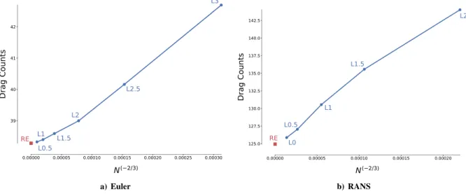
The baseline wing geometry for the Euler and RANS analyses is planar with a chord of 1.0 m and a NACA 0012 airfoil cross-section. The wingtip cap is a perfect revolution about the airfoil chord line and adds 0.06 m to the 3.0 m rectangular portion of the wing, bringing the total semispan to 3.06 m. The Euler geometry has a sharp trailing edge, while the RANS geometry has a blunt trailing edge with a thickness of 2.52 mm. We generate the surface meshes using Ansys ICEM CFD and employ pyHyp to create hyperbolically smoothed volume meshes. The meshes are oriented with the x-axis in the streamwise direction, the z-axis out the wing, and the y-axis in the vertical direction. The quality of these meshes is tested in a grid convergence study at the nominal baseline condition (M=0.5,Re=5×106_,

CL=0.2625), the results of which are plotted in Figure1. Table1lists the data for the baseline grids that are used in the optimization studies.

0.00000 0.00005 0.00010 0.00015 0.00020 0.00025 0.00030

N

Drag Counts

N

Drag Counts

Figure 1. Grid convergence study atM=0.5,Re=5×106_andC

L=0.2625. The zero-spacing grid, computed with Richardson extrapola-tion, is marked with RE for each set of grids.

We use a free-form deformation (FFD) volume method to manipulate the geometry. In this approach, the design variables are linked to the control points of a B-spline volume. The surface nodes of the mesh are embedded inside this B-spline volume and any displacements of the control points are interpolated to the surface mesh. These manip-ulations to the surface mesh are then propagated out to the volume mesh by way of an unstructured mesh-warping algorithm [18]. Our method allows the definition of global and local design variables. The global design variables act on a group of the FFD control points, facilitating large-scale deformations, while the local shape design variables

b_{https://github.com/mdolab/OpenAeroStruct}

Table 1. Baseline geometry performance atCCCLLL===000...222666222555

Grid Cells α CD(counts)

Euler L3 180,992 3.023 42.694

Euler L2 1,447,936 3.030 38.997

RANS L2 306,432 3.206 146.274

RANS L1 2,451,456 3.205 132.195

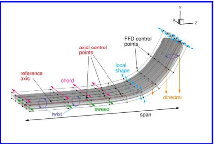
allow individual displacement of each control point. Figure2depicts the FFD volume, control points, and the design variables definitions for this case. The nominal FFD volume has nine spanwise control sections and 12 chordwise control points per section with half of the points on the upper surface and the other half on the lower surface. The global variables are linked to the displacement and rotation of axial control points along the reference axis. Each of these axial control points dictates the global movement of an entire FFD control section. The local shape variable definition requires some explanation. Each spanwise control section is assigned a unique reference frame with the section plane normal as the ˆek axis, the ˆei axis aligned with the streamwise direction, and ˆej=eˆk×eˆi. The local shape variables control the movement of the control points along their respective ˆej axes. When the reference axis is displaced vertically, the control sections and their respective reference frames are automatically rotated to remain perpendicular to it. This behavior is depicted in the formation of the winglet on the wing in Fig.2. The displacement vectors of the local shape variables in the wingtip control section are rotated as the winglet forms to allow sectional control of the airfoil section of the winglet. This functionality ensures that the wing surface does not shear, causing negative volumes, when large changes in dihedral are introduced.

In some cases, the large geometric deformations allowed in the present study cause negative volumes to form in the warped mesh. When this happens the optimizer is notified of the failure and usually it can backtrack and find a feasible point from which to continue the optimization. However, in some cases, the optimizer is unable to find a satisfactory point because the negative volumes occur in the region of the optimum. The remedy for this situation is to re-extrude the volume mesh from the deformed surface mesh. In many of the results presented herein, we use this approach to allow the optimizer to converge to the optimal wing shape.

Figure 2. Wing embedded in the FFD volume. The black dots represent the control points. The nominal FFD has nine sections of control points along the span of the wing, with tighter clustering toward the wingtip. Each section has six control point pairs along the chord. The shape variables are defined as the out-of-wing displacements of the control points within their respective control section planes. The global design variables are defined with respect to the axial control points, depicted with red cubes. The reference axis is shown at the quarter chord location, but in some cases it is placed along the trailing edge.

2.3. Low-fidelity Optimization: OpenAeroStruct

OpenAeroStruct [23] is an open-source low-fidelity aerostructural optimization suite developed using the OpenMDAO framework [24]. The aerodynamic analysis in OpenAeroStruct is performed using a vortex lattice method (VLM) to compute induced drag and a modified flat-plate skin-friction drag approximation to estimate viscous drag. These

fidelity models provide reasonable estimates at a low computational cost. A single analysis takes less than one second and a full optimization takes on the order of 10 seconds on a single processor. For the analyses in this study, the baseline geometry consists of a 1 m×3.06 m rectangular half-wing discretized by 50 spanwise panels and mirrored across the symmetry plane. The thickness-to-chord ratio and location of maximum thickness from the NACA 0012 airfoil are used in the computation of viscous drag. The geometry is parametrized using B-splines to interpolate variable changes to the geometry. Using B-splines allows a reduction in the number of design variables so that 50 panels can be manipulated with only 9 spanwise control points.

2.4. Optimizer

Both MACH and OpenAeroStruct are optimizer-independent, but for this study we use SNOPT [25] exclusively. SNOPT is a sequential quadratic programming, gradient-based optimizer which has been thoroughly vetted for aero-dynamic shape optimization and aerostructural design optimization [10–13].

2.5. Optimization Problem

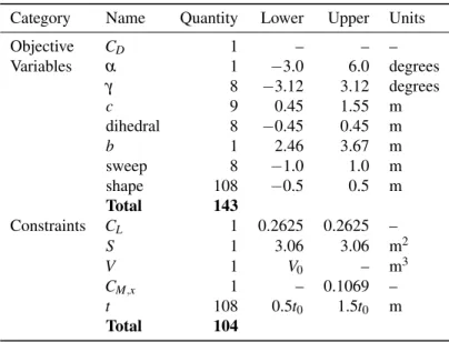
The complete optimization problem of ADODG Case 6 is defined in Table2. Twist variables are defined at every axial control point except at the root andα is used to match theCL constraint. The chord variables affect all nine axial control points. In the Euler cases, when local shape variables are inactive, the chord scales while maintaining constantt/c. Dihedral is defined as the vertical displacement of each axial control point. Additionally, the FFD section corresponding to each axial control point rotates to align the twist rotation and any shape variable displacements to be perpendicular to the wing surface. Sweep is defined as the streamwise displacement of each axial control point. Both dihedral and sweep are fixed at the root. As explained previously, the local shape variables perturb the wing cross-section perpendicular to the wing surface, such that they have some dependence on the dihedral variable. All control points in a given section are perturbed in a uniform direction, as indicated in Fig.2. The planform area,S, is computed as the area of the wing projected onto the x-z plane. Constraints for volume (V) and thickness (t) are handled by first setting up a 2D grid of points inside the surface of the wing. Then these points are projected to the surface of the wing to create a 3D grid confined within the wing. We computeV as the sum of the cell volumes andt

as the difference between the projected points on the upper and lower surface. The thickness constraints are evaluated at ten uniformly-spaced chord-wise locations ranging from 0.005cto 0.99cfor ten sections along the span. There are an additional eight thickness constraints added in the wingtip cap, making a total of 108 thickness constraints. The optimization cases treated in Section3 are subproblems of this full problem, and the variables and constraints are defined as stipulated in this full problem description unless otherwise stated.

Table 2. ADODG Case 6 Optimization Problem Statement

Category Name Quantity Lower Upper Units

Objective CD 1 – – – Variables α 1 −3.0 6.0 degrees γ 8 −3.12 3.12 degrees c 9 0.45 1.55 m dihedral 8 −0.45 0.45 m b 1 2.46 3.67 m sweep 8 −1.0 1.0 m shape 108 −0.5 0.5 m Total 143 Constraints CL 1 0.2625 0.2625 – S 1 3.06 3.06 m2 V 1 V0 – m3 CM,x 1 – 0.1069 – t 108 0.5t0 1.5t0 m Total 104

3.

Results

3.1. Twist Optimization

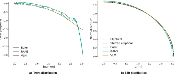
We begin with a simple twist optimization problem as a means of verification for our optimization framework. The twist optimization case has a long theoretical history and has also been extensively studied as a numerical optimization problem in ADODG Case 3 [26–28]. The elliptical twist distribution is well known as the theoretical optimum for this case because it generates the constant spanwise downwash required to minimize induced drag [29]. This theoretical result is a useful metric with which to gauge the performance of our optimization framework. Figure3 shows the optimal twist and lift distributions for the three levels of fidelity. We see very similar trends from each of the analyses, but there is a noticeable offset between the lift distributions from ADflow and the VLM results. This discrepancy is due to the rounded wingtip cap used for the Euler and RANS geometries. In the lifting-line model, the entire span is used to generate lift, whereas with the wingtip cap, the leading and trailing edges are truncated at 3 m of span and the last 0.06 m of span is incapable of generating the lift required to complete the elliptical distribution. As a result, the optimizer converges to a wing that generates an elliptical lift distribution extending from the root to the edge of the wingtip cap. Table3lists the drag counts of the optimized wings and the percent difference from the baseline drag value, %∆CD,base. As an added verification, we experimented with varying the number and spacing of the twist variables along the span and also started the optimization from ten random starting points. All of these variations yielded consistent results, which leads us to confirm the theoretical assertion that there is a single twist distribution that produces the lowest drag.

0.0 0.5 1.0 1.5 2.0 2.5 3.0

Span (m)

Twist (degrees)

Euler

RANS

VLM

z (m)

Normalized Lift

_Elliptical

Shifted elliptical

Euler

RANS

VLM

b) Lift distribution

Figure 3. In both Euler and RANS optimizations, the optimal twist distribution generates a lift distribution that matches the elliptical profile predicted by Prandtl’s classical lifting line theory. Due to the rounded wingtip cap that begins at 3.0 m, the lift distribution matches an elliptical distribution that extends from the root to the beginning of the cap. The RANS twist distribution appears discontinuous due to the twist angle being computed with reference to the top and bottom of the blunt trailing edge at different points along the span.

Table 3. Twist optimization results

Case Grid CL Drag counts %∆CD,base

Euler L3 0.2625 42.105 −1.38

RANS L2 0.2625 143.377 −1.98

VLM – 0.2625 128.779 −0.42

3.2. Chord Optimization

Different behaviors arise when drag is minimized by varying the chord distribution while keeping the twist constant. Theoretically, the elliptical chord distribution should be optimal for minimizing induced drag, and historically, this concept has been put to the test in the design of actual aircraft, most notably the Supermarine Spitfire. The optimization problem is to minimize drag with respect to the chord distribution, subject to the constraint thatCL=0.2625. Since the

lift coefficient is normalized byS, which may vary with changes in the chord, we must also constrainSto be constant. The inviscid and viscous results are henceforth discussed separately for each case to better explore and highlight the unique characteristics of each.

3.2.1. Euler

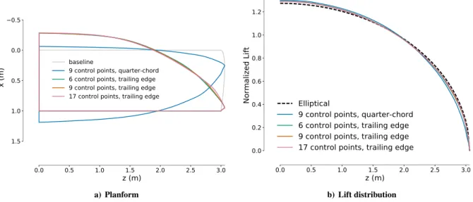
For the Euler chord optimizations we use the L3 mesh and change the bounds on the chord variables to (0.1, 2.0) to allow the planform to match an ellipse as close as possible. As in the twist optimization, the inviscid chord optimization yields predictable results. We take this predictability as an opportunity to test the sensitivity of the result to the chosen parameterization. We vary the number of spanwise FFD sections and corresponding chord variables and also compare the difference between scaling about the trailing edge and the quarter-chord. As shown in Fig.4, regardless of these modifications, each optimization converges to an elliptical lift distribution.

To test the multimodality of this problem, we started the optimization from ten random starting points. Nine of the starting points converged to the elliptical planform and one failed prematurely due to mesh warping errors. These results indicate that there is no multimodality in chord optimization for inviscid flow.

0.0 0.5 1.0 1.5 2.0 2.5 3.0

z (m)

x (m)

9 control points, quarter-chord 6 control points, trailing edge 9 control points, trailing edge 17 control points, trailing edge

a) Planform 0.0 0.5 1.0 1.5 2.0 2.5 3.0

z (m)

Normalized Lift

_Elliptical

9 control points, quarter-chord

6 control points, trailing edge

9 control points, trailing edge

17 control points, trailing edge

b) Lift distribution

Figure 4. Elliptical planform and lift distribution can be achieved by scaling the chord distribution about the quarter chord or the trailing edge. The effect of varying the number of FFD control sections is marginal.

Table 4. Chord optimization results

Case Grid CL Drag Counts %∆CD,base

Euler 1/4 chord L3 0.2625 41.726 −2.27

Euler 6 trailing edge L3 0.2625 40.439 −5.28 Euler 9 trailing edge L3 0.2625 40.412 −5.35 Euler 17 trailing edge L3 0.2625 40.356 −5.48

RANS L2 0.2625 142.544 −2.55 RANS mode 1 L1 0.2625 129.214 −2.26 RANS mode 2 L1 0.2625 129.178 −2.28 RANS monotonic L1 0.2625 129.296 −2.19 RANS L1 0.5 234.663 −1.23 RANS L1 0.8 503.049 −3.85 3.2.2. RANS

When adding viscous effects to the chord optimization, it is important to consider the trade-off between induced drag and viscous drag, and its relationship to chord length. While induced drag is sensitive to the spanwise distribution of

lift, viscous drag is highly dependent on the local chord length. The shear stress at the wall is directly related to the velocity gradient normal to the wall. For 2D laminar flow over a flat plate,

τw=µdu

dy (1)

This equation provides an approximation to the shear stress on an airfoil. At the leading edge, the boundary layer is very small and the velocity changes rapidly over a small distance, resulting in a large shear stress. Asx/cincreases, the boundary layer (BL) fills out and the velocity gradient at the wall becomes much more mild. The result is that extending the chord reduces the average drag per unit length. This relationship is well known and Blasius [30] provided the following analytic solution for the flat plate case,

cd=

1.328 √

Re, (2)

where the Reynolds number is based on the local chord. Multiplying by the local chord length we find that for constant flow conditions, the viscous drag per unit span is proportional to the square root of the local chord length, i.e.,

d∝

√

c (3)

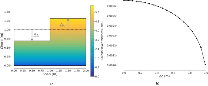
To illustrate this point, imagine we want to minimize the drag of a flat plate in laminar flow at zero angle of attack with a fixed planform area. If the chord distribution and span are variables, the chord distribution will grow to its upper limit and the span will adjust to satisfy the area constraint. However, if span is fixed, or has a hard lower limit, an interesting compromise takes place. The optimal chord distribution will have the maximum possible extent of the span at the upper limit of the chord variable. For example, if we split our plate into two independent sections and incrementally add∆cto the chord of one section while subtracting the same∆cfrom the other, we get a decrease in skin friction drag as shown in Figure5. In the absence of other constraints, lower skin friction drag can always be achieved by transplanting wing area from a thin-BL region to a thick-BL region. The spanwise location of the maximum chord region is irrelevant, and as such, a purely skin friction drag minimization problem theoretically has an infinite number of local minima.

0.00 0.25 0.50 0.75 1.00 1.25 1.50 1.75 2.00

Span (m)

Chord (m)

c

c

Boundar layer thickness (mm)

a) 0.0 0.2 0.4 0.6 0.8 1.0

c (m)

C

Figure 5. The viscous drag on a flat plate in laminar flow can be reduced by increasing the average BL thickness over the plate. In the left-hand plot, we reduce the chord on one half of the plate by∆∆∆cccwhile simultaneously increasing the chord on the other half to preserve the total planform area. The resulting decrease in viscous drag, as a function of∆∆∆cccis shown in the plot on the right. (Re=106)

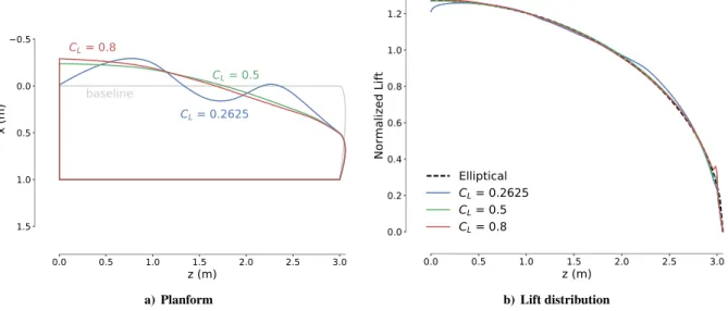
The problem becomes more complex when the objective function is a combination of both skin friction and induced drag. Minimum skin friction drag favors radical changes in the chord distribution to maximize thick-BL coverage, but optimal inviscid drag calls for an elliptically tapered wing. The optimal planform shape will balance these considera-tions taking into account the relative weights of each drag component. For instance, if drag is mostly induced (i.e., at highCL), the planform will take on a nearly elliptical profile. However, if we make some slight modifications to the planform, we may get some improvement in the viscous drag while not straying too far from the elliptical lift distribu-tion. This line of reasoning helps to explain the results we get from the RANS chord optimization, shown in Figure6.

These results are obtained using the RANS L1 mesh. For a givenCL, we can estimate the minimum possible contribu-tion of induced drag to the total drag using Prandtl’s induced drag approximacontribu-tionCD,i=CL/πAR. ForCL=0.2625, viscous drag makes up roughly 70% of the total drag, and the optimal planform shape is far from elliptical. AsCL increases and induced drag increases relative to viscous drag, the optimal design more closely approaches the elliptical planform. Interestingly, even for the low-CLcases, the lift distribution oscillates close to the elliptical profile.

0.0 0.5 1.0 1.5 2.0 2.5 3.0

z (m)

x (m)

baseline

C

= 0.2625

C

= 0.5

C

= 0.8

z (m)

Normalized Lift

Elliptical

C

= 0.2625

C

= 0.5

C

= 0.8

Figure 6. At lowCL, the planform develops a wavy profile to maximize the chord length and reduce viscous drag. AsCLincreases, the waves collapse to match the elliptical lift distribution more closely.

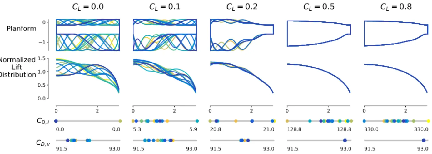
To address whether this trade-off between viscous and induced drag leads to multimodality at lowCL values, we first turn to a simpler aerodynamics model. Figure7shows the results of optimizing 20 random initial planforms at differentCL values with OpenAeroStruct. As expected, based on our previous discussion, the deviations from the elliptical lift distribution increase dramatically asCLdrops to zero. A corresponding decrease in viscous drag is small but noticeable. In the high-fidelity case we see similar trends. We optimize three randomly generated planforms at

CL=0.2625 with the RANS L1 mesh and the optimizer converges to two different planform modes. Wary of this result, we vary the number of control points used as design variables to rule out the possibility that our parametrization is biasing the results. We optimize the baseline geometry with 6 and 17 spanwise variables and compare the result with the baseline optimization with 9 spanwise variables. Despite the variance in flexibility allowed by the number of spanwise control points, the optimizer converges on a very similar, albeit not identical, planform shape in all three cases. These experiments suggest that there are a limited number of modes with which the optimizer can minimize viscous drag while still maintaining a sufficiently elliptical lift distribution so that the total drag decreases. The results for both of these tests are shown in Fig.8. Incidentally, we began the chord optimization tests with the RANS L2 mesh, but found a lack of multimodality in the lowCLcases. Since this did not agree with our hypothesis, we refined the mesh and found that the finer mesh yielded sharper spanwise curvature due to the refinement of the spanwise grid spacing. The difference in the optimized result due to the mesh refinement can be seen in Fig.9. We surmise that the coarseness of the L2 mesh causes an increase in drag when the optimizer attempts to create the large-amplitude spanwise variations seen in Fig.8and thus artificially limits the design space. However, it should be noted that the same physical phenomenon is apparent in both meshes, although its effect is dampened due to the coarseness of the mesh.

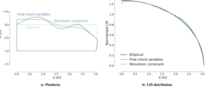
While these results are intriguing, we are ultimately interested to see how much of a benefit these spanwise os-cillations really provide. The VLM results suggest a drag decrease on the order of one to two counts. We add a monotonic constraint to the optimization of the L1 grid as a crude substitute for a more meaningful constraint, such as manufacturing cost and structural considerations. This constraint forces the chord distribution to decrease monotoni-cally from root to tip. The result is plotted in Figure9and detailed in Table4. Adding the monotonic constraint only increases the drag by a fraction of a drag count. This difference is not meaningful because it is within the modeling error. Furthermore, even if this difference were meaningful, it would be hard to justify the added manufacturing costs and structural penalties that would accompany building a wing with such spanwise curvature.

1 0

Planform

C

= 0.0

C

= 0.1

C

= 0.2

C

= 0.5

C

= 0.8

Normalized

Lift

Distribution

C

C

Figure 7. Twenty unique planform shapes are used to initialize an OpenAeroStruct chord optimization at 5 differentCLvalues. A trade-off exists between minimizing viscous drag by maximizing chord and forming an elliptic planform to minimize induced drag. AsCLincreases, induced drag makes up a greater portion of the total drag, and thus the planform approaches an elliptical shape and multimodality decreases. 0.0 0.5 1.0 1.5 2.0 2.5 3.0

z (m)

x (m)

Optimized planforms

Random initial planforms

a) Random starting points

0.0 0.5 1.0 1.5 2.0 2.5 3.0

z (m)

x (m)

Figure 8. (a) Starting the optimization from three random chord distributions reveals at least two local minima. These optimal planforms allow the chord to be maximized in some places while still generating a roughly elliptical lift distribution. (b) We experiment with varying the number of spanwise FFD sections and find that each parametrization yields a slightly different optimum when starting from the baseline. The general shape of the oscillating lift distribution remains the same.

0.0 0.5 1.0 1.5 2.0 2.5 3.0

z (m)

x (m)

baseline

Free chord variables

Monotonic constraint

z (m)

Normalized Lift

Elliptical

Free chord variables

Monotonic constraint

b) Lift distribution

Figure 9. Forcing the chord distribution to decrease monotonically from root to tip results in a more practical planform and sacrifices less than one count of the drag savings due to the spanwise oscillations.

3.3. Chord and Twist Optimization

Since we can reach an elliptical distribution with only chord design variables or only twist design variables, one may assume that a combination of both twist and chord variables would be redundant and lead to multimodality. We explore this possibility in this section.

3.3.1. Euler

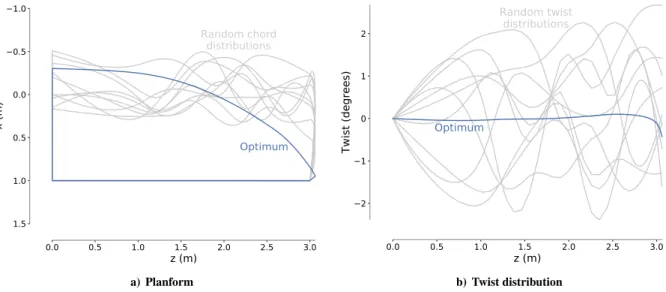
For the chord and twist optimization with Euler analysis we use the Euler L3 mesh and nine axial control points, corresponding to nine chord variables and eight twist variables. Once again, the limits on the chord variables are relaxed to 0.1≤c≥2.0 for the Euler cases. When initialized with ten different geometries, each generated with random chord and twist distributions, the optimizer converges to a single optimal solution. The optimal chord and twist distributions are superimposed over the randomly generated seeds in Fig.10. The uniformity of these results suggest that the chord and twist variables are not necessarily interchangeable. In Table5, we see that the addition of twist variables makes a negligible improvement in drag compared with the chord-only optimization (Table4).

3.3.2. RANS

The RANS optimizations are run using the RANS L1 mesh and the nominal 9-section FFD. The results are displayed in Figure11. We expect to see the oscillatory behavior observed at lowCLin the chord optimization to be exaggerated in this case because the twist can compensate for the deviations from the elliptical lift distribution that oscillations in the chord distribution would otherwise cause. The higherCLresults, like the Euler results, show little evidence of multimodality due to redundancy in the variables. ForCL=0.2625, the oscillations in the chord distribution are more prominent, which implies that the addition of twist variables grants more freedom to the chord variables to minimize viscous drag.

Table 5. Chord and twist optimization results

Case Grid CL Drag Counts %∆CD,base

Euler 1/4 chord L3 0.2625 41.517 −2.76

Euler L3 0.2625 40.408 −5.35

RANS L1 0.2625 128.802 −2.57

RANS L1 0.5 233.591 −1.68

RANS L1 0.8 480.496 −8.16

0.0 0.5 1.0 1.5 2.0 2.5 3.0

z (m)

x (m)

Random chord

distributions

Optimum

z (m)

Twist (degrees)

Random twist

distributions

Optimum

Figure 10. The wing optimization with respect to chord and twist variables using Euler analysis yields a single optimum when started from 10 random seeds. 0.0 0.5 1.0 1.5 2.0 2.5 3.0

z (m)

x (m)

baseline

C

= 0.2625

C

= 0.5

C

= 0.8

z (m)

Normalized Lift

Elliptical

C

= 0.2625

C

= 0.5

C

= 0.8

Figure 11. An optimization with both twist and chord variables tolerates more variation in the chord distribution at a lowerCL. AsCL increases, the planform shape oscillations disappear.

3.4. Dihedral and Twist Optimization

Nonplanar wings have the potential to reduce induced drag beyond what is attainable with a planar wing and an ellip-tical lift distribution. Previous optimization studies have verified this result [8,31]. We include twist variables in this subproblem because we want to allow the optimizer to converge to an elliptically loaded planar wing if that is the opti-mal design. However, we first assess the parametrization of the dihedral variables by conducting an optimization with just dihedral. Since we expect the most variation in dihedral to occur toward the wingtip, we want to make sure that our parametrization allows enough flexibility to capture the optimal shape. We vary the number of control points and ex-periment with spacing them uniformly along the span and clustering them more heavily toward the wingtip. In Fig.12 we compare the winglet-down optimized results for six different possible parametrizations. All six parametrizations achieved an elliptical lift distribution, but the cases with only six variables prevented the optimizer from converging to the optimal winglet cant angle. We chose to use the FFD with nine control points clustered toward the wingtip as the nominal FFD because it gives a sufficient degree of freedom to the optimizer for the kind of design space exploration we seek to do. Note that we recovered two local minima in the dihedral-only optimizations: an upturned winglet and a downturned winglet. The upturned winglet shapes were achieved when starting the optimization from random starting points; Figure12shows only the optima found when starting from the baseline geometry.

a) Front view 0.0 0.5 1.0 1.5 2.0 2.5 3.0

z (m)

Normalized Lift

Elliptical

6 linear

9 linear

17 linear

6 clustered

9 clustered

17 clustered

Figure 12. Comparison of different quantities and spanwise distributions of control points for an optimization with dihedral variables.

3.4.1. Euler

In the dihedral-only Euler case, there are two local minima: winglet-down and winglet-up wings. Here we combine twist and dihedral to see if the coupling between these two sets of variables affect the number of optima. We start the optimizations using the Euler L3 mesh (180k cells). Starting from 15 random variable sets the optimizer converges on more than two optima. Five of the optimizations converge to a winglet-up shape and the rest converge to a downturned winglet. Those that converge to the winglet-down shape share a very similar wingtip design, but vary in the vertical displacement of the main wing. These differences can be seen in Fig.13. To investigate the cause of these local minima, we take the uppermost (UWD) and lowest (LWD) optima in the winglet-down group and re-optimize them using the L2 mesh (1.45M cells). With the finer mesh, the optimizer converges to the same result for both of the coarse mesh local minima. Interestingly, this new result does not fall between the two starting seeds as we might expect. Instead, the optimizer pushes the wing down from the root to the midspan, at which point it slopes upward to merge with the downturned winglet of the coarse mesh results. When we start the optimization from the baseline rectangular wing with the L2 mesh, the optimizer converges on this same spoon-like shape. Re-optimizing the upturned winglet with the L2 mesh yields the same upturned winglet. We conclude that this case only has two physical optima and numerical noise causes additional optima when using the L3 mesh optimization results. When the mesh is coarse it loses resolution in critical areas, which leads to small changes in the objective function and creates more local minima. We extracted a design space slice between UWD and LWD for further analysis. Assume UWD and LWD have

design variable vectors X0 andX1. The set of all points on the line between UWD and LWD can be defined as

Xη=ηX0+ (1−η)X1, whereη∈[0,1]. We take 19 intermediary points along this line for the design space slice and computeCD at each point, taking care to adjustα to meet theCLconstraint. Figure14shows the slices inCDand

CL-space. Due to our settings of feasibility and optimality tolerance, the optimizer converged to UWD even though LWD has lower drag than UWD. The drag difference between UWD and LWD is on the order of 0.01 count, which is within the discretization error, and therefore not physically significant.

Figure 13. Euler dihedral and twist optimization results. Optimization with the L3 mesh (185k cells) produces an upturned winglet and a series of downturned winglets with variations in the midspan dihedral. We take the up optimum and the two outermost winglet-down optima (designated UWD and LWD) and re-optimize with the L2 mesh (1.45M cells). The winglet-up optima remains consistent, while both UWD and LWD converge to an entirely new spoon-like shape. When we run the L2 optimization from the baseline wing, the optimizer converges on the inverted spoon. The upturned winglet has lower drag than the downturned winglet for both the coarse and fine mesh optimizations.

Table 6. Dihedral and twist optimization results. TheCL=0.8result was obtained by regenerating the volume mesh to fix problems with the formation of negative volumes.

Case Grid CL Drag Counts %∆CD,base

Euler L3 0.2625 39.909 −6.52

RANS L2 0.2625 143.327 −2.01

RANS L2 0.5 244.969 −2.79

RANS L2 0.8 455.178 −15.91∗

3.4.2. RANS

The addition of viscosity to the model activates a trade-off between the induced drag improvement from winglet formation and the rise in viscous drag due to an increase in wetted area. Before running the RANS analyses, we explore the design space using OpenAeroStruct to better understand the implications of this trade-off. Figure 15 compares the optimization results for three general cases: inviscid analysis, viscous analysis, and viscous analysis

0.2 0.4 0.6 0.8 1.0 2 3 4 5 6 7 8 9 1e 11+2.624999999e 1

C

C

× 10

L3 mesh

L2 mesh

Figure 14. Design space slice with the L3 and L2 Euler meshes between two optima, UWD and LWD, showing the monotonic trend between them. Both coarse mesh optimizations converged optimality to the order of 1E-6, despite the decreasing slope between them. We surmise that numerical noise kept the optimizer from converging both results to the LWD point. It should be noted that these post-processed results matchedCLwithin a tolerance of10−9for each point, so theCDvalues for UWD and LWD are slightly different from their values in the optimization result.

with a monotonic constraint. The monotonic constraint forces the optimizer to form a downturned winglet, but the results are of interest because they give a metric with which to compare the unconstrained results. The three cases are optimized with 5 different starting points, displayed in the left-most column, and 5 different lift conditions ranging fromCL=0.1 toCL=0.8. The front views of each optimized wing profile are shown in each cell of the grid. Below and to the right of each wing profile, slider bars show the relative drag differences between the viscous-optimized results and the inviscid-optimized result. The horizontal bar shows the percent difference in inviscid drag, while the vertical bar indicates the percent difference in viscous drag compared with a viscous analysis of the inviscid-optimized result. Moving from the left to the right of the grid, the trend is an increase in nonplanarity for the viscous results. At lowCL values, when the viscous drag dominates, the optimizer has an incentive to reduce the arc length of the front view and thus reduce the effective wetted area. Since only small changes to the dihedral variables are possible without increasing the wetted area, the optimizer converges to the same optimum regardless of the starting point. As

CLincreases, this incentive diminishes and the optimizer tends toward more nonplanar wing shapes where the induced drag can be minimized. The increased freedom to vary the wing dihedral opens up the design space to multiple local minima. The inviscid optimization converges to three local minima and the viscous optimization forCL=0.8 converges to two optima: an upturned and a downturned winglet. The downturned winglet appears to offer better drag performance compared with the upturned winglet.

Taking the information from OpenAeroStruct as a reference, we optimize the RANS L2 baseline planform with respect to eight dihedral and twist variables forCL =0.2625, 0.5, and 0.8. The results once again demonstrate a strong dependence of the results onCL. As seen in left-hand side of Fig.16, the lowCL case deflects only slightly from the baseline geometry. AsCL increases, the vertical extent of the wing expands. Interestingly, when chord variables are added into the optimization, the trends seen in the separate chord and dihedral optimizations seem to be linearly combined with no recognizable coupling between dihedral and chord. This combined dihedral, twist, and chord optimization is presented on the right-hand side of Fig.16. In both of these cases, theCL=0.5 result converges to a down-turned winglet, while theCL=0.8 result converges to an upturned winglet. We run a dihedral and twist optimization for three wings with randomly distributed dihedral and twist atCL=0.5 to investigate the possibility of multiple local minima (Fig.17). Surprisingly, the optimizer converges to an upturned winglet for all three of these randomly generated wings, despite the fact that a comparison of drag values reveals a preference for the downturned winglet. We conclude that in an optimization where the parametrization allows for winglet formation, a gradient-based optimizer can converge to either an upturned or downturned winglet, depending on the starting position.

Inviscid optimum

Free planform

Monotonic constraint

% CD, v (compared to viscous analysis of inviscid optimum) -30.0 (better)

30.0 (worse) 0

-30.0 30.0

% CD, i

Initial

C

= 0.1

C

= 0.2

C

= 0.4

C

= 0.6

C

= 0.8

Figure 15. We use OpenAeroStruct to quickly explore the design space of the dihedral and twist optimization. The results in each column were constrained to the sameCL value and each row corresponds to the initial dihedral distribution in its left-most cell. The profiles in each cell represent the front profile of the half-wing. The key in the upper left corner provides labels for the different colors. Each optimization including viscous drag (blue or green) is compared with the same problem optimized with only inviscid drag (grey) by way of the accompanying horizontal and vertical bars. The horizontal bar indicates the percent difference in inviscid drag, while the vertical bar represents the percent difference in viscous drag. For this latter computation, the inviscid-optimized result was re-analyzed with consideration of viscosity. There are three local minima for the inviscid optimizations and two local minima for the high-CLviscous optimizations.

a) Dihedral and twist b) Dihedral, twist, and chord

Figure 16. (a) Adding dihedral to the RANS optimizations shows a preference toward a nonplanar wing asCLincreases. (b) When dihedral and chord variables are combined, we see a combination of the trends observed for each considered separately: the chord varies at lowCL and the winglet forms at a highCL.

Figure 17. Starting the dihedral and twist optimization from randomly generated starting points reveals two local minima, as expected. There is a slight preference towards the downturned winglet. These cases were constrained toCL=0.5.

3.5. Adding span and sweep variables

As a final step before considering the full case, we investigate the effects of adding span and sweep variables to the RANS optimization. Figure18shows the results of two distinct optimization problems. The left-hand side shows a comparison between optimizing with respect to twist, chord, dihedral, and span atCL=0.2625 andCL=0.5. The only geometric constraint is planform area. ForCL=0.2625, the optimizer finds greater benefit in maximizing the chord and does not increase span to reach the upper bound. The span does increase from the baseline case though, and the optimizer adds a slight anhedral to the wing. On the other hand, forCL=0.5, the span reaches the upper bound and an upturned winglet is formed.

When sweep is added to the optimization, we find the optimizer tends to sweep the wingtip back sharply, creating a raked wingtip. When the full bounds recommended in the ADODG case description are used, this sharply swept wing tends to cause mesh warping errors, resulting in negative volumes. To avoid this problem, we reduced the bounds to allow sweep to vary from−0.25 m to 0.25 m. The right-hand side of Fig.18shows the results of this optimization. The most noticeable feature of these results is the formation of the raked wingtip. Once again we notice that the optimizer does not extend to the full bounds of the span variable for the lower lift case. This time, forCL=0.5, the optimizer converges on a downturned winglet. When we run theCL=0.5 case starting from four random initial points with the L2 mesh, we find evidence of at least three local minima. Each of these local minima shares the distinct swept-back wingtip. The differences between them are due to the multimodality inherent to the other variables. One of the local minima has an upturned winglet while the others have a downturned winglet. Additionally, the chord distributions are unique between the local minima. The appearance of the same swept-back wingtip in all local minima, despite the differences in chord, dihedral, and sweep distribution on the main part of the wing, suggests that the sweep at the wingtip is highly beneficial to drag minimization.

a) Dihedral, twist, chord, and span b) Dihedral, twist, chord, span, and sweep

Figure 18. RANS optimization results starting from the baseline rectangular wing at differentCLvalues. The variables included in each case are listed.

3.6. Full Case Optimization

We now address the full ADODG case. All variables and constraints listed in Table2are included, except that sweep is limited to vary between−0.25 and 0.25 to avoid the negative volumes caused by extreme tip sweep.

3.6.1. Euler

Unfortunately, the results for the full Euler case are not as useful as we would hope. The full case includes a root bending moment constraint as a proxy for structural considerations, but the upper bound for this constraint does not allow the wing to support an elliptical lift distribution without decreasing the span. Rather than reduce the span to maintain the elliptical lift distribution the optimizer chooses to shift the lift distribution inboard, maintaining the span, but making the lift distribution less efficient. This results in a 300% increase in drag relative to the baseline mesh. From three random starting points, the optimizer converges on three separate local minima, all characterized by large spanwise oscillations in vertical displacement. From the lift distribution in Fig.19we can see that the outer wing is

generating negative lift to rein the root bending moment back beneath the upper limit of the constraint. To compensate for the negative outboard lift, the inboard section of the wing must produce even more lift to satisfy theCLconstraint, causing the increase in drag.

Since we are concerned with understanding the design space of the aerodynamic performance of the wing, we remove the root bending moment constraint to reduce the problem to pure aerodynamics. In total we found eight optima in the full case without the root bending moment constraint, and it is possible that there may be more local minima. We attempted five more optimizations, but these failed to converge to the desired tolerance. Figure20shows the eight successfully converged optima, which mainly form one winglet-up mode and one winglet-down mode. There is a great deal of variation in the spanwise chord distribution between the different optima. Most of the optima converge to a paddle-like shape with the maximum chord at the tip.

Figure 19. Results for the full ADODG Case 6 with Euler analysis atCL=0.2625. Negative lift is generated at the wingtip to satisfy the root bending moment constraint.

Figure 20. Removing the root bending moment constraint reveals the purely aerodynamics-based optimized result. These results are obtained with Euler analysis atCL=0.2625. Although some of the optimized shapes are similar, none of them converged to the same result.

3.6.2. RANS

Transitioning to RANS analysis, we again consider the full case with the root bending moment constraint included. AtCL=0.5, the stipulated upper bound of the bending moment constraint is too restrictive. To remedy this, we adjust the constraint such that the ratio ofCM,xin the baseline configuration to the value of theCM,xconstraint is the same for

CL=0.2625 andCL=0.5. This yields an upper bound ofCM,x=0.2046 for the root bending moment in the higher lift case (compared with 0.1069 atCL=0.2625). We run five optimizations for theCL=0.2625 condition and one optimization forCL=0.5. In Figure21, we show the two local minima found forCL=0.2625 and the single result for

CL=0.5. The effect of the root bending moment constraint on these optimizations is similar to the Euler results. The optimizer chooses to generate negative lift on the outboard section of the wing, as seen in the lift distribution plots. Notably, in the RANS optimizations the wing is tapered from root to tip, as opposed to the paddle-like planforms seen in the Euler results. In the low-CL results, we see the formation of an upturned and downturned winglet, as expected from our previous analysis of the dihedral variable. Additionally, the optimizer creates a swept-back wingtip for bothCLconditions. AsCLincreases, the wing shape starts to the develop the spanwise oscillations in the dihedral distribution that are produced in the Euler optimization.

a)CL=0.2625 b)CL=0.5

Figure 21. These are the results of the full ADODG case optimized with RANS analysis. For the lowCLcase, two local minima are found out of five cases run: one with dihedral and the other with anhedral. AtCL=0.5, the high-amplitude spanwise oscillations in vertical displacement seen in the Euler optimized results start to appear. In both cases, the outboard section of the wing generates negative lift to satisfy the root bending moment constraint.

Removing the root bending moment constraint facilitates a better understanding of the purely aerodynamic design space. We perform another round of RANS optimizations atCL=0.5 for the full case with no root bending moment constraint. Of four randomly-started optimizations, the optimizer recovers three local minima. The four results are shown in Figure22. The swept-back wingtip is common to all three local minima. Most of the variation between the local minima appears to be related to the multimodality inherent to the chord and dihedral variables which we discuss in detail in the respective subproblems. Where previously the chord tapered monotonically from root to tip forCL=0.5, we now see another mode of planform variation appear in two of the local minima. This new mode is characterized by a small root chord that expands into a large bulge at midspan and then tapers back down at the wingtip. The emergence of another planform mode indicates that the optimizer is granted more freedom in the chord variables because of the addition of other variables. A drag comparison between the two modes reveals that the midspan chord bulge is detrimental to the performance of the wing, resulting in a drag rise of approximately five counts. The variation in dihedral between the local minima reveals nothing new; two have an upturned winglet and the other has a downturned winglet. Of the two optima with the midspan chord bulge, the one with the downturned winglet generates significantly less drag, corroborating previous findings. The best-performing wing of the four results reduces the drag 22.5% from the baseline rectangular wing to 195.21 drag counts.

Due to the impractical bulge in the chord distribution found in two of the local minima for the RANS full case with no root bending moment, we run a similar case with the addition of a monotonic constraint on the chord distribution. Two results of this optimization problem are displayed in Figure22. The optimizer produces one upturned winglet and one downturned winglet. Once again, the downturned winglet outperforms the upturned winglet. The downturned winglet follows the same sweep trend seen in previous results, but the upturned winglet is swept forward at the wingtip, giving the first indication of a possible local minima in the sweep distribution. The drag performance of the monotonic downturned wing is better than any previous results, providing a 22% decrease relative to the baseline rectangular wing. This suggests that the addition of practical design constraints may actually help the optimization.

a) Full case with no root bending moment constraint b) Full case with a monotonic constraint on the chord distribution and no root bending moment constraint

Figure 22. RANS optimizations with no root bending moment constraint atCL=0.5. (a) Three local minima are found when starting the optimization from four random initial shapes. The multimodality appears to be mainly a function of the chord and dihedral variables. All results share the swept-back wingtip. (b) We add a monotonic constraint to the chord distribution to filter out impractical planform shapes. Each of the two cases run converges to a different result. The downturned winglet is characterized by the same forward swept main wing and backward swept wingtip seen in previous results. The upturned winglet is swept forward at the wingtip, which contradicts the observed trend and appears to increase drag by several counts.

4.

Conclusion

Wing aerodynamic optimization with respect to planform variables involves a strong trade-off between induced and viscous drag. The inclusion of a viscous drag model in the optimization is necessary to fully account for this trade-off and obtain physically meaningful results. In a chord optimization, at lowCLvalues, this trade-off causes the optimizer to form nonintuitive wavy chord distributions that minimize viscous drag at the cost of a perfectly elliptical lift distribution. This trade-off introduces multimodality into the design space, which we explained by analyzing a canonical flat plate with zero lift. In this extreme case, the optimal chord distribution is governed by the motivation to increase the chord as much as possible to reduce the skin friction drag per unit area while meeting the wing area constraint, but multiple chord distributions yield the minimum drag solution. AsCL increases, this multimodality is eliminated by the increasing relative importance of induced drag because the induced drag is also coupled with the chord distribution.

The benefit of nonplanarity is strongly correlated with the drag trade-off as well. When optimizing with respect to dihedral variables, the optimizer forms a winglet, for bothCL=0.5 andCL=0.8. The optimizer also displaces the main wing vertically in the opposite direction of the winglet to maximize the vertical extent of the wing and thus the vorticity sheet. This trend is amplified forCL=0.8 compared withCL=0.5. On the other hand, for a lowCL condition, the decrease in induced drag due to nonplanarity does not outweigh the increase in viscous drag due to the additional wetted area. Thus, for highCLconditions, dihedral variables add multimodality to the design space.

We find that a down-turned winglet reduces drag more than an upturned winglet, but both are local minima. A wing optimized with respect to both chord and dihedral variables appears to linearly combine the trends found in the separate cases: at lowCLthe planform is wavy with indiscernible dihedral, and at highCLthe wing tapers to a winglet. For each lift condition there is an optimal aspect ratio. When induced drag is the principal drag component, this optimal aspect ratio may not be possible due to span restrictions. However, we find that atCL=0.2625, the optimal aspect ratio is attainable within the bounds of the span variable, such that the optimizer does not extend the wing to the maximum possible span. Finally, when the optimizer has freedom to control sweep, it almost always converges to a wing with a sharply swept wingtip. Additionally, for the higher lift case, we see a tendency for the optimizer to sweep the wing forward slightly as if to amplify the effect of the swept-back wingtip.

We do find evidence of multimodality in the design space for both Euler and RANS analyses. In at least one case, the consideration of viscosity adds multimodality to the problem. However, in a problem with a highly flexible geometric parametrization, a comparison of Euler and RANS optimization results reveals the necessity of considering viscous effects. Although multimodality still exists with viscous analysis included, the results can be explained by the real physics, whereas with Euler analysis the explanation is not as readily apparent.

There are a few avenues for future work to build on these results. Since the optimal wing design is strongly dependent onCL, it would interesting to run an optimization considering multiple flight conditions. This would give a more realistic representation of real-world wing performance. Additionally, a structural model should be considered, since real-world wing design requires aerostructural analysis and design trade-offs.

5.

Acknowledgements

This research was partially funded by Embraer S.A. The authors would like to thank Gaetan Kenway and John Jasa for their development of the MACH and OpenAeroStruct frameworks, respectively.

References

[2] Martins, J. R. R. A. and Lambe, A. B., “Multidisciplinary Design Optimization: A Survey of Architectures,”AIAA Journal, Vol. 51, No. 9, September 2013, pp. 2049–2075.

[3] Chittick, I. R. and Martins, J. R. R. A., “An Asymmetric Suboptimization Approach to Aerostructural Optimization,” Opti-mization and Engineering, Vol. 10, No. 1, March 2009, pp. 133–152.

[4] Hicks, R. M. and Henne, P. A., “Wing Design by Numerical Optimization,”Journal of Aircraft, Vol. 15, No. 7, 1978, pp. 407– 412.

[5] Jameson, A., Pierce, N., and Martinelli, L., “Optimum aerodynamic design using the Navier-Stokes equations,” 35th Aerospace Sciences Meeting and Exhibit, Jan 1997.

[6] Ishimitsu, K., “Aerodynamic design and analysis of winglets,”Aircraft Systems and Technology Meeting, 1976, p. 940. [7] Pfeiffer, N., “Numerical winglet optimization,”42nd AIAA Aerospace Sciences Meeting and Exhibit, 2004, p. 213.

[8] Jansen, P. W., Perez, R. E., and Martins, J. R. R. A., “Aerostructural optimization of nonplanar lifting surfaces,”Journal of Aircraft, Vol. 47, No. 5, 2010, pp. 1490–1503.

[9] Martins, J. R. R. A., Alonso, J. J., and Reuther, J. J., “High-Fidelity Aerostructural Design Optimization of a Supersonic Business Jet,”Journal of Aircraft, Vol. 41, No. 3, May 2004, pp. 523–530.

[10] Lyu, Z., Kenway, G. K. W., and Martins, J. R. R. A., “Aerodynamic shape optimization investigations of the common research model wing benchmark,”AIAA Journal, Vol. 53, No. 4, 2014, pp. 968–985.

[11] Kenway, G. K. W. and Martins, J. R. R. A., “Multipoint High-Fidelity Aerostructural Optimization of a Transport Aircraft Configuration,”Journal of Aircraft, Vol. 51, No. 1, Jan 2014, pp. 144–160.

[12] Brooks, T. R., Kennedy, G. J., and Martins, J. R. R. A., “High-fidelity Multipoint Aerostructural Optimization of a High Aspect Ratio Tow-steered Composite Wing,” 58th AIAA/ASCE/AHS/ASC Structures, Structural Dynamics, and Materials Conference, 2017, p. 1350.

[13] Burdette, D. A., Kenway, G. K. W., and Martins, J. R. R. A., “Aerostructural design optimization of a continuous morphing trailing edge aircraft for improved mission performance,” 17th AIAA/ISSMO Multidisciplinary Analysis and Optimization Conference, 2016, p. 3209.

[14] Lyu, Z. and Martins, J. R. R. A., “Aerodynamic Design Optimization Studies of a Blended-Wing-Body Aircraft,”Journal of Aircraft, Vol. 51, No. 5, Sep 2014, pp. 1604–1617.

[15] Mader, C. A., Kenway, G. K. W., Martins, J. R. R. A., and Uranga, A., “Aerostructural Optimization of the D8 Wing with Varying Cruise Mach Numbers,”18th AIAA/ISSMO Multidisciplinary Analysis and Optimization Conference, Jun 2017.

[16] Gagnon, H. and Zingg, D. W., “Two-Level Free-Form Deformation for High-Fidelity Aerodynamic Shape Optimization,” 12th AIAA Aviation Technology, Integration, and Operations (ATIO) Conference and 14th AIAA/ISSMO Multidisciplinary Analysis and Optimization Conference, Sep 2012.

[17] Hicken, J. E. and Zingg, D. W., “Aerodynamic optimization algorithm with integrated geometry parameterization and mesh movement,”AIAA journal, Vol. 48, No. 2, 2010, pp. 400–413.

[18] Kenway, G. K. W., Kennedy, G. J., and Martins, J. R. R. A., “A CAD-free approach to high-fidelity aerostructural optimiza-tion,”13th AIAA/ISSMO multidisciplinary analysis optimization conference, 2010, p. 9231.

[19] Chernukhin, O. and Zingg, D. W., “Multimodality and global optimization in aerodynamic design,”AIAA journal, Vol. 51, No. 6, 2013, pp. 1342–1354.

[20] Lyu, Z., Kenway, G. K. W., Paige, C., and Martins, J. R. R. A., “Automatic Differentiation Adjoint of the Reynolds-Averaged Navier–Stokes Equations with a Turbulence Model,”21st AIAA Computational Fluid Dynamics Conference, San Diego, CA, Jul. 2013.

[21] Kenway, G. K. W., Secco, N., Martins, J. R. R. A., Mishra, A., and Duraisamy, K., “An Efficient Parallel Overset Method for Aerodynamic Shape Optimization,”Proceedings of the 58th AIAA/ASCE/AHS/ASC Structures, Structural Dynamics, and Materials Conference, AIAA SciTech Formum, Grapevine, TX, January 2017.

[22] Kenway, G. K. W., Kennedy, G. J., and Martins, J. R. R. A., “Scalable Parallel Approach for High-Fidelity Steady-State Aeroelastic Analysis and Adjoint Derivative Computations,”AIAA Journal, Vol. 52, No. 5, May 2014, pp. 935–951. [23] Jasa, J. P. and Hwang, J. T., “OpenAeroStruct: An open-source tool to perform aerostructural optimization,” 2017.

[24] Gray, J., Hearn, T., Moore, K., Hwang, J. T., Martins, J. R. R. A., and Ning, A., “Automatic Evaluation of Multidisciplinary Derivatives Using a Graph-Based Problem Formulation in OpenMDAO,”Proceedings of the 15th AIAA/ISSMO Multidisci-plinary Analysis and Optimization Conference, Atlanta, GA, June 2014.

[25] Gill, P. E., Murray, W., and Saunders, M. A., “An SQP algorithm for large-scale constrained optimization,” Society for Industrial and Applied Mathematics, Vol. 47, No. 1, 2005.

[26] Lee, C., Koo, D., Telidetzki, K., Buckley, H., Gagnon, H., and Zingg, D. W., “Aerodynamic Shape Optimization of Benchmark Problems Using Jetstream,”53rd AIAA Aerospace Sciences Meeting, 2015, p. 0262.

[27] Nadarajah, S., “Adjoint-Based Aerodynamic Optimization of Benchmark Problems,”53rd AIAA Aerospace Sciences Meeting, 2015, p. 1948.

[28] Poole, D. J., Allen, C. B., and Rendall, T., “Control Point-Based Aerodynamic Shape Optimization Applied to AIAA ADODG Test Cases,”53rd AIAA Aerospace Sciences Meeting, 2015, p. 1947.

[29] Munk, M. M., “The Minimum Induced Drag of Aerofoils,” 1923.

[30] Blasius, H., “Grenzschichten in Fl¨ussigkeiten mit kleiner Reibung,” Zeitschrift f¨ur angewandte Mathematik und Physik, Vol. 56, 1908, pp. 1–37.

[31] Khosravi, S. and Zingg, D. W., “Aerostructural Perspective on Winglets,”Journal of Aircraft, 2017.

This article has been cited by:

1. D. J. Poole, C. B. Allen, T. C. S. Rendall. Global Optimization of Wing Aerodynamic Optimization Case Exhibiting Multimodality. Journal of Aircraft, ahead of print1-16. [Abstract] [Full Text] [PDF] [PDF Plus]

2. John P. Jasa, John T. Hwang, Joaquim R. R. A. Martins. 2018. Open-source coupled aerostructural optimization using Python.

Structural and Multidisciplinary Optimization36. . [Crossref]

3. Yin Yu, Zhoujie Lyu, Zelu Xu, Joaquim R.R.A. Martins. 2018. On the Influence of Optimization Algorithm and Initial Design on Wing Aerodynamic Shape Optimization. Aerospace Science and Technology . [Crossref]