Syracuse University Syracuse University
SURFACE
SURFACE
Electrical Engineering and Computer Science College of Engineering and Computer Science
2003
Privacy-Preserving Collaborative Filtering Using Randomized
Privacy-Preserving Collaborative Filtering Using Randomized
Perturbation Techniques
Perturbation Techniques
Huseyin PolatSyracuse University Wenliang Du
Syracuse University, [email protected]
Follow this and additional works at: https://surface.syr.edu/eecs Part of the Computer Sciences Commons
Recommended Citation Recommended Citation
Polat, Huseyin and Du, Wenliang, "Privacy-Preserving Collaborative Filtering Using Randomized Perturbation Techniques" (2003). Electrical Engineering and Computer Science. 18.
https://surface.syr.edu/eecs/18
This Working Paper is brought to you for free and open access by the College of Engineering and Computer Science at SURFACE. It has been accepted for inclusion in Electrical Engineering and Computer Science by an authorized administrator of SURFACE. For more information, please contact [email protected].
Privacy-Preserving Collaborative Filtering using
Randomized Perturbation Techniques
Huseyin Polat and Wenliang Du Systems Assurance Institute
Department of Electrical Engineering and Computer Science Syracuse University, 121 Link Hall, Syracuse, NY 13244
Email: {hpolat,wedu}@ecs.syr.edu
Abstract
Collaborative Filtering (CF) techniques are becoming increasingly popular with the evolution of the Internet. E-commerce sites use CF systems to suggest products to customers based on like-minded customers’ preferences. People use CF systems to cope with information overload. To conduct collaborative filtering, data from customers are needed. However, collecting high quality data from customers is not an easy task because many customers are so concerned about their privacy that they might decide to give false information. CF systems using these data might produce inaccurate recommendations.
We propose a randomized perturbation technique to protect users’ privacy while still pro-ducing accurate recommendations. Although the randomized perturbation techniques add ran-domness to the original data to prevent the data collector from learning the private user data, our scheme can still provide recommendations with decent accuracy. We conducted several ex-periments to compare the recommendations on the randomized data with those on the original data. Using these experiment results, we analyzed how different parameters affect the accuracy. Our results show that the CF systems using the randomized perturbation techniques provide accurate recommendations while preserving the users’ privacy.
Keywords: Privacy, Collaborative Filtering, Randomized Perturbation.
1
Introduction
With the amount of the information available for individuals growing steadily, information overload has become a major problem for users. To make the information to serve users better, information filtering and recommendation schemes become more and more important. Collaborative filter-ing (CF) or social filterfilter-ing is a recent technique for such filterfilter-ing and recommendation purposes.
The term “collaborative filtering” was first coined by the designers of Tapestry [7], a mail filter-ing software developed in the early nineties for the intranet at the Xerox Palo Alto Research Center. With the number of users accessing the Internet growing, CF techniques are becoming increasingly popular as part of online shopping sites. These sites incorporate recommendation systems that suggest products to users based on products that like-minded users have ordered before, or indicate as interesting. Collaborative filtering has many important applications [4, 5] in e-commerce, direct recommendations, and search engines. Users can get recommendations about many of their daily activities, including restaurants, bars, movies, books, news, music CDs, interesting sights to see, and things to do in a city with the help of collaborative filtering.
The goal of CF [13] is to predict the preferences of one user, referred to as the active user, based on the preferences of a group of other users. For example, given the active user’s ratings for several movies and a database of other users’ ratings, the system predicts how the active user would rate unseen movies. The key idea is that the active user will prefer those items that like-minded users prefer, or that dissimilar users do not. The fundamental assumption [8] is that if users A and B
rate k items similarly, they share similar tastes, and hence will rate other items similarly.
1.1 Privacy-Preserving Collaborative Filtering Problem
Today’s CF systems have a number of disadvantages [4, 5]. The most important is that they are a serious threat to individual privacy. There is a great potential for individuals to share all kinds of information about places and things to do, see and buy, but the privacy risks are severe. Most online vendors collect buying information and preferences about their customers and make reasonable efforts to keep this data private. However, customer data is a valuable asset and it has been sold when some e-companies suffered bankruptcy.
The fragility of the digital marketplace has put many e-companies in bankruptcy [5]. The courts have supported the rights of liquidators to sell off data about their customers’ personal information as an asset. From Amazon.com’s policy “In the unlikely event that Amazon.com, Inc., or substantially all of its assets are acquired, customer information will of course be one of the transferred assets.” This policy is typical of many other companies and, in spite of Amazon’s language, the papers are filled with news of such “unlikely events” which lead to bankruptcies and transfer of customer information.
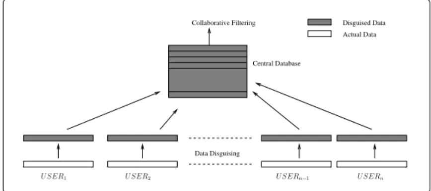
Disguised Data Actual Data Data Disguising Central Database Collaborative Filtering U SER2
U SER1 U SERn−1 U SERn
Figure 1: Privacy Preserving Collaborative Filtering
Some people might be willing to selectively divulge information if they can get benefit in re-turn [19]. Examples of the benefit provided include discount of purchase, useful recommendations, and information filtering. However, a significant number of people are not willing to divulge their information because of privacy concerns, according to a survey conducted in 1999 [6]. The challenge is how can users contribute their personal information for collaborative filtering purposes without compromising their privacy?
One way to achieve privacy is to use anonymous techniques [1, 14, 18], which allow users to disclose their personal information without disclosing their identities. The biggest problem of using anonymous techniques is that there is no guarantee on the quality of the dataset. A malicious user (e.g. a competing company) could send a great deal of random information to the database and render the database useless, or a company could send a lot of made-up information to the database with the goal of making their products the most favorable ones. These potential attacks could
database owner to control the quality of the data. It is important for the database owner to verify the identities of the data contributors in order to guarantee the quality.
Canny shows another way to conduct collaborative filtering without disclosing each user’s pri-vate data [4, 5]. The solution allows individuals both inside and outside the community to gain recommendations without learning each individual’s private data. In this scheme, many users need to participate in each recommendation.
1.2 Outline of Our Solution
We propose a new scheme in this paper to allow the privacy-preserving collaborative filtering. In our scheme (Fig. 1), each user first disguises his/her personal data, and then sends to a central place (the data collector), such that the data collector cannot derive the truthful information about a user’s private information. However, the data disguising scheme should still be able to allow the data collector to conduct collaborative filtering from the disguised data. We propose to useRandomized Perturbation techniques to disguise private data.
The basic idea of randomized perturbation is to perturb the data in such a way that the central place can only know the range of the data, and such range is broad enough to preserve users’ privacy. Although information from each individual user is scrambled, if the number of users is significantly large, the aggregate information of these users can be estimated with decent accuracy. Such property is useful for computations that are based on aggregate information. For those computations, we can still generate meaningful outcome without knowing the exact values of individual data items because the needed aggregate information can be estimated from the scrambled data. Since collaborative filtering is based on aggregate values of a dataset, rather than individual data items, we hypothesize that by combining the randomized perturbation techniques with collaborative filtering algorithms, we can achieve a decent degree of accuracy for the privacy-preserving collaborative filtering.
To verify this hypothesis, we implemented the randomized perturbation technique for a collab-orative filtering algorithm, which was proposed by [10]. We then conducted a series of experiments to show how accurate our results are. We compared the predictions that are calculated based on original data with the predictions on randomized data. Our results show that if the number of users and items are significantly large, the predictions we have found on randomized data are very close to the predictions found on the original data.
2
Related Work
2.1 Privacy-Preserving Collaborative Filtering
Canny proposes two schemes for privacy-preserving collaborative filtering [4, 5]. In these schemes, users control all of their own private data; a community of users can compute a public “aggre-gate” of their data without disclosing individual users’ data. The aggregate allows personalized recommendations to be computed by members of the community, or by outsiders. Canny’s method reduces the collaborative filtering task to an iterative calculation of the aggregate requiring only addition of vectors of user data. Canny then uses homomorphic encryption to allow sums of en-crypted vectors to be computed and deen-crypted without exposing individual data. His schemes are based on distributed computation of a certain aggregate of all users’ data. The aggregate is treated as public data. Each user constructs the aggregate and uses local computation to get personalized recommendations. Canny’s schemes can be implemented with untrusted servers, or with additional
infrastructures, as a fully peer-to-peer (P2P) system. The P2P architecture allows users to create and maintain their own recommender groups themselves.
While Canny’s work focuses on the peer-to-peer framework, in which users actively participate in the collaborative filtering process, our work focuses on another framework, in which users send their data to a central place and they do not participate in the CF process; only the central place needs to conduct the CF. Both frameworks have their applications. The peer-to-peer framework is more suitable in community-based CF systems while our framework is more suitable for systems that provide on-line CF services, such as Amazon, Yahoo travel, etc.
Randomized perturbation scheme was used by Agrawal and Srikant to solve privacy-preserving data mining problems [2]. The paper shows that it is possible to build decision tree classifiers if data is disguised using the randomized perturbation scheme. Our work solves a different but related problem.
2.2 Notations
We used the following notations in our study here:
vij is vote for userion item j.
wai is similarity weight between active user aand useri.
va is mean vote for active usera.
vi is mean vote for user i.
paq is prediction for active useraon item q.
σa is standard deviation of active usera’s ratings.
σi is standard deviation of useri’s ratings.
α is range of random numbers.
γ shows percentile of the data.
zij is z-score for user ion item j.
M AE is mean absolute error.
2.3 Collaborative Filtering Algorithms
There are two general classes of CF algorithms [3]. Memory-based algorithms operate over the entire user database to make predictions. Model-based CF algorithms use the user database to estimate or learn a model, which is then used for predictions. Cluster models and Bayesian network model are two of the model-based collaborative filtering algorithms. There is another classes of CF algorithms that are hybrid memory and model based algorithms [13].
The task in CF is to predict the votes of a particular user (the active user) based on a database of user votes from a sample or population of other users (the user database) [3]. The user database consists of a set of votes vij corresponding to the vote for useri on item j. The user database is
usually a sparse matrix. The users do not rate all of the items. The missing ratings can be filled by using the item mean vote, the user mean vote, or the overall mean vote [5].
In memory-based collaborative filtering algorithms, we predict the votes of the active user (indicated with a subscripta) based on some partial information regarding the active user and a set of weights calculated from the user database [3].
Memory-based algorithms can be divided into different sub-categories in terms of the details of the weight calculation. Pearson correlation coefficient and vector similarity are two of the methods of weight calculation.
Pearson Correlation Coefficient This formulation first appeared in the published literature in the context of the GroupLens project [15], where the Pearson correlation coefficient was defined as the basis for the weight calculation. The correlation between active useraand user iis [3]:
wai = X k (vak−va)(vik−vi) X k (vak−va)2 X k (vik−vi)2 1/2 (1)
where the summations over k are over the items for which both the active user a and the user i
have voted. va and vi are mean votes for active user aand user i, respectively. If Ii is the set of items on which user ihas voted, then we can define the mean vote for userias [3]:
vi= 1 |Ii| X j∈Ii vij (2)
Vector Similarity In vector similarity, each user votes are represented as a vector. The weights can be calculated as [3]: wai = X k vak X s∈Ia (vas)2 1/2 vik X s∈Ii (vis)2 1/2 (3)
whereIais the set of items on which active user ahas voted.
GroupLens introduced an automated collaborative filtering system using a neighborhood-based algorithm [12, 15]. GroupLens provided personalized predictions for Usenet news articles. The original GroupLens system used Pearson correlations to weight user similarity, used all available correlated neighbors, and computed a final prediction by performing a weighted average of devia-tions from the neighbor’s mean:
paq =va+ n X i=1 (viq−vi)·wai n X i=1 wai (4)
paq represents the prediction for the active user a on item q. n is the number of neighbors and
wai is the similarity weight between the active user a and the user i as defined by the Pearson correlation coefficient.
An extension of the GroupLens algorithm, which we use in our study in here was proposed by [10]. Herlocker et al. compare the performance of different normalization techniques such as the bias-from-mean, the z-scores, and the non-normalized rating. The z-scores perform significantly better than the non-normalized rating approach. The mean and the standard deviation of the z-scores are 0 and 1, respectively. If the vij is user i’s vote on item j, vi is the mean vote of the
user i, and σi is the standard deviation for the user i, then the z-scores (zij) can be defined as:
zij =
(vij−vi)
σi
Herlocker et al. [10] account for the differences in spread between users’ rating distributions by converting ratings to z-scores, and compute a weighted average of the z-scores:
paq =va+σa· n X i=1 (viq−vi) σi ·wai n X i=1 wai wai = X k (vak −va)·(vik−vi) σa·σi (6)
where k is the item set both the active user a and the user i have rated. σa and σi are standard deviations of the active usera’s ratings and the useri’s ratings, respectively.
There are also other memory-based collaborative filtering algorithms. The Ringo Music Rec-ommender [17] and the Bellcore Video RecRec-ommender [11] expanded upon the original GroupLens algorithm. Ringo used 4 as the mean vote for all users and limited membership when computing the weights while Bellcore Video Recommender selected the best neighbors to create a prediction. A constant time collaborative filtering algorithm was proposed by [8], which is based on principal component analysis (PCA).
3
Privacy Preserving CF using Randomized Perturbation
3.1 Randomized Perturbation TechniquesThere are several ways to hide numbers or information. To hide a numbera, a simple way is to add a random numberrto it. Although we cannot do anything toasince it is disguised, we can conduct certain computations if we are interested in the aggregate data, rather than each individual data.
The basic idea of randomized perturbation is to perturb the data in such a way that certain computations can be done while preserving users’ privacy. Although information from each indi-vidual user is scrambled, if the number of users is significantly large, the aggregate information of these users can be estimated with decent accuracy. Such property is useful for computations that are based on aggregate information. Scalar product and sum are among such computations and used in collaborative filtering algorithms. For those computations, we can still generate meaningful outcome without knowing the exact values of individual data items because the needed aggregate information can be estimated from the scrambled data.
Scalar Product LetAandBbe the original vectors, whereA= (a1, . . . , an) andB = (b1, . . . , bn).
A is disguised by R = (r1, . . . , rn), andB is disguised by V = (v1, . . . , vn), whereri’s andvi’s are
uniformly distributed in domain [−α, α]. Let A0
=A+R and B0
=B+V be the disguised data that are known, we now show how the scalar product of A and B can be estimated from A0 and B0 : A0 ·B0 = n X i=1 (aibi+aivi+ribi+rivi) BecauseR andB are independent, we have Pn
i=1ribi≈0; similarly we have Pn i=1aivi ≈0, and Pn i=1rivi ≈0. Therefore, we have n X i=1 (ai+ri)(bi+vi) = n X i=1 (aibi+aivi+ribi+rivi)≈ n X i=1 aibi (7)
Sum Let A be the original vector with n values, where A = (a1, . . . , an). A is disguised by
R = (r1, . . . , rn), where ri’s are uniformly distributed in domain [−α, α]. Let A0 = A+R be
the disguised data that is known. Since ri’s are uniformly distributed in domain [−α, α], the contribution of the sum of the random values to the actual sum of the values of vector A is close to zero. In the long run, the relative error will converge to zero. Therefore, we have
n X i=1 (ai+ri) = n X i=1 ai+ n X i=1 ri≈ n X i=1 ai (8)
Next, we will show how we use these two approximation techniques to conduct privacy-preserving collaborative filtering.
3.2 CF with Privacy using Randomized Perturbation Techniques
Our goal of collaborative filtering using randomized perturbation is to achieve privacy and pro-duce recommendations with high accuracy. However, achieving privacy and producing accurate recommendations are two conflicting goals. Users might send false data instead of their actual data to achieve perfect privacy. But producing accurate recommendations is impossible from this false data. On the other hand, if users send their actual data to the server, finding high quality recommendations is possible but the users’ privacy is not preserved. We propose a technique to achieve a good balance between the privacy and the accuracy.
Without privacy concerns, every user sends his/her ratings to the server, which creates a central database containing ratings from all users. To get a recommendation, an active user sends his/her known ratings and a query (for which item he/she is looking for prediction) to the server, and the server can calculate the paq (predicted vote for active useraon item q) using the Eq. (6).
With the privacy concerns, the server should not know the true data of each user including the active users. We use the randomized perturbation technique to achieve data disguise. In our approach, users add a random number to each of their actual ratings that they want to disguise, and send the results to the server. The server should not be able to find the true values of the ratings because of the random numbers. To show how our approach works, we use the z-score notation to simplify the Eq. (6):
ziq = viq−vi
σi (9)
Therefore, from Eq. (6) we get:
paq =va+σa·p 0 aq =va+σa· n X i=1 wai·ziq n X i=1 wai , wai= X k zak·zik (10) where p0aq = n X i=1 " X k zak·zik # ·ziq n X i=1 X k zak·zik = X k zak· " n X i=1 zik·ziq # X k zak· " n X i=1 zik # (11)
Since the active user and the other users have not rated all items, the counter, k, is different from user to user. Only those items that have been rated by both the active usera and the useri
are involved in computations. The entries for those items that have not been rated are zero. Notice that the nominator part consists of a scalar product between vector Zk= (z1k, . . . , znk)
and vector Zq= (z1q, . . . , znq). If the server can compute the scalar products for allk’s, it can send
the results of the scalar products to the active user who can easily compute the nominator part. The denominator part is even simpler. All the server needs to do is to send the result of Pn
i=1zik
for each k to the active user.
Based on the above observations, we develop the following scheme, such that each user does not need to send the actual information to the server while still allowing the server and the future active users to computep0aq jointly.
1. The server decides on a range [−α, α], and let each user know. How the server decides on the value of α will be discussed later.
2. Each usericomputes his/her mean vote, standard deviation, and then calculates the z-scores
zij for the items that he/she has rated.
3. Each user i creates ni uniform random numbers rij in the range [−α, α], where ni is the total number of items that user has rated; note that ni might be different from user to user
because every user might have rated different number of items. Userithen adds those random numbers to its z-score ratings and generates the disguised z-scores z0
ij =zij+rij. Userithen
sends the results (ni disguised z-scores) to the server.
After getting all the disguised z-scores z0
ij from many users, the server can now provide
collab-orative filtering services to active users based on the following facts from Eq. (7) and (8):
n X i=1 zik·ziq ≈ n X i=1 z0 ik·z 0 iq n X i=1 zik ≈ n X i=1 z0 ik (12)
To get a recommendation for item q, the active user computes the z-scores zak for those items
that he/she has rated before. Then, the server sends the results of
n X i=1 z0 ik·z 0 iq and n X i=1 z0 ik for all k
to the active user who uses Eq. (11) and (12) to compute p0
aq andpaq, the predicted rating for the
active useraon item q.
3.3 Selecting the Range of the Random Numbers
To protect the private data, the range of the random numbers is critical. If the range is too small, the perturbed data still discloses significant amount of information; if the range is too large, we hypothesize that the accuracy of the results will be very low. To understand how the range affects the accuracy, we associate the range with the distribution of the original data.
Let X = (x1, . . . , xn) be a vector, wherexi ∈[c, d] fori= 1. . . n. To disguise the values of the vector X using the randomized perturbation technique, we generate n uniform random numbers from [−α, α] and add them to the values of the vector X.
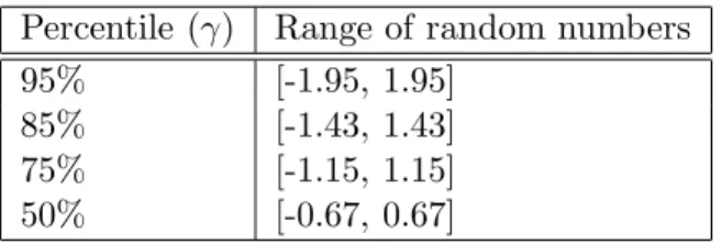
Percentile (γ) Range of random numbers 95% [-1.95, 1.95] 85% [-1.43, 1.43] 75% [-1.15, 1.15] 50% [-0.67, 0.67] Table 1: Examples
Assume the distribution (probability density function) of the random variablexfor the sequence inX isf(x). We calculate the percentile of the distribution, and find the range for this percentile. For example, for 95 percentile, we find a range inf(x), such that 95% of the data of this distribution falls into the range.
When the distribution is standard normal distribution, i.e. the distribution is a normal distri-bution with the mean (µ) being 0 and the standard deviation (σ) being 1, the ranges for certain percentiles can be looked up from a table. Fig. 2 shows the meaning of various percentiles for the standard normal distribution, and Table 1 shows the ranges of the random numbers for various percentiles in standard normal distribution.
−3 −2 −1 0 1 2 3 0 0.05 0.1 0.15 0.2 0.25 0.3 0.35 0.4 50% of the Data 75% of the Data 85% of the Data 95% of the Data
Figure 2: Standard Normal Distribution (mean 0, standard deviation 1)
From now on, we use γ to represent the percentile. After deciding the γ values, we can decide the range of the random numbers based on the distribution of the data.
3.4 Various Ways for Data Disguising
There are several ways we can disguise the original data using the random perturbation techniques.
• Fixed Range: We use a fixed range to generate random numbers. After deciding on the range of the random numbers, we generate random numbers uniformly within this range.
• Random Range: In this scheme, after deciding on the range of the random numbers, each user randomly generates a numberα within this range, and then uses [−α, α] as the range to generate uniform random numbers to disguise all his/her private data.
4
Experimental Results
4.1 DatasetsWe use Jester and MovieLens datasets in our experiments to evaluate the accuracy of our randomized-perturbation-based collaborative filtering scheme. We compare the predictions based on original data with the predictions calculated from randomized data using our scheme. We describe the details of the datasets in the following:
• Jester is a web-based joke recommendation system, developed at University of California, Berkeley [9]. The database has 100 jokes and records of 17,988 users. The ratings range from -10 to +10, and the scale is continuous. Some users end up reading and rating all the jokes, so Jester is much more dense than the other datasets we used. Almost 50% of all possible ratings are present.
• MovieLens data were collected by the GroupLens Research Project at the University of Min-nesota (www.cs.umn.edu/research/Grouplens). There are two datasets available. The first one (called MovieLens Public Data) consists of 100,000 ratings for 1,682 movies by 943 users. The second one (called MovieLens Million Data) consists of approximately 1 million ratings for approximately 3,500 movies made by 7,463 users. Each user has rated at least 20 movies. Ratings are made on a 5-star scale.
4.2 Evaluation Criteria
Several evaluation criteria for collaborative filtering have been used in literature [5, 10, 17]. The most common criteria are the Mean Absolute Error (MAE) and the standard deviation (σ). We also use these two criteria in our evaluation.
If p1, p2, . . . , pd are predicted values from undisguised data, and p01, p02, . . . , p0d are predicted values from disguised data, then E = {ξ1, ξ2, . . . , ξd} = {p
0 1 −p1, p 0 2 −p2, . . . , p 0 d−pd} represents
errors. Therefore, the MAE and the standard deviation of the errors are computed using the following equations: E= Pd i=1|ξi| d and σ= s Pd i=1(E−E)2 d−1 4.3 Methodology
The outline of our procedure is described in the following:
1. Selecting training and testing datasets. The MovieLens public dataset contains 943 users and 1,682 items. We randomly divided the dataset into a training set (900 users) and a testing set (43 users). For the Jester dataset, we randomly selected 5,000 users from the dataset for training data and 500 users for testing data; for the MovieLens million dataset, we randomly selected 3,000 users for training and 300 users for testing.
2. Prediction for active users. For each active user selected randomly from the testing dataset, we randomly select an item and use our randomized-perturbation-based scheme and the original algorithm, respectively, to predict the ratings on this item for this active user. We then calculate the difference of these two ratings. We run this prediction procedure for 100 times and calculate the mean absolute error and standard deviation of the errors.
We hypothesize that the privacy and accuracy depend on several factors including the selection ofα, theγ values that affect the range of the random numbers (α), the total number of users, and the total number of items. Therefore, we conducted the following experiments:
• Fixed α vs. Random α. We experimented with two different strategies regarding the range of the random numbers (which is used to disguise users’ private data): one requires users to select the random numbers from a fixed range [−β, β], where β is a constant number; the other strategy requires users to select the random numbers from a changing range [−α, α], whereα is a random number ranging from [0, β].
• Dense Datasets vs. Sparse Datasets: We conducted experiments on both dense and sparse datasets. Although Jester and MovieLens are sparse datasets, we converted them into dense datasets. There are different methods to deal with missing ratings including using the user mean, the item mean, or the overall mean vote [5]. We used the item mean votes [16] to convert sparse training datasets into dense datasets.
• The Selection of γ. The value ofγ decides the range of the random numbers. It is critical to the performance of our scheme. We conducted experiments for variousγ values, including 95%, 85%, 75%, and 50%, but we only showed the results whenγ is 95% and 50%.
• Sets of Experiments: We hypothesize that the randomized perturbation techniques give more accurate results when the number of users and/or items increases. To test this hypothesis, we conducted three sets of experiments: for the first and the second sets, we try to keep the number of users the same while changing the number of items; for the second and the third sets, we try to keep the number of items the same while changing the number of users. Since the third set needs to involve a large number of users, we conduct the third set of experiments on dense datasets (we need to convert the sparse training datasets into dense sets using the item mean votes).
4.4 Experimental Results
To evaluate our proposed schemes, we have conducted several experiments; we then compared the prediction results from randomized data (using our schemes) with the results from the original data. Fig. 3, Fig. 4, and Fig. 5 depict our results on three different datasets.
For both MovieLens datasets (MovieLens public data and MovieLens million data), when we chooseγ = 95% and the fixed-α scheme, the mean absolute error in our experiments is below 0.29. Since the rating range is from 1 to 5,M AE= 0.29 indicates our results are very close to the results generated from the original data. As we can see from both Fig. 3 and Fig. 4, the results get much better when we use the random-α scheme to generate the random numbers; the results also get better when we choose a smallerγ value, or increase the value ofn(the total number of users) and
t(the total number of items). We will discuss the effects of those changes later.
For the Jester dataset, when we choose γ = 95% and the fixed-α scheme, the mean absolute error in our experiments can reach as high as 1.4. However, in Jester dataset, the rating scale is from -10 to 10; an error of 1.4 is equivalent to 0.28 in a 1–5 scale. Therefore, the results for Jester dataset is similar to those from the MovieLens datasets.
We now show how the α selection scheme, the value of γ, and the value of n and t affect the accuracy of the results.
• Value ofnandt: Results on all three datasets show that the accuracy is improved when either of the following increases: the total number of users (n) or the total number of items (t)
1 2 3 0 0.05 0.1 0.15 0.2 0.25 Groups of Experiments
Mean Absolute Errors
γ=50%, randomly selected α γ=95%, randomly selected α γ=50%, fixed α γ=95%, fixed α First Group n=271 t=39 Second Group n=285 t=131 Third Group n=500 t=129
(a) The Mean Absolute Errors (rating range: 1–5) 1 2 3 0 0.05 0.1 0.15 0.2 0.25 Groups of Experiments
Standard Deviations of Absolute Errors
γ=50%, randomly selected α γ=95%, randomly selected α γ=50%, fixed α γ=95%, fixed α Frist Group n=271 t=39 Second Group n=285 t=131 Third Group n=500 t=129
(b) Standard Deviations of the Absolute Errors
Figure 3: MovieLens Public Dataset
1 2 3 0 0.05 0.1 0.15 0.2 0.25 Groups of Experiments
Mean Absolute Errors
γ=50%, randomly selected α γ=95%, randomly selected α γ=50%, fixed α γ=95%, fixed α First Group n=154 t=154 Second Group n=143 t=265 Third Group n=1000 t=261
(a) The Mean Absolute Errors (rating range: 1–5) 1 2 3 0 0.02 0.04 0.06 0.08 0.1 0.12 0.14 0.16 Groups of Experiments
Standard Deviations of Absolute Errors
γ=50%, randomly selected α γ=95%, randomly selected α γ=50%, fixed α γ=95%, fixed α First Group n=154 t=154 Second Group n=143 t=265 Third Group n=1000 t=261
(b) Standard Deviations of the Absolute Errors
1 2 3 0 0.25 0.5 0.75 1 1.25 1.5 Groups of Experiments
Mean Absolute Errors
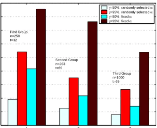
γ=50%, randomly selected α γ=95%, randomly selected α γ=50%, fixed α γ=95%, fixed α First Group n=250 t=32 Second Group n=263 t=69 Third Group n=1000 t=69
(a) The Mean Absolute Errors (rating range: -10–10) 1 2 3 0 0.1 0.2 0.3 0.4 0.5 0.6 0.7 0.8 0.9 Groups of Experiments
Standard Deviations of Absolute Errors
γ=50%, randomly selected α γ=95%, randomly selected α γ=50%, fixed α γ=95%, fixed α First Group n=250 t=32 Second Group n=263 t=69 Third Group n=1000 t=69
(b) Standard Deviations of the Absolute Errors
Figure 5: Jester Dataset
involved in the prediction calculation. The improvement trend can be observed from the differences of Group 1, 2, and 3. The reason of the improvement can be quite straightforwardly explained: Our scheme is based on the fact that the sum and the scalar product of the perturbed data are approximately the same as those of the original data. As we know, the more data we have for these two computations, the more accurate the approximation will be. In our scheme, increasingn and tis equivalent to increasing the amount of data involved in the sum and the scalar product computations.
• Selection of γ Value: Our results clearly show that the range of the random numbers affects the accuracy of our scheme. For example, in all of our result figures, results forγ = 50% are always better than those for γ = 95%. The range of random numbers is [-0.67, 0.67] when
γ = 50%, whereas it is [-1.95, 1.95] whenγ = 95%. As we know, when the range is small, the randomness also becomes smaller; thus the accuracy can be improved.
• Fixedαvs. Randomα: Our results show that the random-αscheme yields better performance than the fixed-α scheme. For example, in Fig. 3, whenγ = 95%, the error for the random-α
scheme is almost half of the error for the fixed-α scheme. The reason for this phenomenon is that when the range of the random numbers is random from [0, β], the distribution of all the random numbers is not uniform in range [−β, β]; the probability of choosing a number near 0 is larger than the probability of choosing a number nearβ or−β. On the other hand, in the fixed-α scheme, the generated random numbers are uniformly distributed in range [−β, β]. As we have already discussed, the bigger the random number, the less accurate the result. Therefore, choosing randomly selectedαas the range for the random numbers produces better results than the fixed-α scheme.
5
Conclusion and Future Work
We have presented a solution to the privacy-preserving collaborative filtering problem using the randomized perturbation scheme. Our solution makes it possible for servers to collect private data from users for collaborative filtering purposes without compromising users’ privacy requirements.
Our experiments have shown that our solution can achieve accurate prediction compared to the prediction based on the original data.
We believe that accuracy of our scheme can be further improved if more aggregate information is disclosed along with the disguised data, especially those aggregate information whose disclosure does not compromise much of users’ privacy. These types of information include mean, standard deviation, distribution, true data in a permuted order, etc. We will study how these kinds of aggregate data disclosure affects the accuracy and the privacy.
We will also study other collaborative filtering algorithms, and investigate whether we can extend our techniques to other memory-based and model-based algorithms to achieve privacy-preserving collaborative filtering.
References
[1] Anonymizer.com: http://www.anonymizer.com.
[2] R. Agrawal and R. Srikant. Privacy-preserving data mining. InProceedings of the 2000 ACM SIGMOD
on Management of Data, pages 439–450, Dallas, TX USA, May 15 - 18 2000.
[3] J. Breese, D. Heckerman, and C. Kadie. Empirical analysis of predictive algorithms for collaborative
filtering. In Proceedings of the Fourteenth Conference on Uncertainty in Artificial Intelligence, pages
43–52, Madison,WI, July 1998.
[4] J. Canny. Collaborative filtering with privacy. InIEEE Symposium on Security and Privacy, pages
45–57, Oakland, CA, May 2002.
[5] J. Canny. Collaborative filtering with privacy via factor analysis. In Proceedings of the 25th annual
international ACM SIGIR conference on Research and development in information retrieval, pages 238–245, Tampere, Finland, August 2002.
[6] L. F. Cranor, J. Reagle, and M. S. Ackerman. Beyond concern: Understanding net users’
atti-tudes about online privacy. Technical report, AT&T Labs-Research, April 1999. Available from
http://www.research.att.com/library/trs/TRs/99/99.4.3/report.htm.
[7] D. Goldberg, D. Nichols, B. M. Oki, and D. Terry. Using collaborative filtering to weave an information tapestry. 35(12):61–70, 1992.
[8] K. Goldberg, T. Roeder, D. Gupta, and C. Perkins. Eigentaste: A constant time collaborative filtering
algorithm. Information Retrieval, 4(2):133–151, 2001.
[9] D. Gupta, M. Digiovanni, H. Narita, and K. Goldberg. Jester 2.0: A new linear-time collaborative
filtering algorithm applied to jokes. InWorkshop on Recommender Systems Algorithms and Evaluation,
22nd International Conference on Research and Development in Information Retrieval, Berkeley, CA. [10] J. Herlocker, J. Konstan, A. Borchers, and J. Riedl. An algorithmic framework for performing
collab-orative filtering. InProceedings of the 1999 Conference on Research and Development in Information
Retrieval, August 1999.
[11] W. Hill, L. Stead, M. Rosenstein, and G. Furnas. Recommending and evaluating choices in a virtual
community of use. InProceedings of ACM CHI’95 Conference on Human Factors in Computing Systems,
pages 194–201, 1995.
[12] Joseph A. Konstan, Bradley N. Miller, David Maltz, Jonathan L. Herlocker, Lee R. Gordon, and John
Riedl. Grouplens: Applying collaborative filtering to usenet news. In Communications of the ACM,
pages 77–87, March 1997.
[13] David M. Pennock, Eric Horvitz, Steve Lawrence, and C. Lee Giles. Collaborative filtering by personality
diagnosis: A hybrid memory and model based approach. InProceedings of the Sixteenth Conference on
[14] M. K. Reiter and A. D. Rubin. Crowds: anonymity for web transaction. ACM Transactions on Information and System Security, 1(1):Pages 66–92, 1998.
[15] P. Resnick, N. Iacovou, M. Suchak, P. Bergstrom, and J. Riedl. Grouplens: An open architecture
for collaborative filtering of netnews. In Proceedings of the ACM Conference on Computer Supported
Cooperative Work, pages 175–186, 1994.
[16] B. M. Sarwar, G. Karypis, J. A. Konstan, and J. T. Riedl. Application of dimensionality reduction in
recommender system-a case study. In ACM WebKDD 2000 Web Mining for E-commerce Workshop,
2000.
[17] Upendra Shardanand and Patti Maes. Social information filtering: Algorithms for automating ”word of
mouth”. InProceedings of ACM CHI’95 Conference on Human Factors in Computing Systems, pages
210–217, 1995.
[18] P. F. Syverson, D. M. Goldschlag, and M. G. Reed. Anonymous connections and onion routing. In
Proceedings of 1997 IEEE Symposium on Security and Privacy, Oakland, California, USA, May 5-7 1997.
[19] A. F Westin. Freebies and privacy. Technical report, Opinion Research Corporation, July 1999. Availabe fromhttp://www.privacyexchange.org/iss/surveys/sr990714.html.