Piotr Indyk
1, Robert Kleinberg
2, Sepideh Mahabadi
3, and
Yang Yuan
41 MIT, CSAIL, Cambridge, USA
2 Cornell University, MSR, Ithaca, USA
3 MIT, CSAIL, Cambridge, USA
4 Cornell University, Ithaca, USA
Abstract
Motivated by applications in computer vision and databases, we introduce and study the Simul-taneous Nearest Neighbor Search (SNN) problem. Given a set of data points, the goal of SNN is to design a data structure that, given acollection of queries, finds acollection of close points that are “compatible” with each other. Formally, we are given k query points Q =q1,· · ·, qk,
and a compatibility graphGwith vertices inQ, and the goal is to return data pointsp1,· · ·, pk
that minimize (i) the weighted sum of the distances fromqitopiand (ii) the weighted sum, over
all edges (i, j) in the compatibility graph G, of the distances between pi and pj. The problem
has several applications in computer vision and databases, where one wants to return a set of
consistent answers to multiple related queries. Furthermore, it generalizes several well-studied computational problems, including Nearest Neighbor Search, Aggregate Nearest Neighbor Search and the 0-extension problem.
In this paper we propose and analyze the following general two-step method for designing efficient data structures for SNN. In the first step, for each query pointqiwe find its (approximate)
nearest neighbor point ˆpi; this can be done efficiently using existing approximate nearest neighbor
structures. In the second step, we solve an off-line optimization problem over sets q1,· · ·, qk
and ˆp1,· · ·,pˆk; this can be done efficiently given that k is much smaller thann. Even though
ˆ
p1,· · ·,pˆk might not constitute the optimal answers to queriesq1,· · ·, qk, we show that, for the
unweighted case, the resulting algorithm satisfies aO(logk/log logk)-approximation guarantee. Furthermore, we show that the approximation factor can be in fact reduced to a constant for compatibility graphs frequently occurring in practice, e.g., 2D grids, 3D grids or planar graphs.
Finally, we validate our theoretical results by preliminary experiments. In particular, we show that the “empirical approximation factor” provided by the above approach is very close to 1. 1998 ACM Subject Classification F.2.2 Geometrical Problems and Computations
Keywords and phrases Approximate Nearest Neighbor, Metric Labeling, 0-extension, Simultan-eous Nearest Neighbor, Group Nearest Neighbor
Digital Object Identifier 10.4230/LIPIcs.SoCG.2016.44
∗ This work was in part supported by NSF grant CCF 1447476 [11] and the Simons Foundation. © Piotr Indyk, Robert Kleinberg , Sepideh Mahabadi, and Yang Yuan;
1
Introduction
The nearest neighbor search (NN) problem is defined as follows: given a collectionP ofn
points, build a data structure that, given any query point from some setQ, reports the data point closest to the query. The problem is of key importance in many applied areas, including computer vision, databases, information retrieval, data mining, machine learning, and signal processing. The nearest neighbor search problem, as well as its approximate variants, have been a subject of extensive studies over the last few decades, see, e.g., [6, 4, 16, 22, 21, 2] and the references therein.
Despite their success, however, the current algorithms suffer from significant theoretical and practical limitations. One of their major drawbacks is their inability to support and exploitstructure in query sets that is often present in applications. Specifically, in many applications (notably in computer vision), queries issued to the data structure are not unrelated but instead correspond to samples taken from the same object. For example, queries can correspond to pixels or small patches taken from the same image. To ensure consistency, one needs to impose “compatibility constraints” that ensure that related queries return similar answers. Unfortunately, standard nearest neighbor data structures do not provide a clear way to enforce such constraints, as all queries are processed independently of each other.
To address this issue, we introduce the Simultaneous Nearest Neighbor Search (SNN) problem. Givenksimultaneous query pointsq1, q2,· · ·, qk, the goal of a SNN data structure
is to find k points (also called labels) p1, p2,· · · , pk in P such that (i) pi is close to qi,
and (ii) p1,· · ·, pk are “compatible”. Formally, the compatibility is defined by a graph
G= (Q, E) withkvertices which is given to the data structure, along with the query points
Q=q1,· · · , qk. Furthermore, we assume that the data set P is a subset of some spaceX
equipped with a distance function distX, and that we are given another metric distY defined
overP∪Q. Given the graphGand the queriesq1,· · ·, qk, the goal of the SNN data structure
is to return pointsp1,· · · , pk from P that minimize the following function: k X i=1 κidistY(pi, qi) + X (i,j)∈E λi,jdistX(pi, pj) (1)
whereκi andλi,j are parameters defined in advance.
The above formulation captures a wide variety of applications that are not well modeled by traditional NN search. For example, many applications in computer vision involve computing nearest neighbors of pixels or image patches from the same image [14, 8, 5]. In particular, algorithms for tasks such as de-noising (removing noise from an image), restoration (replacing a deleted or occluded part of an image) or super-resolution (enhancing the resolution of an image) involve assigning “labels” to each image patch1. The labels could correspond to the
pixel color, the enhanced image patch, etc. The label assignment should have the property that the labels are similar to the image patches they are assigned to, while at the same time the labels assigned to nearby image patches should be similar to each other. The objective function in Equation 1 directly captures these constraints.
From a theoretical perspective, Simultaneous Nearest Neighbor Search generalizes several well-studied computational problems, notably the Aggregate Nearest Neighbor problem [27,
1 This problem has been formalized in the algorithms literature as themetric labeling problem [19]. The
problem considered in this paper can thus be viewed as a variant of metric labeling with a very large number of labels.
25, 24, 1, 20] and the 0-extension problem [18, 10, 9, 3]. The first problem is quite similar to the basic nearest neighbor search problem over a metric dist, except that the data structure is givenk queriesq1· · ·qk, and the goal is to find a data pointpthat minimizes the sum2
P
idist(qi, p). This objective can be easily simulated in SNN by setting distY = dist and
distX =L·uniform, whereLis a very large number and uniform(p, q) is the uniform metric.
The 0-extension problem is a combinatorial optimization problem where the goal is to minimize an objective function quite similar to that in Equation 1. The exact definition of 0-extension as well as its connections to SNN are discussed in detail in Section 2.1.
1.1
Our results
In this paper we consider the basic case where distX= distY and λi,j=κi= 1; we refer to
this variant as theunweightedcase. Our main contribution is a general reduction that enables us to design and analyze efficient data structures for unweighted SNN. The algorithm (called
Independent Nearest Neighbors orINN) consists of two steps. In the first (pruning) step, for each query pointqi we find its nearest neighbor3 point ˆpi ; this can be done efficiently
using existing nearest neighbor search data structures. In the second (optimization) step, we run an appropriate (approximation) algorithm for the SNN problem over setsq1,· · ·, qk and
ˆ
p1,· · ·,pˆk; this can be done efficiently given thatkis much smaller thann. We show that the
resulting algorithm satisfies aO(blogk/log logk)-approximation guarantee, wherebis the approximation factor of the algorithm used in the second step. This can be further improved toO(bδ), if the metric space dist admits aδ-padding decomposition (see Preliminaries for more detail). The running time incurred by this algorithm is bounded by the cost ofknearest neighbor search queries in a data set of sizenplus the cost of the approximation algorithm for the 0-extension problem over an input of sizek. By plugging in the best nearest neighbor algorithms for dist we obtain significant running time savings ifkn.
We note that INN is somewhat similar to the belief propagation algorithm for super-resolution described in [14]. Specifically, that algorithm selects 16 closest labels for each
qi, and then chooses one of them by running a belief propagation algorithm that optimizes
an objective function similar to Equation 1. However, we note that the algorithm in [14] is heuristic and is not supported by approximation guarantees.
We complement our upper bound by showing that the aforementioned reduction inherently yields super-constant approximation guarantee. Specifically, we show in the full version that, for an appropriate distance function dist, queries q1,· · ·, qk, and a label set P, the best
solution to SNN with the label set restricted to ˆp1,· · ·,pˆk can be Θ(
√
logk) times larger than the best solution with label set equal to P. This means that even if the second step problem is solved to optimality, reducing the set of labels fromP to ˆP inherently increases the cost by a super-constant factor.
However, we further show that the aforementioned limitation can be overcome if the compatibility graphGhas pseudoarboricityr(which means that each edge can be mapped to one of its endpoint vertices such that at mostredges are mapped to each vertex). Specifically, we show that ifGhas pseudoarboricityr, then the gap between the best solution using labels inP, and the best solution using labels in ˆP, is at mostO(r). Since many graphs used in practice do in fact satisfyr=O(1) (e.g., 2D grids, 3D grids or planar graphs), this means that the gap is indeed constant for a wide collection of common compatibility graphs.
2 Other aggregate functions, such as the maximum, are considered as well.
3 Our analysis immediately extends to the case where the we compute approximate, not exact, nearest
In Appendix A we also present an alternative algorithm for ther-pseudoarboricity case. Similarly to INN, the algorithm computes the nearest label to each query qi. However,
the distance function used to compute the nearest neighbor involves not only the distance betweenqiand a labelp, but also the distances between theneighbors ofqi inGandp. This
nearest neighbor operation can be implemented using any data structure for the Aggregate Nearest Neighbor problem [27, 25, 24, 1, 20]. Although this results in a more expensive query time, the labeling computed by this algorithm is final, i.e., there is no need for any additional postprocessing. Furthermore, the pruning gap (and therefore the final approximation ratio) of the algorithm is only 2r+ 1, which is better than our bound for INN.
Finally, we validate our theoretical results by preliminary experiments comparing our SNN data structure with an alternative (less efficient) algorithm that solves the same optimization problem using the full label setP. In our experiments we apply both algorithms to an image denoising task and measure their performance using the objective function (1). In particular, we show that the “empirical gap” incurred by the above approach, i.e, the ratio of objective function values observed in our experiments, is very close to 1.
1.2
Our techniques
We start by pointing out that SNN can be reduced to 0-extension in a “black-box” manner. Unfortunately, this reduction yields an SNN algorithm whose running time depends on the size of labelsn, which could be very large; essentially this approach defeats the goal of having a data structure solving the problem. The INN algorithm overcomes this issue by reducing the number of labels fromn tok. However the pruning step can increase the cost of the best solution. The ratio between the optimum cost after pruning to the optimum cost before pruning is called thepruning gap.
To bound the pruning gap, we again resort to existing 0-extension algorithms, albeit in a “grey box” manner. Specifically, we observe that many algorithms, such as those in [9, 3, 10, 23], proceed by first creating a label assignment in an “extended” metric space (using a LP relaxation of 0-extension), and then apply a rounding algorithm to find an actual solution. The key observation is that the correctness of the rounding step doesnot rely on the fact that the initial label assignment is optimal, but instead it works for any label assignment. We use this fact to translate the known upper bounds for the integrality gap of linear programming relaxations of 0-extension into upper bounds for the pruning gap. On the flip side, we show a lower bound (which will appear in the full version) for the pruning gap by mimicking the arguments used in [9] to lower bound the integrality gap of a 0-extension relaxation.
To overcome the lower bound, we consider the case where the compatibility graph G
has pseudoarboricityr. Many graphs used in applications, such as 2D grids, 3D grids or planar graphs, have pseudoarboricityrfor some constantr. We show that for such graphs the pruning gap is onlyO(r). The proof proceeds by directly assigning labels in ˆP to the nodes inQand bounding the resulting cost increase. It is worth noting that the “grey box” approach outlined in the preceding paragraph, combined with Theorem 11 of [9], yields an
O(r3) pruning gap for the class ofKr,r-minor-free graphs, whose pseudoarboricity is ˜O(r).
OurO(r) pruning gap not only improves thisO(r3) bound in a quantitative sense, but it
also applies to a much broader class of graphs. For example, three-dimensional grid graphs have pseudoarboricity 6, but the class of three-dimensional grid graphs includes graphs with
Kr,r minors for every positive integerr.
Finally, we validate our theoretical results by experiments. We focus on a simple de-noising scenario whereX is the pixel color space, i.e., the discrete three-dimensional space
space{0. . .255}3. Each pixel in this space is parametrized by the intensity of the red, green
and blue colors. We use the Euclidean norm to measure the distance between two pixels. We also let P =X. We consider three test images: a cartoon with an MIT logo and two natural images. For each image we add some noise and then solve the SNN problems for both the full color spaceP and the pruned color space ˆP. Note that sinceP =X, the set of pruned labels ˆP simply contains all pixels present in the image.
Unfortunately, we cannot solve the problems optimally, since the best known exact algorithm takes exponential time. Instead, we run the same approximation algorithm on both instances and compare the solutions. We find that the values of the objective function for the solutions obtained using pruned labels and the full label space are equal up to a small multiplicative factor. This suggests that the empirical value of the pruning gap is very small, at least for the simple data sets that we considered.
2
Definitions and Preliminaries
We define theUnweighted Simultaneous Nearest Neighbor problem as follows. Let (X,dist) be a metric space and letP ⊆X be a set ofnpoints from the space.
IDefinition 1. In theUnweighted Simultaneous Nearest Neighbor problem, the goal is to build a data structure over a given point setP that supports the following operation. Given a set ofkpointsQ={q1,· · ·, qk}in the metric spaceX, along with a graphG= (Q, E) ofk
nodes, the goal is to reportk(not necessarily unique) points from the databasep1,· · · , pk ∈P
which minimize the following cost function:
k X i=1 dist(pi, qi) + X (qi,qj)∈E dist(pi, pj) (2)
We refer to the first term in sum as thenearest neighbor (NN)cost, and to the second sum as thepairwise (PW)cost. We denote the cost of the optimal assignment from the point set
P by Cost(Q, G, P).
In the rest of this paper, simultaneous nearest neighbor (SNN) refers to the unweighted version of the problem (unless stated otherwise). Next, we define thepseudoarboricity of a graph and r-sparsegraphs.
IDefinition 2. Pseudoarboricity of a graphGis defined to be the minimum numberr, such that the edges of the graph can be oriented to form a directed graph with out-degree at most
r. In this paper, we call such graphs as r-sparse.
Note that given an r-sparse graph, one can map the edges to one of its endpoint vertices such that there are at mostredges mapped to each vertex. The doubling dimension of a metric space is defined as follows.
I Definition 3. The doubling dimension of a metric space (X,dist) is defined to be the smallest δsuch that every ball inX can be covered by 2δ balls of half the radius.
It is known that the doubling dimension of any finite metric space isO(log|X|). We then define padding decompositions.
IDefinition 4. A metric space (X,dist) isδ-padded decomposable if for everyr, there is a randomized partitioning ofX into clustersC={Ci}such that, eachCi has diameter at most
r, and that for everyx1, x2∈X, the probability thatx1andx2 are in different clusters is at
It is known that any finite metric with doubling dimension δ admits an O(δ)-padding decomposition [15].
2.1
0-Extension Problem
The 0-extensionproblem, first defined by Karzanov [18] is closely related to the Simultaneous Nearest Neighbor problem. In the 0-extension problem, the input is a graphG(V, E) with a weight functionw(e), and a set of terminals T ⊆V with a metricddefined onT. The goal is to find a mapping from the vertices to the terminalsf :V →T such that each terminal is mapped to itself and that the following cost function is minimized:
X
(u,v)∈E
w(u, v)·d(f(u), f(v))
It can be seen that this is a special case of the metric labeling problem [19] and thus a special case of the general version of the SNN problem defined by Equation 1. To see this, it is enough to letQ=V andP =T, and let κi =∞for qi ∈T, κi = 0 for qi 6∈T, and
λi,j =w(i, j) in Equation 1.
Calinescu et al. [9] considered the semimetric relaxation of the LP for the 0-extension problem and gave anO(log|T|) algorithm using randomized rounding of the LP solution. They also proved an integrality ratio ofO(plog|T|) for the semimetric LP relaxation. Later Fakcharoenphol et al. [10] improved the upper-bound toO(log|T|/log log|T|), and Lee and Naor [23] proved that if the metricdadmits a δ-padded decomposition, then there is an
O(δ)-approximation algorithm for the 0-extension problem. For the finite metric spaces, this gives anO(δ) algorithm whereδis the doubling dimension of the metric space. Furthermore, the same results can be achieved using another metric relaxation (earth-mover relaxation), see [3]. Later Karloff et al. [17] proved that there is no polynomial time algorithm for 0-extension problem with approximation factorO((logn)1/4−) unlessN P ⊆DT IM E(npoly(logn)).
SNN can be reduced to 0-extension in a “black-box” manner via the following lemma whose proof will appear in the full version.
I Lemma 5. Any b-approximate algorithm for the 0-extension problem yields an O(b) -approximate algorithm for the SNN problem.
By plugging in the known 0-extension algorithms cited earlier we obtain the following: I Corollary 6. There exists an O(logn/log logn) approximation algorithm for the SNN problem with running timenO(1), wherenis the size of the label set.
ICorollary 7. If the metric space(X,dist) isδ-padded decomposable, then there exists an
O(δ) approximation algorithm for the SNN problem with running time nO(1). For finite metric spacesX, δcould represent the doubling dimension of the metric space (or equivalently the doubling dimension of P∪Q).
Unfortunately, this reduction yields a SNN algorithm with running time depending on the size of labelsn, which could be very large. In the next section we show how to improve the running time by reducing the labels set size fromntok. However, unlike the reduction in this section, our new reduction will no longer be “black-box”. Instead, its analysis will use
particular propertiesof the 0-extension algorithms. Fortunately those properties are satisfied by the known approximation algorithms for this problem.
Algorithm 1 Independent Nearest Neighbors (INN) Algorithm
InputQ={q1,· · · , qk}, and input graphG= (Q, E)
1: fori= 1tokdo
2: Query the NN data structure to extract a nearest neighbor (or approximate nearest neighbor) ˆpi forqi
3: end for
4: Find the optimal (or approximately optimal) solution among the set ˆP ={pˆ1,· · · ,pˆk}.
3
Independent Nearest Neighbors Algorithm
In this section, we consider a natural and general algorithm for the SNN problem, which we callIndependent Nearest Neighbors (INN). The algorithm proceeds as follows. Given the query pointsQ={q1,· · · , qk}, for eachqi the algorithm picks its (approximate) nearest
neighbor ˆpi. Then it solves the problem over the set ˆP ={pˆ1,· · ·,pˆk}instead ofP. This
simple approach reduces the size of search space fromndown tok. The details of the algorithm are shown in Algorithm 1.
In the rest of the section we analyze the quality of this pruning step. More specifically, we define thepruning gapof the algorithm as the ratio of the optimal cost function using the points in ˆP over its value using the original point setP.
IDefinition 8. Thepruning gapof an instance of SNN is defined asα(Q, G, P) = Cost(Cost(Q,G,Q,G,PPˆ)). We define the pruning gap of the INN algorithm, α, as the largest value ofα(Q, G, P) over all instances.
First, in Section 3.1, by proving a reduction from algorithms for rounding the LP solution of the 0-extension problem, we show that for arbitrary graphsG, we haveα=O(logk/log logk), and if the metric (X,dist) isδ-padded decomposable, we haveα=O(δ) (for example, for finite metric spacesX,δcan represent the doubling dimension of the metric space). Then, in Section 3.2, we prove thatα=O(r) whereris the pseudoarboricity of the graphG. This would show that for the sparse graphs, the pruning gap remains constant. Finally, in the full version, we present a lower bound showing that the pruning gap could be as large as Ω(√logk) and as large as Ω(r) for (r≤√logk). Therefore, we get the following theorem. ITheorem 9. The following bounds hold for the pruning gap of the INN algorithm. First we have α = O(log loglogkk), and that if metric (X,dist) is δ-padded decomposable, we have
α=O(δ). Second, α=O(r)where r is the pseudoarboricity of the graph G. Finally, we have thatα= Ω(√logk)andα= Ω(r)forr≤√logk.
Note that the above theorem results in an O(b·α) time algorithm for the SNN problem wherebis the approximation factor of the algorithm used to solve the metric labeling problem for the set ˆP, as noted in line 4 of the INN algorithm. For example in a general graph b
would beO(logk/log logk) that is added on top ofO(α) approximation of the pruning step.
3.1
Bounding the pruning gap using 0-extension
In this section we show upper bounds for the pruning gap (α) of the INN algorithm. The proofs use specific properties of existing algorithms for the 0-extension problem.
IDefinition 10. We say an algorithmAfor the 0-extension problem is aβ-natural rounding
algorithm if, given a graphG= (V, E), a set of terminalsT ⊆V, a metric space (X, dX), and
∀t∈T :ν(t) =µ(t)
∀v∈V :∃t∈T s.t. ν(v) =µ(t) Cost(ν)≤βCost(µ), i.e.,P
(u,v)∈EdX(ν(u), ν(v))≤β·P(u,v)∈EdX(µ(u), µ(v))
Many previous algorithms for the 0-extension problem, such as [9, 3, 10, 23], first create the mappingµusing some LP relaxation of 0-extension (such as semimetric relaxation or earth-mover relaxation), and then apply aβ-natural rounding algorithm for the 0-extension to find the mappingν which yields the solution to the 0-extension problem. Below we give a formal connection between guarantees of these rounding algorithms, and the quality of the output of the INN algorithm (the pruning gap of INN).
ILemma 11. LetA be aβ-natural rounding algorithm for the0-extension problem. Then we can infer that the pruning gap of the INN algorithm isO(β), that is,α=O(β).
Proof. Fix any SNN instance (Q, GS, P), whereGS = (Q, EP W), and its corresponding INN
invocation.
We construct the inputs to the algorithm A from the INN instance as follows. Let the metric space of A be the same as (X,dist) defined in the SNN instance. Also, let
V be a set of 2k vertices corresponding to ˆP ∪P∗ with T corresponding to ˆP. Here
P∗ ={p∗1,· · ·, p∗k} is the set of the optimal solutions of SNN, and ˆP is the set of nearest neighbors as defined by INN. The mappingµsimply maps each vertex fromV = ˆP∪P∗ to itself in the metricX defined in SNN. Moreover, the graphG= (V, E) is defined such that
E={(ˆpi, p∗i)|1≤i≤k} ∪ {(p∗i, p∗j)|(qi, qj)∈EP W}.
First we claim the following (note that Cost(µ) is defined in Definition 10, and that by definition Cost(Q, GS, P) = Cost(Q, GS, P∗))
Cost(µ)≤2Cost(Q, GS, P∗) = 2Cost(Q, GS, P)
We know that Cost(Q, GS, P∗) can be split into NN cost and PW cost. We can also
split Cost(µ) into NN cost (corresponding to edge set {(ˆpi, pi∗)|1≤i≤k}) and PW cost
(corresponding to edge set{(p∗i, p∗j)|(qi, qj)∈EP W}). By definition we know the PW costs
of Cost(Q, GS, P) and Cost(µ) are equal. For NN cost, by triangle inequality, we know
dist(ˆpi, p∗i)≤dist(ˆpi, qi) + dist(qi, p∗i)≤2·dist(qi, p∗i). Here we use the fact that ˆpi is the
nearest database point ofqi. Thus, the claim follows.
We then apply algorithmAto get the mapping ν. By the assumption onA, we know that Cost(ν)≤βCost(µ). Given the mappingν by the algorithmA, consider the assignment in the SNN instance where each queryqi is mapped toν(p∗i), and note that since ν(p∗i)∈T,
this would map all pointsqi to points in ˆP. Thus, by definition, we have that
Cost(Q, GS,Pˆ)≤ k X i=1 dist(qi, ν(p∗i)) + X (qi,qj)∈EP W dist(ν(p∗i), ν(p∗j)) ≤ k X i=1 dist(qi,pˆi) + k X i=1 dist(ˆpi, ν(p∗i)) + X (qi,qj)∈EP W dist(ν(p∗i), ν(p∗j)) ≤ k X i=1 dist(qi,pˆi) + Cost(ν) ≤Cost(Q, GS, P) +βCost(µ) ≤(2β+ 1)Cost(Q, GS, P)
where we have used the triangle inequality. Therefore, we have that the pruning gapαof
Algorithm 2 r-Sparse Graph Assignment Algorithm
InputQuery pointsq1,· · · , qk, Optimal assignmentp∗1,· · ·, p∗k, Nearest Neighbors ˆp1,· · · ,pˆk,
and the input graphG= (Q, E)
OutputAn Assignmentp1,· · ·, pk∈Pˆ
1: fori= 1tokdo
2: Letj0=iand letqj1,· · ·, qjt be all the neighbors ofqi in the graphG
3: m←arg mint `=0dist(p∗i, p∗j`) + dist(p ∗ j`, qj`) 4: Assignpi←pˆjm 5: end for
Using the previously cited results, and noting that in the above instance |V|=O(k), we get the following corollaries.
ICorollary 12. The INN algorithm has pruning gapα=O(logk/log logk).
ICorollary 13. If the metric space (X,dist) admits a δ-padding decomposition, then the INN algorithm has pruning gap α=O(δ). For finite metric spaces (X,dist),δ is at most the doubling dimension of the metric space.
3.2
Sparse Graphs
In this section, we prove that the INN algorithm performs well on sparse graphs. More specifically, here we prove that when the graphGis r-sparse, thenα(Q, G, P) =O(r). To this end, we show that there exists an assignment using the points in ˆP whose cost function is withinO(r) of the optimal solution using the points in the original data set P.
Given a graph Gof pseudoarboricityr, we know that we can map each edge to one of its end points such that the number of edges mapped to each vertex is at mostr. For each edge
e, we call the vertex thateis mapped to as thecorresponding vertex ofe. This would mean that each vertex is the corresponding vertex of at mostr edges.
Letp∗1,· · · , p∗k ∈P denote the optimal solution of SNN. Algorithm 2 shows how to find an assignmentp1,· · ·, pk ∈Pˆ. We show that the cost of this assignment is within a factor
O(r) from the optimum.
ILemma 14. The assignment defined by Algorithm 2, hasO(r)approximation factor.
Proof. For each qi ∈ Q, let yi = dist(p∗i, qi) and for each edge e = (qi, qj)∈ E let xe =
dist(p∗i, p∗j). Also letY =Pk
i=1yi andX =Pe∈Exe. Note thatY is the NN cost andX is
the PW cost of the optimal assignment and that OP T = Cost(Q, G, P) =X+Y. Define the variablesyi0,x0e,Y0 ,X0 in the same way but for the assignmentp1,· · ·, pk produced by
the algorithm. That is, for eachqi∈Q,yi0= dist(pi, qi), and for each edgee= (qi, qj)∈E,
x0e= dist(pi, pj). Moreover, for a vertexqi, we define thedesignated neighbor ofqi to beqjm
for the value ofmdefined in the line 3 of Algorithm 2 (note that the designated neighbor might be the vertex itself). Fix a vertexqi and letqc be the designated neighbor ofqi. We
can bound the value ofy0
i as follows. yi0 = dist(qi, pi) = dist(qi,pˆc) ≤dist(qi, p∗i) + dist(p ∗ i, p ∗ c) + dist(p ∗
c, qc) + dist(qc,pˆc) (by triangle inequality)
≤yi+ dist(p∗i, p
∗
c) + 2dist(p
∗
c, qc) (since ˆpc is the nearest neighbor ofqc)
≤yi+ 2[dist(p∗i, p
∗
c) + dist(p
∗
Thus summing over all vertices, we get thatY0≤3Y. Now for any fixed edgee= (qi, qs)
(withqi being its corresponding vertex), letqc be the designated neighbor ofqi, andqz be
the designated neighbor ofqs. Then we bound the value ofx0eas follows.
x0e= dist(pi, ps)
= dist(ˆpc,pˆz) (by definition of designated neighbor and line 4 of Algorithm 2)
≤dist(ˆpc, qc) + dist(qc, p∗c) + dist(p∗c, p∗i) + dist(p∗i, p∗s)
+ dist(p∗s, p∗z) + dist(p∗z, qz) + dist(qz,pˆz) (by triangle inequality)
≤2dist(qc, p∗c) + dist(p∗c, p∗i) + dist(p∗i, p∗s)
+ dist(p∗s, p∗z) + 2dist(p∗z, qz) (since ˆpc(ˆpzrespectively) is a NN of qc(qz respectively))
≤2[dist(qc, p∗c) + dist(p ∗ c, p ∗ i)] + dist(p ∗ i, p ∗ s) + 2[dist(p ∗ s, p ∗ z) + dist(p ∗ z, qz)] ≤2yi+xe+ 2[xe+yi]
(sinceqc(qz respectively) is designated neighbor ofqi(qsrespectively))
≤4(xe+yi)
Hence, summing over all the edges, since each vertexqi is the corresponding vertex of at
mostredges, we get that X0 ≤4X+ 4rY. Therefore we have the following. Cost(Q, G,Pˆ)≤X0+Y0≤3Y + 4X+ 4rY ≤(4r+ 3)·Cost(Q, G, P)
and thusα(Q, G, P) =O(r). J
4
Experiments
We consider image denoising as an application of our algorithm. A popular approach to denoising (see e.g. [13]) is to minimize the following objective function:
X i∈V κid(qi, pi) + X (i,j)∈E λi,jd(pi, pj)
Hereqi is the color of pixeli in the noisy image, andpi is the color of pixeliin the output.
We use the standard 4-connected neighborhood system for the edge setE, and use Euclidean distance as the distance functiond(·,·). We also set all weightsκi andλi,j to 1.
When the image is in grey scale, this objective function can be optimized approximately and efficiently using message passing algorithm, see e.g. [12]. However, when the image pixels are points in RGB color space, the label set becomes huge (n= 2563= 16,777,216), and most techniques for metric labeling are not feasible.
Recall that our algorithm proceeds by considering only the nearest neighbor labels of the query points, i.e., only the colors that appeared in the image. In what follows we refer to this reduced set of labels as theimage color space, as opposed to thefull color space where no pruning is performed.
In order to optimize the objective function efficiently, we use the technique of [13]. We first embed the original (color) metric space into a tree metric (withO(logn) distortion), and then apply a top-down divide and conquer algorithm on the tree metric, by calling the alpha-beta swap subroutine [7]. We use the random-split kd-tree for both the full color space and the image color space. When constructing the kd-tree, split each interval [a, b] by selecting a random number chosen uniformly at random from the interval [0.6a+ 0.4b,0.4a+ 0.6b].
To evaluate the performance of the two algorithms, we use one cartoon image with MIT logo and two images from the Berkeley segmentation dataset [26] which was previously used
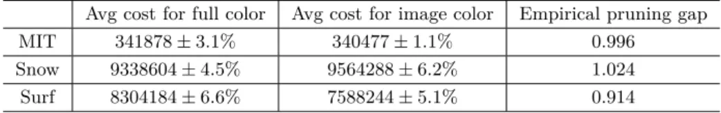
Table 1The empirical values of objective functions for the respective images and algorithms. Avg cost for full color Avg cost for image color Empirical pruning gap
MIT 341878±3.1% 340477±1.1% 0.996
Snow 9338604±4.5% 9564288±6.2% 1.024
Surf 8304184±6.6% 7588244±5.1% 0.914
in other computer vision papers [13]. We use Matlab imnoise function to create noisy images from the original images. We run each instance 20 times, and compute both the average and the variance of the objective function (the variance is due to the random generating process of kd tree).
The results are presented in Figure 1 and Table 1. In Figure 1, one can see that the images produced by the two algorithms are comparable. The full color version seems to preserve a few more details than the image color version, but it also “hallucinates” non-existing colors to minimize the value of the objective function. The visual quality of the de-noised images can be improved by fine-tuning various parameters of the algorithms. We do not report these results here, as our goal was to compare the values of the objective function produced by the two algorithms, as opposed to developing the state of the art de-noising system.
Note that, as per Table 1, for some images the value of the objective function is sometimes
lower for the image color space compared to the full color space. This is because we cannot solve the optimization problem exactly. In particular, using the kd tree to embed the original metric space into a tree metric is an approximate process.
4.1
De-noising with patches
To improve the quality of the de-noised images, we run the experiment forpatches of the image, instead of pixels. Moreover, we use Algorithm 3 which implements not only a pruning step, but also computes the solution directly. In this experiment (see Figure 2 for a sample of the results), each patch (a grid of pixels) from the noisy image is a query point, and the dataset consists of available patches which we use as a substitute for a noisy patch.
In our experiment, to build the dataset, we take one image from the Berkeley segmentation data set, then add noise to the right half of the image, and try to use the patches from the left half to denoise the right half. Each patch is of size 5×5 pixels. We obtain 317×236 patches from the left half of the image and use it as the patch database. Then we apply Algorithm 3 to denoise the image. In particular, for each noisy patch qn (out of 317×237
patches) in the right half of the image, we perform a linear scan to find the closest patchpi
from the patch database, based on the following cost function:
dist(qn, pi) +
X
pj∈neighbor(qn)
dist(pj, pi)
5
wheredist(p, q) is defined to be the sum of squares of thel2 distances between the colors of
corresponding pixels in the two patches.
After that, for each noisy patch we retrieve the closest patch from the patch database. Then for each noisy pixel x, we first identify all the noisy patches (there are at most 25 of them) that cover it. The denoised color of this pixel xis simply the average of all the corresponding pixels in those noisy patches which coverx.
Since the nearest neighbor algorithm is implemented using a linear scan, it takes around 1 hour to denoise one image. One could also apply some more advanced techniques like locality sensitive hashing to find the closest patches with much faster running time.
Figure 1MIT logo (first column, size 45∗124), and two images from the Berkeley segmentation dataset [26] (second & third columns, size 321∗481). The first row shows the original image; the second row shows the noisy image; the third row shows the denoised image using full color space; the fourth row shows the denoised image using image space (our algorithm).
Figure 2 Two images from the Berkeley segmentation dataset [26] (size 321∗481). The first
column shows the original image; the second column shows the half noisy image; the third column shows the de-noised image using our algorithm for the patches.
Acknowledgements. The authors would like to thank Pedro Felzenszwalb for formulating the Simultaneous Nearest Neighbor problem, as well as many helpful discussions about the experimental setup.
References
1 Pankaj K Agarwal, Alon Efrat, and Wuzhou Zhang. Nearest-neighbor searching under uncertainty. In Proceedings of the 32nd symposium on Principles of database systems. ACM, 2012.
2 Alexandr Andoni, Piotr Indyk, Huy L Nguyen, and Ilya Razenshteyn. Beyond locality-sensitive hashing. InProceedings of the Twenty-Fifth Annual ACM-SIAM Symposium on Discrete Algorithms, pages 1018–1028. SIAM, 2014.
3 Aaron Archer, Jittat Fakcharoenphol, Chris Harrelson, Robert Krauthgamer, Kunal Tal-war, and Éva Tardos. Approximate classification via earthmover metrics. In Proceedings of the fifteenth annual ACM-SIAM symposium on Discrete algorithms, pages 1079–1087. Society for Industrial and Applied Mathematics, 2004.
4 Sunil Arya, David M Mount, Nathan S Netanyahu, Ruth Silverman, and Angela Y Wu. An optimal algorithm for approximate nearest neighbor searching fixed dimensions. Journal of the ACM (JACM), 45(6):891–923, 1998.
5 Connelly Barnes, Eli Shechtman, Adam Finkelstein, and Dan Goldman. Patchmatch: A randomized correspondence algorithm for structural image editing. ACM Transactions on Graphics-TOG, 28(3):24, 2009.
6 Jon Louis Bentley. Multidimensional binary search trees used for associative searching.
Communications of the ACM, 18(9):509–517, 1975.
7 Yuri Boykov and Vladimir Kolmogorov. An experimental comparison of min-cut/max-flow algorithms for energy minimization in vision. Pattern Analysis and Machine Intelligence, IEEE Transactions on, 26(9):1124–1137, 2004.
8 Yuri Boykov, Olga Veksler, and Ramin Zabih. Fast approximate energy minimization via graph cuts.Pattern Analysis and Machine Intelligence, IEEE Transactions on, 23(11):1222– 1239, 2001.
9 Gruia Calinescu, Howard Karloff, and Yuval Rabani. Approximation algorithms for the 0-extension problem. SIAM Journal on Computing, 34(2):358–372, 2005.
10 Jittat Fakcharoenphol, Chris Harrelson, Satish Rao, and Kunal Talwar. An improved ap-proximation algorithm for the 0-extension problem. InProceedings of the fourteenth annual ACM-SIAM symposium on Discrete algorithms, pages 257–265. Society for Industrial and Applied Mathematics, 2003.
11 Pedro Felzenszwalb, William Freeman, Piotr Indyk, Robert Kleinberg, and Ramin Zabih. Bigdata: F: Dka: Collaborative research: Structured nearest neighbor search in high di-mensions, 2015. URL:http://cs.brown.edu/~pff/SNN/.
12 Pedro F Felzenszwalb and Daniel P Huttenlocher. Efficient belief propagation for early vision. International journal of computer vision, 70(1):41–54, 2006.
13 Pedro F Felzenszwalb, Gyula Pap, Eva Tardos, and Ramin Zabih. Globally optimal pixel labeling algorithms for tree metrics. InComputer Vision and Pattern Recognition (CVPR), 2010 IEEE Conference on, pages 3153–3160. IEEE, 2010.
14 William T Freeman, Thouis R Jones, and Egon C Pasztor. Example-based super-resolution.
Computer Graphics and Applications, IEEE, 22(2):56–65, 2002.
15 Anupam Gupta, Robert Krauthgamer, and James R Lee. Bounded geometries, fractals, and low-distortion embeddings. In Foundations of Computer Science, 2003. Proceedings. 44th Annual IEEE Symposium on, pages 534–543. IEEE, 2003.
16 Piotr Indyk and Rajeev Motwani. Approximate nearest neighbors: towards removing the curse of dimensionality. InProceedings of the thirtieth annual ACM symposium on Theory of computing, pages 604–613. ACM, 1998.
17 Howard Karloff, Subhash Khot, Aranyak Mehta, and Yuval Rabani. On earthmover dis-tance, metric labeling, and 0-extension.SIAM Journal on Computing, 39(2):371–387, 2009. 18 Alexander V Karzanov. Minimum 0-extensions of graph metrics. European Journal of
Combinatorics, 19(1):71–101, 1998.
19 Jon Kleinberg and Eva Tardos. Approximation algorithms for classification problems with pairwise relationships: Metric labeling and markov random fields. Journal of the ACM (JACM), 49(5):616–639, 2002.
20 Tsvi Kopelowitz and Robert Krauthgamer. Faster clustering via preprocessing. arXiv preprint arXiv:1208.5247, 2012.
21 Robert Krauthgamer and James R Lee. Navigating nets: simple algorithms for prox-imity search. InProceedings of the fifteenth annual ACM-SIAM symposium on Discrete algorithms, pages 798–807. Society for Industrial and Applied Mathematics, 2004.
22 Eyal Kushilevitz, Rafail Ostrovsky, and Yuval Rabani. Efficient search for approximate nearest neighbor in high dimensional spaces. SIAM Journal on Computing, 30(2):457–474, 2000.
23 James R Lee and Assaf Naor. Metric decomposition, smooth measures, and clustering.
Preprint, 2004.
24 Feifei Li, Bin Yao, and Piyush Kumar. Group enclosing queries. Knowledge and Data Engineering, IEEE Transactions on, 23(10):1526–1540, 2011.
25 Yang Li, Feifei Li, Ke Yi, Bin Yao, and Min Wang. Flexible aggregate similarity search. In
Proceedings of the 2011 ACM SIGMOD international conference on management of data, pages 1009–1020. ACM, 2011.
26 David R Martin, Charless C Fowlkes, and Jitendra Malik. Learning to detect natural image boundaries using local brightness, color, and texture cues. Pattern Analysis and Machine Intelligence, IEEE Transactions on, 26(5):530–549, 2004.
27 Man Lung Yiu, Nikos Mamoulis, and Dimitris Papadias. Aggregate nearest neighbor queries in road networks.Knowledge and Data Engineering, IEEE Transactions on, 17(6):820–833, 2005.
A
2
r
+ 1
approximation
Motivated by the importance of ther-sparse graphs in applications, in this section we focus on them and present another algorithm (besides INN) which solves the SNN problem for these graphs. We note that unlike INN, the algorithm presented in this section is not just a pruning step, but it solves the whole SNN problem.
For a graphG= (Q, E) of pseudoarboricityr, let the mapping function bef :E→Q, such that for everye= (qi, qj),f(e) =qi orf(e) =qj, and that for each qi∈Q,|C(qi)| ≤r,
whereC(qi) is defined as{e|f(e) =qi}.
Once we have the mapping functionf, we can run Algorithm 3 to get an approximate solution. Although the naive implementation of this algorithm needsO(rkn) running time, by using the aggregate nearest neighbor algorithm, it can be done much more efficiently. We have the following lemma on the performance of this algorithm.
ILemma 15. If Ghas pseudoarboricityr, the solution of Algorithm 3 gives 2r+ 1 approx-imation to the optimal solution.
Algorithm 3 Algorithm for graph with pseudoarboricityr
InputQuery pointsq1,· · · , qk, the input graphG= (Q, E) with pseudoarboricityr
OutputAn Assignmentp1,· · ·, pk∈P
1: fori= 1tokdo
2: Assignpi←minp∈Pdist(qi, p) +Pj:(qi,qj)∈C(qj)
dist(p,qj)
r+1
3: end for
Proof. Denote the optimal solution asP∗={p∗1,· · ·, p∗k}. We know the optimal cost is Cost(Q, G, P∗) =X i dist(qi, p∗i) + X (qi,qj)∈E dist(p∗i, p∗j) =X i dist(p∗i, qi) + X j:(qi,qj)∈C(qj) dist(p∗i, p∗j)
Let Sol be the solution reported by Algorithm 3. Then we have
Cost(Sol) =X i dist(qi, pi) + X j:(qi,qj)∈C(qj) dist(pi, pj) ≤X i dist(qi, pi) + X j:(qi,qj)∈C(qj) dist(pi, qj) + X j:(qi,qj)∈C(qj) dist(qj, pj)
(by triangle inequality)
≤X i dist(qi, pi) + X j:(qi,qj)∈C(qj) dist(pi, qj) +r X j dist(qj, pj)
(by definition of pseudoarboricity) = (r+ 1)X i dist(qi, pi) + X (qi,qj)∈C(qj) dist(pi, qj) ≤(r+ 1)X i dist(qi, p∗i) + X j:(qi,qj)∈C(qj) dist(p∗i, qj) r+ 1
(by the optimality ofpi in the algorithm)
≤(r+ 1)X i dist(qi, p∗i) + X j:(qi,qj)∈C(qj) dist(p∗i, p∗j) + dist(p∗j, qj) r+ 1
(by triangle inequality)
≤(r+ 1)Cost(Q, G, P∗) +X i X j:(qi,qj)∈C(qj) dist(p∗j, qj) ≤(r+ 1)Cost(Q, G, P∗) +rX j dist(p∗j, qj)
(by definition of pseudoarboricity)
![Figure 2 Two images from the Berkeley segmentation dataset [26] (size 321 ∗ 481). The first column shows the original image; the second column shows the half noisy image; the third column shows the de-noised image using our algorithm for the patches.](https://thumb-us.123doks.com/thumbv2/123dok_us/9321565.2810734/12.892.177.755.765.1016/figure-images-berkeley-segmentation-dataset-original-algorithm-patches.webp)
