This is a repository copy of Assessing uncertainty and complexity in regional-scale crop model simulations.
White Rose Research Online URL for this paper: http://eprints.whiterose.ac.uk/94894/
Version: Accepted Version
Article:
Ramirez-Villegas, J, Koehler, AK orcid.org/0000-0002-1059-8056 and Challinor, AJ orcid.org/0000-0002-8551-6617 (2017) Assessing uncertainty and complexity in regional-scale crop model simulations. European Journal of Agronomy, 88. pp. 84-95. ISSN 1161-0301
https://doi.org/10.1016/j.eja.2015.11.021
© 2015, Elsevier. Licensed under the Creative Commons Attribution-NonCommercial-NoDerivatives 4.0 International http://creativecommons.org/licenses/by-nc-nd/4.0/
[email protected] https://eprints.whiterose.ac.uk/ Reuse
Unless indicated otherwise, fulltext items are protected by copyright with all rights reserved. The copyright exception in section 29 of the Copyright, Designs and Patents Act 1988 allows the making of a single copy solely for the purpose of non-commercial research or private study within the limits of fair dealing. The publisher or other rights-holder may allow further reproduction and re-use of this version - refer to the White Rose Research Online record for this item. Where records identify the publisher as the copyright holder, users can verify any specific terms of use on the publisher’s website.
Takedown
If you consider content in White Rose Research Online to be in breach of UK law, please notify us by
Assessing uncertainty and complexity in regional-scale crop model simulations
Julian Ramirez-Villegas1, 2, 3, *; Ann-Kristin Koehler1; Andrew J. Challinor1, 3
1
Institute for Climate and Atmospheric Science (ICAS), School of Earth and Environment, University of Leeds, Leeds, UK
2
International Center for Tropical Agriculture (CIAT), Cali, Colombia
3
CGIAR Research Program on Climate Change, Agriculture and Food Security (CCAFS)
*Corresponding author
E-mail: [email protected]; [email protected]
Tel (mobile): +44 075 80445592 Fax: +44 113 343 5259
Abstract
Crop models are imperfect approximations to real world interactions between biotic and abiotic factors. In some situations, the uncertainties associated with choices in model
structure, model inputs and parameters can exceed the spatiotemporal variability of simulated yields, thus limiting predictability. For Indian groundnut, we used the General Large Area Model for annual crops (GLAM) with an existing framework to decompose uncertainty, to first understand how skill changes with added model complexity, and then to determine the relevant uncertainty sources in yield and other prognostic variables (total biomass, leaf area index and harvest index). We developed an ensemble of simulations by perturbing GLAM parameters using two different input meteorology datasets, and two model versions that differ in the complexity with which they account for assimilation. We found that added complexity improved model skill, as measured by changes in the root mean squared error (RMSE), by 5-10 % in specific pockets of western, central and southern India, but that 85 % of the
groundnut growing area either did not show improved skill or showed decreased skill from such added complexity. Thus, adding complexity or using overly complex models at regional or global scales should be exercised with caution. Uncertainty analysis indicated that, in situations where soil and air moisture dynamics are the major determinants of productivity, predictability in yield is high. Where uncertainty for yield is high, the choice of weather input data was found critical for reducing uncertainty. However, for other prognostic variables (including leaf area index, total biomass and the harvest index) parametric uncertainty was generally the most important source, with a contribution of up to 90 % in some cases, suggesting that regional-scale data additional to yield to constrain model parameters is needed. Our study provides further evidence that regional-scale studies should explicitly quantify multiple uncertainty sources.
1. Introduction
Crop models are imperfect approximations to real world interactions between biotic and abiotic factors, mainly designed as tools that provide information that is useful for farmers, researchers and policy makers (Affholder et al., 2012; Sinclair and Seligman, 1996). Such information allows making decisions regarding changes in cropping systems at different spatio-temporal scales, with varied degrees of confidence (Challinor et al., 2014). As confidence in crop modelling outcomes depends on the errors and uncertainties associated with the simulation of the system in question, adequately sampling the model and parameter spaces and adequately addressing issues related to data quality and scaling are critical for the delivery of robust information (Kennedy and OÕHagan, 2001; Ramirez-Villegas et al., 2015).
As with environmental models in general, uncertainty in crop modelling arises from the impossibility to model the system (i.e. the cropping system) with complete determinism (Walker et al., 2003). As a result of the ad-hoc nature of crop model development, where models are developed to fit a specific purpose (Affholder et al., 2012), large diversity exists in model structure and complexity (Rivington and Koo, 2011) and hence model structure is a key source of uncertainty (Asseng et al., 2014; Challinor et al., 2014). Lack of precision in parameter values is also an important uncertainty source in crop models. In many modelling applications, calibrated parameters are rarely sufficiently constrained by the available observational data, which is in most cases limited to crop yield and/or phenology (Iizumi et al., 2009), and this results in crop model parameterisations that are incomplete and uncertain (Angulo et al., 2013a). In some cases, parameters are inherited from other models or crops, are assigned values using expert judgment (Tubiello et al., 2007), or are left Ôas defaultÕ [e.g. Jalota et al. (2013) and Lobell et al. (2013)].
Under a variety of situations, the errors and uncertainties associated with choices of crop model structure, parameters, and data sources can exceed the spatiotemporal variability of the system modelled, thus limiting its predictability, particularly when models are used beyond their calibration ranges (Koehler et al., 2013; Li et al., 2015; Montesino-San Martin et al., 2015). For example, variation in simulation dynamics due to varying model structure has been shown to increase as environmental conditions differ more from the observational record (Asseng et al., 2013; Bassu et al., 2014). Similarly, model parameters and model meteorological inputs have been shown to affect the accuracy of simulated yield across a range of conditions (Tao and Zhang, 2013; van Bussel et al., 2011b). Choices in crop model structure or model configuration can also greatly affect the modelling outcomes that underpin decisions (Vermeulen et al., 2013; Weaver et al., 2013).
Remarkably, in spite of the emphasis on error and uncertainty quantification that has accompanied most recent developments in crop modelling (including the increased use of models outside their calibration ranges, e.g. as in climate change impact studies), still only a handful of studies assess multiple uncertainty sources and about one third appropriately address model error by conducting model evaluation [see Ramirez-Villegas et al. (2015) for a review on the topic]. Importantly, with the increased generation of spatially-explicit gridded crop model simulations, not accounting for parametric uncertainty and input data scaling may lead to systematic bias in estimated crop yield responses to temperature and precipitation (Challinor et al., 2015). Thereby, studies comparatively assessing uncertainties arising from model structure, model parameters and input data are warranted.
This work focuses on Indian groundnut and uses the General Large Area Model for annual crops (GLAM, Challinor et al. 2004) in combination with observed yield and weather data to
investigate two key aspects of prediction: complexity and uncertainty. Specifically, we develop a parameter ensemble by perturbing 30 GLAM model parameters using two different input meteorology datasets, and two model versions that differ in the way they account for assimilation. We first analyse yield observations and simulations to determine whether and how skill improves across different regions depending on the different model structures (warranted complexity), and then decompose the variance of simulated historical yield and other model prognostic variables (LAI, biomass, harvest index) to determine the dominant uncertainty sources across the analysis domain. The results of this work contribute insights to enhance understanding of uncertainty in crop simulation at regional scales.
2. Materials and methods
2.1. Study region
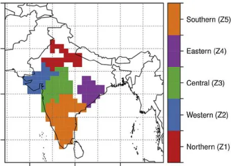
The study area consisted of all 1x1 degree pixels (ca. 100 x 100 km at the Equator) of India where the average cultivated area of groundnut in the period 1966-1990 was greater than 0.2 % (Challinor et al., 2003; Mehrotra, 2011). Following Talawar (2004), we classified all 1x1¼ pixels into one of five groundnut growing zones, which are known to reflect the variation in germplasm grown across India (Fig. 1). These regions receive different amounts of
precipitation during the monsoon season (June to September, when groundnut is primarily grown) and have different prevalent soil types.
2.2. Input data
Daily meteorological inputs required for GLAM are precipitation, downwards shortwave radiation flux and minimum and maximum temperatures. In this study, two sets of these four inputs were used to reflect uncertainty in the choice of input meteorology, as described below.
The first set (referred to as WTH-A) follows the original GLAM formulation of Challinor et al. (2004) and consists of observed daily precipitation data from the Centre for Climate Change Research (CCCR) of the Indian Institute for Tropical Meteorology (IITM) (Rajeevan et al., 2005). We downloaded precipitation data from the CCCR portal
(http://cccr.tropmet.res.in/cccr/home/index.jsp, accessed 1st Sept. 2011) at the native 1x1 degree resolution for the period 1961-2008 (IMD dataset, hereafter). The IMD dataset is based on the interpolation of daily rainfall data from 1,803 rain gauges across India
(Rajeevan et al., 2006, 2005). We obtained maximum and minimum monthly temperatures from the Climatic Research Unit (CRU) dataset at 0.5 degree (CRU-TS3.0 at
http://www.cru.uea.ac.uk/cru/data/hrga, accessed 1st Sept. 2011) (Mitchell and Jones, 2005). We first scaled the CRU data onto the 1x1¼ grid using area-weighted averages and then linearly interpolated to daily values using middle days of the months. Finally, we gathered daily total downwards shortwave solar radiation data from the open-access version of the European Centre for Medium-Range Weather Forecasts (ECMWF) 40+ Reanalysis (ERA-40) (Uppala et al., 2005), available at http://data-portal.ecmwf.int/data/d/era40_daily/ (accessed 1st Sept. 2011) and then scaled it onto the 1x1¼ grid using nearest-neighbour interpolation.
The second set (referred to as WTH-B) is the Water and Global Change (WATCH) Forcing Dataset (WFD), fully described by Weedon et al. (2011). The WFD is a global sub-daily time-step gridded dataset at half-degree resolution for the period 1958-2001, developed by
means of bias correction of the ERA-40 reanalysis. The dataset is of comparable quality to that of Sheffield et al. (2006), and is amongst the gridded datasets used in global and regional crop modelling frameworks (Elliott et al., 2014; Ruane et al., 2015). For a complete
description and analysis of the dataset the reader is referred to Weedon et al. (2011, 2010). We downloaded daily data for total precipitation, downward shortwave radiation, and maximum and minimum temperatures from the WFD website
(https://gateway.ceh.ac.uk/home, accessed 15th June 2013) and aggregated them to the study resolution (1x1 degree).
2.2.2. Soil data
Spatially variable values of permanent wilting point (θll), field capacity (θul) and saturation (θsat) moisture contents were derived from the 30 arc-sec Harmonized World Soil Database (HWSD) (Batjes, 2009; FAO, 2012). The spatially explicit properties in the soil classes occurring within the analysis domain were calculated as the area-weighted-average of each soil profile in each 1x1 grid cell of the analysis grid (see Fig. 1). This resulted in three (one for each soil moisture limit) spatially explicit continuous 1x1 degree datasets that covered the analysis domain. In each grid cell, a GLAM simulation was always associated with its three respective soil moisture content values.
2.2.3. Planting dates
Planting windows used here were those of the global study of Sacks et al. (2010). The dataset of Sacks et al. (2010) is the first global dataset with georeferenced crop planting and
harvesting information. The data were aggregated onto the 1x1 degree analysis grid using area-weighted averages and carefully checked for inconsistencies to ensure planting windows followed the monsoon dynamics.
Figure 1 Study area and agro-ecological classification for model calibration. Growing zone classification was done following Talawar (2004). Only grid cells where GLAM simulations were conducted are shown.
2.2.4. Crop data
We sourced time series of groundnut crop yields, production and harvested area at the district level for the period 1966-1990 from a previous GLAM study (Challinor et al., 2004). The data were first scaled onto the 1x1¼ analysis grid and then carefully checked for reliability both automatically and visually. Whenever a grid cell was composed by fractions of various districts, the yield, production or harvested area of the grid cell was calculated as the
weighted-area average of all districts. Values of zero were removed and marked as missing data where it was obvious that missing data had been wrongly treated as zero (for example when both production and harvested area had been reported as missing). Next, grid cells with more than 20 % missing data or with obvious errors (e.g. all values were equal) in the time series were discarded. A total of 177 grid cells were finally selected for all further analyses, with varying representation of all growing zones (Fig. 1). Out of these 177 grid cells, 27 (15.3
%) were located in the northern zone, 27 (15.3 %) in the western zone, 37 (20.9 %) in the central zone, 25 (14.1 %) in the eastern zone, and 61 (34.4 %) in the southern zone. A more thorough description of these data is provided by Challinor et al. (2004, 2003).
2.3. Crop model description
The General Large Area Model for annual crops (GLAM) is a regional-scale process-based crop model designed to capitalise on the large-scale relationships between climate and crop yields (Challinor et al., 2004). GLAM is a model in which some varietal-level detail is skipped but enough detail is retained to ensure that the weather-yield relationships are captured. GLAM explicitly models the controls of soil water availability, temperature and solar radiation on crop growth, but accounts for nutrition, pests and diseases through a yield gap parameter (CYG), which is constant over time. To some extent, GLAMÕs CYG can also
account for errors in input data (Challinor et al., 2004).
Being less complex than field-scale models, GLAM reduces the risk of
over-parameterisation, while at the same time providing simulations at a variety of spatio-temporal scales. The model is mathematically one-dimensional and simulations can thus be performed at any resolution, provided that crop-climate relationships exist. Some of the drawbacks in GLAM include the difficulty to simulate non-climatic processes which vary over time and that influence crop yields, as well as the risk of input data aggregation error (Challinor et al., 2015; Van Wart et al., 2013). Here, two versions of GLAM were used to understand the importance and impact of added complexity and to quantify structural uncertainty: (1) the original release 2 of the groundnut GLAM model (Challinor, 2009) (referred to as GLAM-TE); and (2) a modified groundnut model version whereby assimilation is computed using a
combination of GLAM-TE with a radiation-use-efficiency (RUE) approach (Osborne et al., 2013) (referred to as GLAM-RUE). Details on both model versions are provided below.
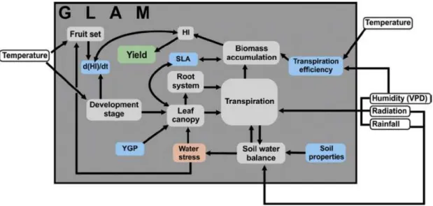
A full description of GLAM is provided elsewhere (Challinor et al., 2004), and therefore the present study only summarises GLAM structure and describes the way both model versions used account for assimilation. Figure 2 shows the structure of the original GLAM model (i.e. GLAM-TE). In GLAM-TE, total crop biomass (∂W/∂t) is estimated on a daily basis using the product of the daily total plant transpiration (TT) and the normalised transpiration efficiency
(ETN) (Eq. 1).
!∀
!# = �&∗ �&) [Eq. 1]
Actual transpiration (TT) is the minimum of three values: (1) the energy-limited transpiration
computed via the Priestley-Taylor equation (Priestley and Taylor, 1972), (2) the water-limited transpiration computed after the potential uptake profile model of Passioura (1983); and (3) the physiologically limited transpiration which depends on the leaf area index (LAI). LAI growth is prescribed by a constant (∂L/∂tmax) and reduced by water stress and the CYG.
The normalised transpiration efficiency (ETN) is the minimum between the parameterised
transpiration efficiency (ET) normalised by the dayÕs vapour pressure deficit (VPD) and a
maximum parameterised value of the normalised transpiration efficiency (ETN, max) (Eq. 2).
�&) = min ./
Figure 2 Structure of the model used in the present study. SLA is specific leaf area, HI is harvest index, ∂HI/∂t is the rate of change in the harvest index, and YGP is the yield gap parameter (CYG). Blue boxes indicate model constants, grey boxes are model prognostics (except yield, which is shown in green), and light orange box indicates intermediate variables. Weather inputs are in hollow rectangles outside the model box. Arrows show flow of information. Adapted from Challinor and Wheeler (2008).
Grain yield (Y) is estimated from total time-integrated biomass (W) and the time-integrated rate of change of harvest index (∂HI/∂t) (Eq. 3).
� = !89 !# �� #< #9 ∗ !∀ !# �� #< #9 = �>∗ � [Eq. 3]
For the GLAM-RUE model, we added an energetic constraint to assimilation such that the biomass production of each day was the minimum between a transpiration-limited and a radiation-limited value (Eq. 4). This modification is based on the fact that well-watered areas often show limited simulation skill if radiation-use constraints to assimilation are not taken into account [see e.g. Keating et al. (2003), and Holzworth et al. (2014)]. More specifically for Indian groundnut, a number of previous studies have shown that rainfall amount and distribution is critical for groundnut production in the north, northwest and west (Bhatia et
al., 2009, 2006; Challinor et al., 2003). In these areas, it has been shown that correlations between solar radiation and crop yield are negative, suggesting that higher solar radiation increases transpirative demand, thus enhancing water stress and lowering yields (Challinor et al., 2005; Ramirez-Villegas, 2014). By contrast, in the states of Andhra Pradesh (south) and Orissa (east), the relationship between crop yields and solar radiation tends to be positive and stronger than that of rainfall; this suggests that these environments can be potentially more limited by radiation availability (as opposed to water). Challinor et al. (2004) showed that GLAM skill in these areas is limited in spite of a strong correlation (>0.8) between simulated biomass and absorbed radiation, implying that energetic constraints to assimilation as
opposed to transpiration alone could be limiting model skill. Based on these earlier findings, we hypothesised that introducing a radiation response function to assimilation in GLAM would improve simulation skill where the radiation-yield relationship was positive and stronger than that of precipitation, whilst maintaining model skill in regions where the converse is true [see discussion section in Challinor et al. (2004)].
In GLAM-RUE, the transpiration-limited component is that of Eq. 1, whereas the radiation-limited one is the product of the parameterised radiation-use efficiency (RUE) and the daily
photosynthetically active radiation (PAR). PAR is computed after Jones et al. (1986), as half the daily intercepted downwards shortwave radiation flux (RSDS) (Eq. 5).
!∀
!# = min �&∗ �&), �Α.∗ ��� [Eq. 4]
where k is the canopy extinction coefficient, parameterised as a constant. This modification resulted in the addition of one equation (Eq. 5) and one parameter (RUE), thus adding
complexity to the original model.
2.4. Crop model calibration and evaluation
In order to calibrate GLAM-TE (GLAM-RUE), the optimal values of 30 (31) `global`
parameters and 1 `local` parameter need to be estimated. The term `global parameter` is used to refer to model parameters that are constant across large and relatively uniform areas (e.g. where duration requirements are known not to vary significantly). The only local parameter in both GLAM-TE and GLAM-RUE is the yield gap parameter (CYG), which is defined
separately for each grid cell. Here, calibration of the global parameters was done per
groundnut growing zone (Fig. 1) by reducing the model error as measured by the root mean squared error (RMSE, Eq. 6) between observed and simulated yield.
���� = Θ9Λ19
Ρ <
9ΣΤ
Υ [Eq. 6]
where O and P refer to observed and predicted quantities of a series of n elements (here, n = 25 years). We used RMSE as it provides a complete measure of the model errors (Taylor, 2001). Calibration of model parameters was done for each combination of GLAM version (GLAM-TE, GLAM-RUE) and input meteorology (WTH-A, WTH-B), as follows:
(1)!First, in order to minimise the interactions between CYG and all other parameters, we
selected the single grid cell with the highest yield per growing zone for the global parameter calibration. This choice assumes that the chosen grid cell reflects potential
on-farm yields for a large and relatively homogeneous region. Following this assumption, this grid cell was assigned a value of CYG=1 throughout all following steps. Choosing a
single grid cell also provided the opportunity to evaluate the skill of the models and their global parameters in areas not used for the global calibration.
(2)!We then developed a parameter ensemble for each growing zone by performing a total of 100 parallel calibration chains, each starting at a different point of the parameter space and with a different order for parameter calibration. Both the starting point and the order of parameter calibration are chosen at random for each chain. In each chain, parameters were calibrated by iteratively testing values within known parameter ranges [see
Supplementary Table S1 for ranges]. As we ran 10 iterations of each chain, this resulted in a total of 30,000 (31,000) calibration runs being performed per growing zone for GLAM-TE (GLAM-RUE). This method is akin to a random sampling of the parameter space [e.g. Beven and Freer (2001); Freer et al. (1996)], but with the difference that it allows a more systematic exploration of the neighbourhood around the starting point of each chain. This process also accounts for co-variation and compensation in model parameter values.
(3)!Next, from all calibration runs we selected all unique global parameter sets below the 25th percentile of RMSE. This value is chosen as a compromise between a number of
parameter sets (often ~1,000) that is computationally feasible but sufficiently large so as to realistically represent both variation in parameter values and model skill. Similar approaches are employed in other methods for parameter estimation, where arbitrary cut-off values are used to select or reproduce parameter sets (Beven and Freer, 2001; Iizumi et al., 2009).
(4)!Finally, for each global parameter set, we performed per grid cell calibration of CYG by
We finally assessed the skill of parameter sets to reproduce observed mean yield and yield variability using a Taylor diagram (Taylor, 2001). In a Taylor diagram, RMSE is decomposed in its three components: mean bias, ratio of standard deviations, and Pearson correlation coefficient (R), thus providing a complete analysis of strengths and flaws in model predictions. Finally, we mapped out the RMSE to show spatial variation in model skill.
2.5. Model complexity and uncertainty analysis
In order to understand whether added complexity in assimilation in GLAM-RUE resulted in a comparative advantage with respect to GLAM-TE, we calculated gains in model skill for each grid cell. To that aim, we first calculated one RMSE value per grid cell and model version as the mean RMSE across all parameter sets and weather inputs, subtracted the mean RMSE of GLAM-RUE from that of GLAM-TE, and then normalised it by the mean RMSE of GLAM-TE (Eq. 7).
����2>ςς = WΞΗ./ΨΛWΞΗ.Ζ[Ψ
WΞΗ./Ψ [Eq. 7]
A positive value in this fractional difference for RMSE indicates that GLAM-RUE had greater model skill compared to GLAM-TE. A bootstrapped t-test with 10,000 replicates was conducted to identify where gains in skill were statistically significant (at α=0.05 and
α=0.10). More specifically, the bootstrapped t-test sampled both parameter sets and weather inputs (the dimensions over which RMSE values in Eq. 7 are averaged) and reported a p-value computed as the ratio of statistically significant bootstrap samples to the total number of replicates. This analysis intended to reveal areas where the additional complexity was indeed warranted.
We define uncertainty as the total variance of a simulated prognostic variable among many model configurations, i.e. combinations of parameter sets, weather input, and GLAM structure. To understand uncertainty and its sources we decomposed total uncertainty of simulated yield, leaf area index, total crop biomass and harvest index into each of its sources following the methods of Hawkins and Sutton (2009) and Vermeulen et al. (2013).
Specifically, uncertainty sources were: (1) parameters, (2) weather inputs, (3) GLAM
structure, and (4) natural variability. Each individual model prediction was fit to a one-degree polynomial loess regression with one degree of smoothing for the entire analysis period (1966-1990). Natural variability was assumed to correspond to the time trend of 5-year running mean residuals of this fit, averaged across all individual model predictions. Using a longer (10-year) running mean produced the same qualitative results. Parametric uncertainty was calculated as the variance of the mean predictions of each parameter set. Similarly, structural uncertainty was the variance of the mean predictions of each model (GLAM-TE and GLAM-RUE). Weather input uncertainty was assumed to be the variance of the mean predictions of WTH-A and WTH-B. Total uncertainty was then calculated as the sum of all sources of uncertainty. The fractional contribution of each source to total uncertainty and its temporal variation was finally calculated. Uncertainty decomposition was performed on the harvested area-weighted mean yield of each growing zone. For a detailed description, analysis and discussion over the assumptions and equations used in our framework to decompose uncertainty, the reader is referred to Hawkins and Sutton (2009).
3. Results
In general, both GLAM versions captured well the spatio-temporal variations of crop yields (Fig. 3, Supplementary Fig. S1). Model skill, however, varied across different growing zones and, for some growing zones (e.g. eastern India), also across parameter sets. The southern region (in orange, Fig. 3) showed the highest overall correlations, primarily due to its sufficient water supply leading to low interannual yield variability (see Supplementary Fig. S1). Skill in this region, as derived from the closeness of each coloured circle to the `perfect` model (hollow circle marked at position 1.0 along the x-axis, Fig. 3) in the Taylor diagram was consistent across model versions and input weather datasets. Similarly, the overall skill of the western (in blue), northern (in red) and central (in green) zones was consistent across weather inputs and GLAM versions. The eastern region (in purple), conversely, showed much larger variation across weather input types and GLAM versions, with WTH-B (i.e. ERA-40 daily bias-corrected data) showing better performance, and small differences between the two model versions for each weather input. More specifically, we note that this is the only region where differences in mean RMSE are large (36.6 % for GLAM-TE and 39.7 % for GLAM-RUE). The remainder of regions showed differences in skill between the two datasets below 10 % (see Supplementary Table S3).
Figure 3 already provides some insight as to the potential effect of the different GLAM versions and, therefore, the potential gains in model skill from the added complexity of GLAM-RUE. For example, in the western zone, GLAM-RUE parameter ensemble members showed less variation in model skill than those of GLAM-TE. In the southern zone, we note a displacement of all parameter sets towards a slightly lower RMSE. A more detailed
investigation of variation in skill across model versions showed that it is mostly these two regions that show gains in skill (Fig. 4). Although gains are relatively low (5-10 %), most of them are statistically significant. In particular, the areas of the western region that border with
Figure 3 Taylor diagrams showing the skill of all parameter sets for each of the growing zones. Standard deviations are normalised to the observations (hence ÒperfectÓ standard deviation is the continuous black arc at 1.0 concentric to the origin). Grey arcs concentric to 1.0 in the x-axis represent the RMSE normalised by the standard deviation of the observations. The skill metrics of each GLAM version, input meteorology, and parameter set are computed using all grid cells and years of the corresponding growing zone. All correlation coefficients are significant at p≤0.001. Color-coding follows Fig. 1.
the central region and some areas in the central region show statistically significant
reductions in RMSE from added complexity. Similar gains in model skill were seen along the eastern coast of the southern region (state of Andhra Pradesh and Tamil Nadu). In the vast majority of India (85 % of the study area), however, the added complexity of GLAM-RUE is
not warranted as either skill gain is not significant or GLAM-RUE causes an increase, sometimes significant, in RMSE with respect to GLAM-TE. Thus, representing assimilation in a more detailed and/or complex manner in an attempt to improve simulation realism did not result in improved groundnut yield simulation skill across most areas of India.
Figure 4 Spatial variation in model skill as measured by the RMSE (in kg ha-1) and in gains in model skill (RMSEDIFF, dimensionless, Eq. 7) from using the more complex GLAM-RUE model. (A) RMSE for GLAM-TE, (B) RMSE for RUE, (C) fractional difference between the RMSE of GLAM-TE and GLAM-RUE (RMSEDIFF), (D) RMSE normalised by observed mean yield for GLAM-TE, and (E) RMSE normalised by observed mean yield for GLAM-RUE. For panel (C): positive values indicate a gain in model skill; black hollow dots indicate significant changes in RMSE at p≤0.1, whereas black filled dots indicate significant gains at p≤0.05 as derived from a bootstrapped t-test.
3.2. Uncertainties at the regional scale
For yield, Fig. 5 shows the fractional uncertainty partitioned by source, whereas Fig. 6 shows the absolute uncertainty values for each source. In general total absolute uncertainty in yield
was the lowest in central and southern India, as interannual variability was low, and
agreement between simulations of different input types was greater than for all other zones (also see Supplementary Fig. S2). Across all growing zones, the choice of weather input types (blue areas in Fig. 5) was the most important uncertainty source for yield, albeit with varying importance in time and space. We note three different patterns of variation in the contribution of weather input types to total uncertainty. First, a monotonic reduction during the analysis period was observed in northern India, mostly as a result of growing agreement between yield simulations (see Supplementary Fig. S2). Second, a sharp reduction followed by an equally sharp increase and then a plateauing was seen in western, eastern and southern India, although the time at which the local minimum is reached is different for each region (early in the analysis period for the west and south, and late for the east). And third, in central India, a monotonic increase until a local maximum and then a monotonic decrease was observed, primarily as a result of increasing absolute differences between simulations with different input types, but also due to a concomitant decrease in the difference between different GLAM versions (see Supplementary Fig. S2C).
For yield, parametric uncertainty was generally not a major uncertainty source, particularly when compared with natural variability and uncertainty from weather inputs. Nevertheless, for biomass, harvest index and LAI, the total uncertainty was larger than for yield. Parameter uncertainty was the largest contributor to total uncertainty, with 50-80 % of total variation (Supplementary Figs. S3-S5). This larger contribution is a result of optimising and calibrating the model to correctly simulate yield, and leaving all other model outputs unconstrained. That is, parameters directly affecting LAI such as the prescribed rate of leaf growth (∂L/∂tmax) and the yield gap parameter (CYG) would have large variation across the parameter ensemble and
Figure 5 Fractional uncertainty in regional yield during the period 1966-1990, decomposed by source. Shown is the contribution of four different sources to total yield variance, namely, weather inputs (blue), GLAM structure (dark green), parameter sets (light green), and natural variability (orange).
(though not solely) affected by the transpiration efficiency, the maximum transpiration efficiency, the radiation-use efficiency (only in GLAM-RUE), and the crop duration; and the harvest index, which is mainly defined by the prescribed rate of increase in the harvest index (∂HI/∂t) and the duration from start of pod filling to physiological maturity. Values for all these parameters showed large variation, often spanning the full range along which the
Figure 6 Absolute uncertainty (standard deviation) in regional yield during the period 1966-1990, decomposed by source. Shown is the uncertainty in yield stemming from four different sources, namely, weather inputs (blue), GLAM structure (dark green), parameter sets (light green), and natural variability (orange). Note the differences in y-axis scale across panels, deliberately chosen to highlight differences between absolute uncertainties from all sources within each zone.
parameter was allowed to vary (Table S1). Additionally, although with exceptions in specific zones and prognostic variables (e.g. all variables in northern India, and yield in southern India), parametric uncertainty was higher for GLAM-RUE as compared to GLAM-TE,
suggesting increased parameter interactions in GLAM-RUE and hence highlighting the compensatory nature of parameters in process-based models (see Supplementary Fig. S6).
A further analysis of correlation with the full ensemble of parameters for both weather input types separately for each GLAM version confirmed the compensatory nature of model parameters and their errors. Specifically, those parameters directly related to assimilation, that is, the maximum transpiration efficiency (ETN, max), the normalised transpiration efficiency (TE), the rate of change in the harvest index (∂HI/∂t), the maximum rate of transpiration (TTmax) and the duration of the grain filling stage are negatively, albeit not
strongly (i.e. correlation between -0.2 and -0.35, p≤0.001), associated with the prescribed rate of leaf growth (∂L/∂tmax). The maximum rate of transpiration was also negatively associated with the remainder of growth parameters, but particularly so with the maximum transpiration efficiency (R=-0.47), the crop and soil albedo (R=-0.42) and the rate of root growth (R =-0.62). These relationships were consistent for the two GLAM versions.
4. Discussion
4.1. Limits to GLAM ensemble skill in simulating groundnut yields
GLAM reproduced mean yields and (to a lesser extent) interannual yield variability (Figs. 3-4, Supplementary Fig. S1). In western India, however, there was a remarkably good
simulation of extreme yield values from the parameter ensemble, with only three out of the 25 years being outside the ensemble predicted ranges (Supplementary Fig. S1). However, even with a thorough sampling of the parameter space, fully capturing observations was not possible. This result is in broad agreement with previous studies, which show that yield observations sometimes fall outside parameter ensemble simulations (Iizumi et al., 2011; Tao et al., 2009). Errors in the observed yield data and its scaling to the analysis grid, errors of the
assumed planting calendars and soil types, errors from assuming constant pest and disease pressures and nitrogen limitations by assuming CYG to be constant over time, or errors in
model structure beyond the modifications introduced here are the most likely causes for these limitations. Previous work with GLAM has shown that errors in yield measurements can have a comparable impact to that of errors in input meteorology (Watson and Challinor, 2013).
GLAM has been previously reported to simulate interannual variability with limitations in some areas (Challinor et al., 2007), with varying factors being potential causes. Here, we note that the limited GLAM skill in northern Gujarat (western India) was related to a very low harvested area, mostly nearby the wetter zones of southern Gujarat, which by contrast shows much higher harvested area and yield. The larger scale of the observed yield data compared to the scale of the GLAM simulations in these areas led to associating very low rainfall grid cells (towards the Rajasthan desert) to relatively high yields. Limited skill in regions with low harvested area has also been reported elsewhere (Watson et al., 2015). In fact, at the regional scale, yield simulations showed better performance in the largest producing regions (western, southern) as compared to for example the north or the centre, where harvested area is lower (see Supplementary Fig. S1). Grid cells with a significant share of ocean also suffered from scaling-related errors (see western coasts in Fig. 4). Similar behaviour would be expected where large variations in harvested area occur over relatively short geographical distances Ð which we did not assess here (but see Watson et al., 2014).
Missing processes related to soil nutrient availability and pests and diseases which might change over time depending on farmerÕs management strategies, all of which are
simplistically accounted for by a non-time-varying CYG, may have also constrained the
remains a topic meriting more research, as it is not clear whether or how complexity of biotic and abiotic stress interactions changes across scale and time. Importantly, as was shown here, adding complexity to the crop model is not always warranted, and should therefore be
exercised with caution (see below).
4.2. Added complexity no guarantee of greater model skill
Our results indicate that only a small part (ca. 15 %) of the study area showed statistically significant improvements (5-10 %) in model skill as a result of added complexity in simulating assimilation. However, we also found significant skill loss in a number of
situations (53 % of grid cells, p ≤ 0.1). Importantly, skill gains and losses were not restricted to water-limited areas (e.g. western and northern India), indicating that model skill changes are the product of interactions at the process level between various factors and model
parameters, or that the modifications introduced to GLAM-RUE do not capture well the main limiting factors of crop productivity. Our analysis demonstrates that the thorough testing of changes in process-based model structure against available observations should become standard practice in crop modelling [e.g. van Oort et al. (2015)].
The fact that skill gains in the range of 5-10 % occurred is encouraging, however, the fact that such gains occurred only in specific areas or that there was skill loss suggests that careful assessments of model structure are required when structural changes to the model are being done. This result is consistent with previous research where increased simulation detail did not necessarily improve model skill (Adam et al., 2011). Importantly, our results, in line with those of Challinor et al. (2014), open up an interesting debate on the unwarranted complexity in crop models for both regional- and field-scale applications. More specifically, regardless of the spatial scale they have been designed for, models have been found to hold more
complexity than can be constrained by using available observations (Asseng et al., 2013; Challinor et al., 2014). This may, at least in part, explain why large uncertainties occur in relatively un-calibrated global crop model simulations (Rosenzweig et al., 2014).
Methodologies that aid in building appropriate modelling solutions for specific problems may provide ways to define optimal model structures across scales (Adam et al., 2012, 2010; Affholder et al., 2012). However, at the regional scale, the only available data is often crop yield (but see Iizumi et al. 2009), which would preclude the assessment of individual (e.g. leaf area, soil water dynamics) crop model components.
We note that while the use of a radiation-use efficiency approach may still be an over-simplification of assimilation (Adam et al., 2011), the combination of water and radiation constraints to assimilation even in the simplistic fashion described here is considered realistic (Holzworth et al., 2014; Keating et al., 2003). Furthermore, the way GLAM-RUE accounts for assimilation is arguably both more complex and realistic than that of GLAM-TE, which computes assimilation using only water limitations. Hence, the expectation is that GLAM-RUE would perform better, particularly where radiation limitations dominate over water limitations. Our comparison between the two model versions thus provides a clear quantitative assessment of the effects of the hypothesised effects of increased model complexity.
4.3. Uncertainties in regional-scale simulations
We used a previously established framework (Hawkins and Sutton, 2009) to partition uncertainty in an ensemble of regional groundnut crop simulations based on two versions of the GLAM model, two different input weather datasets previously used for crop simulations (Challinor et al., 2004; Ruane et al., 2015), and a parameter ensemble. We found that
uncertainties in simulated regional yield were different in both extent and fractional
contributions to the uncertainties in other model outputs such as leaf area index, harvest index and total crop biomass. Thus, low yield uncertainty occurs at the expense of high uncertainty in the remainder of model outputs, which was further confirmed by the large variation in parameter values as well as, for example, the associations between assimilation and leaf dynamics parameters (see Sect. 3.2). Additional observational constraints, therefore, will be essential to reduce uncertainty in both yield and in other model prognostic variables, as well as to be able to appropriately tie the model processes to the sites and scales of analysis (also see Challinor et al. 2014; Ramirez-Villegas et al. 2015).
The estimates of yield uncertainty provided here in general point to large spatio-temporal differences in the uncertainty stemming from the different sources, as well as to particular situations where predictability increases due to decreasing total uncertainty and, more specifically, meteorological input uncertainty. For western India, we found this greater predictability (occurring during 1970-1975) to be associated with water dynamics (seasonal mean precipitation, evapotranspiration and water uptake), and to a lesser extent similarity in simulated crop duration. For eastern India, greater predictability occurred during 1980-1985, and was associated with seasonal mean precipitation, soil water dynamics and high similarity in VPD. In southern India, high predictability (1965-1975) was primarily associated with similarity in soil water dynamics simulation across the ensemble of runs even if seasonal mean precipitation and crop duration differed across input weather datasets and GLAM versions (data not shown). Although our simulations were based only on GLAM, and would hence tend to underestimate structural uncertainty, this result heightens the importance of using meteorological forcing datasets that are observation-based and reflect well the real
values of the variables that influence the system, which can vary geographically (van Bussel et al., 2011a, 2011b; Watson and Challinor, 2013).
Moreover, particularly for regional- and global-scale crop simulations, where fully observational data sources at daily scale for performing crop simulations are lacking, this results stresses the importance of quantifying the uncertainty stemming from the use of different freely available data sources (Angulo et al., 2013b; Ruane et al., 2015). Future efforts should also concentrate on improving methods for bias correction of modelled climate data, as a key input for regional studies in areas with limited availability of observational data.
Parameter uncertainty, similar to other types of environmental modelling approaches (Beven, 2006; Stainforth et al., 2005), was found to be an important aspect of groundnut growth prediction. Particularly for predictions of LAI, biomass and the harvest index, parameter uncertainty is by far the most important uncertainty source, with a contribution of up to 90 % in some cases. Parametric uncertainty is also a relevant topic for climate change impact assessments (Iizumi et al., 2014a, 2011). In this study, the construction of a parameter ensemble allowed to better capture variability, mainly through the ensemble mean and its variance (Supplementary Fig. S1). We argue that a substantial part of these uncertainties can be reduced, particularly as models improve their predictive ability through extensive testing and improvement against observational data (Asseng et al., 2014, 2013; Challinor et al., 2014), as regional-scale understanding of processes improves (Challinor et al., 2015; Iizumi et al., 2014a), and as improved regional and global-scale crop and meteorological datasets become available (Iizumi et al., 2014b; Van Wart et al., 2015). Extending the work presented here to include other crop models and input yield and meteorology datasets could further
provide insights as additional entry points for uncertainty reduction for the simulation of groundnut productivity at the regional scale.
5. Conclusions
In the present study, we assessed two important aspects of crop growth and yield prediction. Firstly, we assessed the benefit from adding complexity to the crop model. Our relatively minor modification to the way the GLAM model accounts for assimilation (from only water-limited to both radiation- and water-water-limited) resulted in improvements in model error in the range 5-10 % (as measured by changes in the RMSE). These improvements, however, were restricted to specific regions and occurred in only ca. 15 % of the study area. Such
improvements, as would be expected, occurred in radiation-limited environments (southern India). However, skill improvements were also seen in highly water-limited areas (north-western), and decreases in skill were found in other parts where we would have expected either no change in skill or an improvement in skill. Based on these results, we suggest that process-based model improvement efforts thoroughly assess the impacts of changes in model structure on model skill, simulation realism and uncertainty. More broadly, our results also imply that the use of overly complex site-based crop models at the regional or global scale may not be warranted, or even be misleading. Whilst only further work will help determining whether the findings herein presented apply to other regions and crops, the methodology presented here can provide a basis to test effects of increased complexity on model skill. Future studies may extend the methods used here to test the effect of changes in entire sub-modules (e.g. water or nutrient dynamics) on the skill of multiple output variables, for example.
Secondly, we assessed uncertainties in an ensemble of crop simulations. Our findings indicate that for reducing simulated yield uncertainty, the choice of input weather data is critical. Despite uncertainty, low total uncertainty and hence high predictability occurred when yield was primarily limited by either air or soil moisture. In contrast to what was found for yield, we found that reducing uncertainty in other prognostic variables such as LAI, biomass and the harvest index may require a more crop-observation-intensive approach, as parameter uncertainty was found to be the most important uncertainty source. Although we used a single model (GLAM) as well as a modified version of it, the fact that this finding is
consistent across the prognostic variables and growing zones analysed suggests that targeted reduction in parameter uncertainty, and, in particular, of those parameters that have large influence in yield and are related to one another (leaf area growth rate, harvest index rate of increase, transpiration efficiencies, and grain filling duration) is needed. In the absence of observations to constrain model parameters, we argue that future regional-scale studies should consider this uncertainty source explicitly in their simulations. Additionally, the analysis framework used here may provide a basis for not only quantifying but understanding uncertainty and its main sources.
Appendix (list of symbols and acronyms, also see Supplementary Tables S1-S2)
∂L/∂tmax: Maximum rate of change in leaf area index (LAI) (day-1)
∂HI/∂t: Rate of change in the harvest index (day-1)
: Soil volumetric moisture content at permanent wilting point (fraction) : Soil volumetric moisture content at field capacity (fraction)
: Soil volumetric moisture content at saturation (fraction) CYG: Yield gap parameter (fraction of LAI)
ETN, max: Maximum normalised transpiration efficiency (g kg-1) HI: Harvest index (dimensionless)
LAI: Leaf area index (m2 m-2)
R: Correlation coefficient (dimensionless)
ll θ ul θ sat θ
RMSE: Root mean square error (units of variable being assessed, e.g. crop yield: kg ha-1) TE: Transpiration efficiency (Pa)
TT: Total daily transpiration (cm day-1)
TTmax: Maximum rate of transpiration (cm day-1) VPD: Vapour pressure deficit (kPa)
Acknowledgments
This work was supported by the CGIAR Research Program on Climate Change, Agriculture and Food Security (CCAFS). Authors thank all current members of the Climate Impacts Group at University of Leeds and former member Dr. James Watson for insightful discussions on uncertainty and scaling issues. Authors thank Ed Hawkins for advice on uncertainty analysis. JRV thanks David Arango from the International Center for Tropical Agriculture (CIAT) for statistical advice. We thank two anonymous reviewers for their comments during the review process.
References
Adam, M., Belhouchette, H., Corbeels, M., Ewert, F., Perrin, A., Casellas, E., Celette, F., Wery, J., 2012. Protocol to support model selection and evaluation in a modular crop modelling framework: An application for simulating crop response to nitrogen supply. Comput. Electron. Agric. 86, 43Ð54.
Adam, M., Ewert, F., Leffelaar, P.A., Corbeels, M., van Keulen, H., Wery, J., 2010.
CROSPAL, software that uses agronomic expert knowledge to assist modules selection for crop growth simulation. Environ. Model. Softw. 25, 946Ð955.
Adam, M., Van Bussel, L.G.J., Leffelaar, P.A., Van Keulen, H., Ewert, F., 2011. Effects of modelling detail on simulated potential crop yields under a wide range of climatic conditions. Ecol. Modell. 222, 131Ð143.
Affholder, F., Tittonell, P., Corbeels, M., Roux, S., Motisi, N., Tixier, P., Wery, J., 2012. Ad Hoc Modeling in Agronomy: What Have We Learned in the Last 15 Years? Agron. J. 104, 735Ð748.
Angulo, C., Rštter, R., Lock, R., Enders, A., Fronzek, S., Ewert, F., 2013a. Implication of crop model calibration strategies for assessing regional impacts of climate change in Europe. Agric. For. Meteorol. 170, 32Ð46.
Angulo, C., Rštter, R., Trnka, M., Pirttioja, N., Gaiser, T., Hlavinka, P., Ewert, F., 2013b. Characteristic ÒfingerprintsÓ of crop model responses to weather input data at different spatial resolutions. Eur. J. Agron. 49, 104Ð114.
Asseng, S., Ewert, F., Martre, P., Rštter, R.P., Lobell, D.B., Cammarano, D., Kimball, B.A., Ottman, M.J., Wall, G.W., White, J.W., Reynolds, M.P., Alderman, P.D., Prasad, P.V. V., Aggarwal, P.K., Anothai, J., Basso, B., Biernath, C., Challinor, A.J., De Sanctis, G., Doltra, J., Fereres, E., Garcia-Vila, M., Gayler, S., Hoogenboom, G., Hunt, L.A.,
Izaurralde, R.C., Jabloun, M., Jones, C.D., Kersebaum, K.C., Koehler, A.-K., MŸller, C., Naresh Kumar, S., Nendel, C., OÕLeary, G., Olesen, J.E., Palosuo, T., Priesack, E., Eyshi Rezaei, E., Ruane, A.C., Semenov, M.A., Shcherbak, I., Stšckle, C.,
Stratonovitch, P., Streck, T., Supit, I., Tao, F., Thorburn, P.J., Waha, K., Wang, E., Wallach, D., Wolf, J., Zhao, Z., Zhu, Y., 2014. Rising temperatures reduce global wheat production. Nat. Clim. Chang. 5, 143Ð147.
Asseng, S., Ewert, F., Rosenzweig, C., Jones, J.W., Hatfield, J.L., Ruane, A.C., Boote, K.J., Thorburn, P.J., Rštter, R.P., Cammarano, D., Brisson, N., Basso, B., Martre, P.,
Aggarwal, P.K., Angulo, C., Bertuzzi, P., Biernath, C., Challinor, A.J., Doltra, J., Gayler, S., Goldberg, R., Grant, R., Heng, L., Hooker, J., Hunt, L.A., Ingwersen, J., Izaurralde, R.C., Kersebaum, K.C., MŸller, C., Naresh Kumar, S., Nendel, C., OÕLeary, G., Olesen, J.E., Osborne, T.M., Palosuo, T., Priesack, E., Ripoche, D., Semenov, M.A., Shcherbak, I., Steduto, P., Stšckle, C., Stratonovitch, P., Streck, T., Supit, I., Tao, F., Travasso, M., Waha, K., Wallach, D., White, J.W., Williams, J.R., Wolf, J., 2013. Uncertainty in simulating wheat yields under climate change. Nat. Clim. Chang. 3, 827Ð 832.
Bassu, S., Brisson, N., Durand, J.-L., Boote, K., Lizaso, J., Jones, J.W., Rosenzweig, C., Ruane, A.C., Adam, M., Baron, C., Basso, B., Biernath, C., Boogaard, H., Conijn, S., Corbeels, M., Deryng, D., De Sanctis, G., Gayler, S., Grassini, P., Hatfield, J., Hoek, S., Izaurralde, C., Jongschaap, R., Kemanian, A.R., Kersebaum, K.C., Kim, S.-H., Kumar, N.S., Makowski, D., MŸller, C., Nendel, C., Priesack, E., Pravia, M.V., Sau, F.,
Shcherbak, I., Tao, F., Teixeira, E., Timlin, D., Waha, K., 2014. How do various maize crop models vary in their responses to climate change factors? Glob. Chang. Biol. 20, 2301Ð2320.
Batjes, N.H., 2009. Harmonized soil profile data for applications at global and continental scales: updates to the WISE database. Soil Use Manag. 25, 124Ð127.
Beven, K., 2006. A manifesto for the equifinality thesis. J. Hydrol. 320, 18Ð36.
Beven, K., Freer, J., 2001. Equifinality , data assimilation , and uncertainty estimation in mechanistic modelling of complex environmental systems using the GLUE
methodology. J. Hydrol. 249, 11Ð29.
Bhatia, V.S., Singh, P., Kesava Rao, A.V.R., Srinivas, K., Wani, S.P., 2009. Analysis of Water Non-limiting and Water Limiting Yields and Yield Gaps of Groundnut in India Using CROPGRO-Peanut Model. J. Agron. Crop Sci. 195, 455Ð463.
Bhatia, V.S., Singh, P., Wani, S.P., Kesava Rao, A.V.R., Srinivas, K., 2006. Yield Gap Analysis of Soybean, Groundnut, Pigeonpea and Chickpea in India Using Simulation Modeling. Global Theme on Agroecosystems Report no. 31. International Crops Research Institute for the Semi-Arid Tropics (ICRISAT), Patancheru 502 324, Andhra Pradesh, India.
Challinor, A., Martre, P., Asseng, S., Thornton, P., Ewert, F., 2014. Making the most of climate impacts ensembles. Nat. Clim. Chang. 4, 77Ð80.
Challinor, A.J., 2009. General Large-Area Model for annual crops (GLAM) Documentation for Release 2. Institute for Climate and Atmospheric Science, School of Earth and Environment, University of Leeds, Leeds, UK.
Challinor, A.J., Parkes, B., Ramirez-Villegas, J., 2015. Crop yield response to climate change varies with cropping intensity. Glob. Chang. Biol. 21, 1679Ð1688.
Combined Seasonal Weather and Crop Productivity Forecasting System: Determination of the Working Spatial Scale. J. Appl. Meteorol. 42, 175Ð192.
Challinor, A.J., Wheeler, T.R., 2008. Use of a crop model ensemble to quantify CO2 stimulation of water-stressed and well-watered crops. Agric. For. Meteorol. 148, 1062Ð 1077.
Challinor, A.J., Wheeler, T.R., Craufurd, P.Q., Ferro, C.A.T., Stephenson, D.B., 2007.
Adaptation of crops to climate change through genotypic responses to mean and extreme temperatures. Agric. Ecosyst. Environ. 119, 190Ð204.
Challinor, A.J., Wheeler, T.R., Craufurd, P.Q., Slingo, J.M., Grimes, D.I.F., 2004. Design and optimisation of a large-area process-based model for annual crops. Agric. For. Meteorol. 124, 99Ð120.
Challinor, A.J., Wheeler, T.R., Slingo, J.M., Craufurd, P.Q., Grimes, D.I.F., 2005. Simulation of Crop Yields Using ERA-40: Limits to Skill and Nonstationarity in WeatherÐYield Relationships. J. Appl. Meteorol. 44, 516Ð531.
Elliott, J., MŸller, C., Deryng, D., Chryssanthacopoulos, J., Boote, K.J., BŸchner, M., Foster, I., Glotter, M., Heinke, J., Iizumi, T., Izaurralde, R.C., Mueller, N.D., Ray, D.K.,
Rosenzweig, C., Ruane, A.C., Sheffield, J., 2014. The Global Gridded Crop Model intercomparison: data and modeling protocols for Phase 1 (v1.0). Geosci. Model Dev. Discuss. 7, 4383Ð4427.
FAO, 2012. Harmonized World Soil Database (version 1.2). FAO, Rome, Italy and IIASA, Laxenburg, Austria.
Freer, J., Beven, K., Ambroise, B., 1996. Bayesian Estimation of Uncertainty in Runoff Prediction and the Value of Data: An Application of the GLUE Approach. Water Resour. Res. 32, 2161Ð2173.
Hawkins, E., Sutton, R., 2009. The Potential to Narrow Uncertainty in Regional Climate Predictions. Bull. Am. Meteorol. Soc. 90, 1095Ð1107.
Holzworth, D.P., Huth, N.I., DeVoil, P.G., Zurcher, E.J., Herrmann, N.I., McLean, G., Chenu, K., van Oosterom, E.J., Snow, V., Murphy, C., Moore, A.D., Brown, H., Whish, J.P.M., Verrall, S., Fainges, J., Bell, L.W., Peake, A.S., Poulton, P.L., Hochman, Z., Thorburn, P.J., Gaydon, D.S., Dalgliesh, N.P., Rodriguez, D., Cox, H., Chapman, S., Doherty, A., Teixeira, E., Sharp, J., Cichota, R., Vogeler, I., Li, F.Y., Wang, E., Hammer, G.L., Robertson, M.J., Dimes, J.P., Whitbread, A.M., Hunt, J., van Rees, H., McClelland, T., Carberry, P.S., Hargreaves, J.N.G., MacLeod, N., McDonald, C., Harsdorf, J., Wedgwood, S., Keating, B.A., 2014. APSIM Ð Evolution towards a new generation of agricultural systems simulation. Environ. Model. Softw. 62, 327Ð350. Iizumi, T., Tanaka, Y., Sakurai, G., Ishigooka, Y., Yokozawa, M., 2014a. Dependency of
parameter values of a crop model on the spatial scale of simulation. J. Adv. Model. Earth Syst. 6, 527Ð540.
Iizumi, T., Yokozawa, M., Nishimori, M., 2009. Parameter estimation and uncertainty
analysis of a large-scale crop model for paddy rice: Application of a Bayesian approach. Agric. For. Meteorol. 149, 333Ð348.
Iizumi, T., Yokozawa, M., Nishimori, M., 2011. Probabilistic evaluation of climate change impacts on paddy rice productivity in Japan. Clim. Change 107, 391Ð415.
Iizumi, T., Yokozawa, M., Sakurai, G., Travasso, M.I., Romanenkov, V., Oettli, P., Newby, T., Ishigooka, Y., Furuya, J., 2014b. Historical changes in global yields: major cereal
and legume crops from 1982 to 2006. Glob. Ecol. Biogeogr. 23, 346Ð357.
Jalota, S.K., Kaur, H., Kaur, S., Vashisht, B.B., 2013. Impact of climate change scenarios on yield, water and nitrogen-balance and -use efficiency of riceÐwheat cropping system. Agric. Water Manag. 116, 29Ð38.
Jones, C.A., Kiniry, J.R., Dyke, P.T., 1986. CERES-Maize: a simulation model of maize growth and development. Texas A&M University Press.
Keating, B.A., Carberry, P.S., Hammer, G.L., Probert, M.E., Robertson, M.J., Holzworth, D., Huth, N.I., Hargreaves, J.N.G., Meinke, H., Hochman, Z., McLean, G., Verburg, K., Snow, V., Dimes, J.P., Silburn, M., Wang, E., Brown, S., Bristow, K.L., Asseng, S., Chapman, S., McCown, R.L., Freebairn, D.M., Smith, C.J., 2003. An overview of APSIM, a model designed for farming systems simulation. Eur. J. Agron. 18, 267Ð288. Kennedy, M.C., OÕHagan, A., 2001. Bayesian calibration of computer models. J. R. Stat. Soc.
Ser. B (Statistical Methodol. 63, 425Ð464.
Koehler, A.-K., Challinor, A.J., Hawkins, E., Asseng, S., 2013. Influences of increasing temperature on Indian wheat: quantifying limits to predictability. Environ. Res. Lett. 8, 34016.
Li, T., Hasegawa, T., Yin, X., Zhu, Y., Boote, K., Adam, M., Bregaglio, S., Buis, S., Confalonieri, R., Fumoto, T., Gaydon, D., Marcaida, M., Nakagawa, H., Oriol, P., Ruane, A.C., Ruget, F., Singh, B.-, Singh, U., Tang, L., Tao, F., Wilkens, P., Yoshida, H., Zhang, Z., Bouman, B., 2015. Uncertainties in predicting rice yield by current crop models under a wide range of climatic conditions. Glob. Chang. Biol. 21, 1328Ð1341. Lobell, D.B., Hammer, G.L., McLean, G., Messina, C., Roberts, M.J., Schlenker, W., 2013.
The critical role of extreme heat for maize production in the United States. Nat. Clim. Chang. 3, 497Ð501.
Mehrotra, N., 2011. Groundnut, Commodity Specific Study. Department of Economic Analysis and Research, National Bank for Agriculture and Rural Development, Mumbai, India.
Mitchell, T.D., Jones, P.D., 2005. An improved method of constructing a database of monthly climate observations and associated high-resolution grids. Int. J. Climatol. 25, 693Ð712. Montesino-San Martin, M., Olesen, J.E., Porter, J.R., 2015. Can crop-climate models be
accurate and precise? A case study for wheat production in Denmark. Agric. For. Meteorol. 202, 51Ð60.
Osborne, T., Rose, G., Wheeler, T., 2013. Variation in the global-scale impacts of climate change on crop productivity due to climate model uncertainty and adaptation. Agric. For. Meteorol. 170, 183Ð194.
Passioura, J.B., 1983. Roots and drought resistance. Agric. Water Manag. 7, 265Ð280. Priestley, C.H.B., Taylor, R.J., 1972. On the Assessment of Surface Heat Flux and
Evaporation Using Large-Scale Parameters. Mon. Weather Rev. 100, 81Ð92.
Rajeevan, M., Bhate, J., Kale, J.D., Lal, B., 2005. Development of a High Resolution Daily Gridded Rainfall Data for the Indian Region, Met. Monograph Climatology No. 22/2005. National Climate Centre, India Meteorological Department, Government of India, Pune, India.
Rajeevan, M., Bhate, J., Kale, J.D., Lal, B., 2006. High resolution daily gridded rainfall data for the India region: Analysis of break and active monsoon spells. Curr. Sci. 91, 296Ð 306.
Ramirez-Villegas, J., 2014. Genotypic adaptation of Indian groundnut to climate change: an ensemble approach. University of Leeds.
Ramirez-Villegas, J., Watson, J., Challinor, A.J., 2015. Identifying traits for genotypic adaptation using crop models. J. Exp. Bot. 66, 3451Ð3462.
Rivington, M., Koo, J., 2011. Report on the Meta-Analysis of Crop Modelling for Climate Change and Food Security Survey. CGIAR Research Program on Climate Change, Agriculture and Food Security.
Rosenzweig, C., Elliott, J., Deryng, D., Ruane, A.C., MŸller, C., Arneth, A., Boote, K.J., Folberth, C., Glotter, M., Khabarov, N., Neumann, K., Piontek, F., Pugh, T. a M., Schmid, E., Stehfest, E., Yang, H., Jones, J.W., 2014. Assessing agricultural risks of climate change in the 21st century in a global gridded crop model intercomparison. Proc. Natl. Acad. Sci. U. S. A. 111, 3268Ð73.
Ruane, A.C., Goldberg, R., Chryssanthacopoulos, J., 2015. Climate forcing datasets for agricultural modeling: Merged products for gap-filling and historical climate series estimation. Agric. For. Meteorol. 200, 233Ð248.
Sacks, W.J., Deryng, D., Foley, J.A., Ramankutty, N., 2010. Crop planting dates: an analysis of global patterns. Glob. Ecol. Biogeogr. 19, 607Ð620.
Sheffield, J., Goteti, G., Wood, E.F., 2006. Development of a 50-Year High-Resolution Global Dataset of Meteorological Forcings for Land Surface Modeling. J. Clim. 19, 3088Ð3111.
Sinclair, T.R., Seligman, N.G., 1996. Crop Modeling: From Infancy to Maturity. Agron. J. 88, 698Ð704.
Stainforth, D.A., Aina, T., Christensen, C., Collins, M., Faull, N., Frame, D.J.,
Kettleborough, J.A., Knight, S., Martin, A., Murphy, J.M., Piani, C., Sexton, D., Smith, L.A., Spicer, R.A., Thorpe, A.J., Allen, M.R., 2005. Uncertainty in predictions of the climate response to rising levels of greenhouse gases. Nature 433, 403Ð406.
Talawar, S., 2004. Peanut in India: History, Production and Utilization, Peanut in Local and Global Food Systems Series Report No. 5. University of Georgia, Athens, Georgia, USA.
Tao, F., Zhang, Z., 2013. Climate change, wheat productivity and water use in the North China Plain: A new super-ensemble-based probabilistic projection. Agric. For. Meteorol. 170, 146Ð165.
Tao, F., Zhang, Z., Liu, J., Yokozawa, M., 2009. Modelling the impacts of weather and climate variability on crop productivity over a large area: A new super-ensemble-based probabilistic projection. Agric. For. Meteorol. 149, 1266Ð1278.
Taylor, K.E., 2001. Summarizing multiple aspects of model performance in a single diagram. J. Geophys. Res. 106, 7183Ð7192.
Tubiello, F.N., Amthor, J.S., Boote, K.J., Donatelli, M., Easterling, W., Fischer, G., Gifford, R.M., Howden, M., Reilly, J., Rosenzweig, C., 2007. Crop response to elevated CO2 and world food supply. Eur. J. Agron. 26, 215Ð223.
Uppala, S.M., K•llberg, P.W., Simmons, A.J., Andrae, U., Bechtold, V.D.C., Fiorino, M., Gibson, J.K., Haseler, J., Hernandez, A., Kelly, G.A., Li, X., Onogi, K., Saarinen, S., Sokka, N., Allan, R.P., Andersson, E., Arpe, K., Balmaseda, M.A., Beljaars, A.C.M., Berg, L. Van De, Bidlot, J., Bormann, N., Caires, S., Chevallier, F., Dethof, A., Dragosavac, M., Fisher, M., Fuentes, M., Hagemann, S., H—lm, E., Hoskins, B.J.,
Isaksen, L., Janssen, P.A.E.M., Jenne, R., McNally, A.P., Mahfouf, J.F., Morcrette, J.J., Rayner, N.A., Saunders, R.W., Simon, P., Sterl, A., Trenberth, K.E., Untch, A.,
Vasiljevic, D., Viterbo, P., Woollen, J., 2005. The ERA-40 re-analysis. Q. J. R. Meteorol. Soc. 131, 2961Ð3012.
van Bussel, L.G.J., Ewert, F., Leffelaar, P.A., 2011a. Effects of data aggregation on simulations of crop phenology. Agric. Ecosyst. & Environ. 142, 75Ð84.
van Bussel, L.G.J., MŸller, C., van Keulen, H., Ewert, F., Leffelaar, P.A., 2011b. The effect of temporal aggregation of weather input data on crop growth modelsÕ results. Agric. For. Meteorol. 151, 607Ð619.
van Oort, P.A.J., de Vries, M.E., Yoshida, H., Saito, K., 2015. Improved Climate Risk Simulations for Rice in Arid Environments. PLoS One 10, e0118114.
Van Wart, J., Grassini, P., Yang, H., Claessens, L., Jarvis, A., Cassman, K.G., 2015. Creating long-term weather data from thin air for crop simulation modeling. Agric. For. Meteorol. 209-210, 49Ð58.
Van Wart, J., van Bussel, L.G.J., Wolf, J., Licker, R., Grassini, P., Nelson, A., Boogaard, H., Gerber, J., Mueller, N.D., Claessens, L., van Ittersum, M.K., Cassman, K.G., 2013. Use of agro-climatic zones to upscale simulated crop yield potential. F. Crop. Res. 143, 44Ð 55.
Vermeulen, S.J., Challinor, A.J., Thornton, P.K., Campbell, B.M., Eriyagama, N., Vervoort, J.M., Kinyangi, J., Jarvis, A., LŠderach, P., Ramirez-Villegas, J., Nicklin, K.J., Hawkins, E., Smith, D.R., 2013. Addressing uncertainty in adaptation planning for agriculture. Proc. Natl. Acad. Sci. U. S. A. 110, 8357Ð62.
Walker, W.E., Harremoes, P., Rotmans, J., Sluijs, J.P. van der, Asselt, M.B.A. van, Janssen, P., Krauss, M.P.K. von, 2003. Defining Uncertainty: A Conceptual Basis for
Uncertainty Management in Model-Based Decision Support. Integr. Assess. 4, 5Ð17. Watson, J., Challinor, A., 2013. The relative importance of rainfall, temperature and yield
data for a regional-scale crop model. Agric. For. Meteorol. 170, 47Ð57.
Watson, J., Challinor, A.J., Fricker, T.E., Ferro, C.A.T., 2015. Comparing the effects of calibration and climate errors on a statistical crop model and a process-based crop model. Clim. Change 132, 93Ð109.
Weaver, C.P., Lempert, R.J., Brown, C., Hall, J.A., Revell, D., Sarewitz, D., 2013. Improving the contribution of climate model information to decision making: the value and
demands of robust decision frameworks. Wiley Interdiscip. Rev. Clim. Chang. 4, 39Ð60. Weedon, G.P., Gomes, S., Viterbo, P., …sterle, H., Adam, J.C., Bellouin, N., Boucher, O.,
Best, M., 2010. The WATCH forcing data 1958-2001: A meteorological forcing dataset for land surface and hydrological models. WATCH Technical Report.
Weedon, G.P., Gomes, S., Viterbo, P., Shuttleworth, W.J., Blyth, E., …sterle, H., Adam, J.C., Bellouin, N., Boucher, O., Best, M., 2011. Creation of the WATCH Forcing Data and Its Use to Assess Global and Regional Reference Crop Evaporation over Land during the Twentieth Century. J. Hydrometeorol. 12, 823Ð848.