SELECTED TOPICS IN NONPARAMETRIC
TESTING AND VARIABLE SELECTION FOR
HIGH DIMENSIONAL DATA
A Dissertation
Presented to the Faculty of the Graduate School of Cornell University
in Partial Fulfillment of the Requirements for the Degree of Doctor of Philosophy
by Pengsheng Ji August 2012
c
2012 Pengsheng Ji ALL RIGHTS RESERVED
SELECTED TOPICS IN NONPARAMETRIC TESTING AND VARIABLE SELECTION FOR HIGH DIMENSIONAL DATA
Pengsheng Ji, Ph.D. Cornell University 2012
Part I:
The Gaussian white noise model has been used as a general framework for nonparametric problems. The asymptotic equivalence of this model to density estimation and nonparametric regression has been established by Nussbaum (1996), Brown and Low (1996).
In Chapter 1, we consider testing for presence of a signal in Gaussian white noise with intensityn−1/2, when the alternatives are given by smoothness ellip-soids with anL2-ball of radiusρremoved. It is known that, for a fixed Sobolev
type ellipsoidΣ(β,M)of smoothnessβ and sizeM, the radius rateρ n−4β/(4β+1)
is the critical separation rate, in the sense that the minimax error of second kind overα-tests stays asymptotically between0and1strictly (Ingster, 1982). In ad-dition, Ermakov (1990) found the sharp asymptotics of the minimax error of second kind at the separation rate. For adaptation over both β and M in that context, it is known that alog log-penalty over the separation rate forρis neces-sary for a nonzero asymptotic power. Here, following an example in nonpara-metric estimation related to the Pinsker constant, we investigate the adaptation problem over the ellipsoid size M only, for fixed smoothness degree β. It is established that the Ermakov type sharp asymptotics can be preserved in that adaptive setting, ifρ → 0slower than the separation rate. The penalty for ada-pation in that setting turns out to be a sequence tending to infinity arbitrarily
slowly.
In Chapter 2, motivated by the sharp asymptotics of nonparametric estima-tion for non-Gaussian regression (Golubev and Nussbaum, 1990), we extend Er-makov’s sharp asymptotics for the minimax testing errors to the nonparametric regression model with nonnormal errors. The paper entitled “Sharp Asymp-totics for Risk Bounds in Nonparametric Testing with Uncertainty in Error Dis-tributions” is in preparation.
This part is joint work with Michael Nussbaum.
Part II:
Consider a linear model Y = Xβ + z, z ∼ N(0,In). Here, X = Xn,p, where
both pand nare large but p > n. We model the rows of X asiid samples from N(0,1
nΩ), whereΩis a p× p correlation matrix, which is unknown to us but is
presumably sparse. The vectorβis also unknown but has relatively few nonzero coordinates, and we are interested in identifying these nonzeros.
We propose the Univariate Penalization Screeing (UPS) for variable selec-tion. This is a Screen and Clean method where we screen with Univariate thresholding, and clean with Penalized MLE. It has two important properties: Sure Screening and Separable After Screening. These properties enable us to reduce the original regression problem to many small-size regression problems that can be fitted separately. The UPS is effective both in theory and in compu-tation.
We measure the performance of a procedure by the Hamming distance, and use an asymptotic framework where p → ∞ and other quantities (e.g., n, s-parsity level and strength of signals) are linked to p by fixed parameters. We find that in many cases, the UPS achieves the optimal rate of convergence.
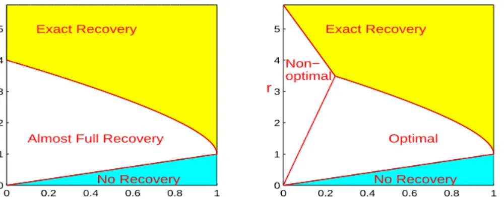
Al-so, for many different Ω, there is a common three-phase diagram in the two-dimensional phase space quantifying the signal sparsity and signal strength. In the first phase, it is possible to recover all signals. In the second phase, it is possible to recover most of the signals, but not all of them. In the third phase, successful variable selection is impossible. UPS partitions the phase space in the same way that the optimal procedures do, and recovers most of the signals as long as successful variable selection is possible.
The lasso and the subset selection are well-known approaches to variable selection. However, somewhat surprisingly, there are regions in the phase space where neither of them is rate optimal, even in very simple settings such asΩis tridiagonal, and when the tuning parameter is ideally set.
This part is joint work with Jiashun Jin, and has appeared in Annals of S-tatistics.
BIOGRAPHICAL SKETCH
Pengsheng Ji was born in 1981 in Shandong, China. He received B.S. in the Special Class of Mathematics and M.S. in statistics at Nankai University.
ACKNOWLEDGEMENTS
I wish to express my sincere gratitude to my advisors, Prof. Michael Nussbaum and Prof. Jiashun Jin. Their guidance, encouragement and friendship have giv-en me the greatest experigiv-ence.
Thanks to Prof. Jim Booth and Prof. Martin Wells for being on my PhD committee. Their suggestions and advice have been a valuable contribution to my work.
Thanks to Professors Robert Strawderman, J.T. Gene Hwang, Harry Zhou, David Ruppert, John Bunge and Giles Hooker for their support and tremendous help during my years of PhD study.
Thanks to my friends and fellow students Zhigen Zhao, Yingxing Li, Michael Grabchak, Bret Hanlon, Vadim Zipunnikov, Haizhi Jeff Lin, Gongfu Zhou and others.
TABLE OF CONTENTS
Biographical Sketch . . . iii
Dedication . . . iv
Acknowledgements . . . v
Table of Contents . . . vi
List of Tables . . . viii
List of Figures . . . ix
1 Sharp Adaptive Nonparametric Hypothesis Testing for Sobolev Ellip-soids 1 1.1 Introduction and main result . . . 1
1.2 The Bayes-minimax problem for nonparametric testing . . . 9
1.3 Proof of Theorem 1 . . . 14
1.4 Proof of Theorem 2 . . . 17
1.5 Appendix . . . 25
1.5.1 Ideas on adaptive estimation . . . 25
1.5.2 Proofs for Section 1.2 . . . 27
Bibliography 34 2 Sharp Asymptotics for Risk Bounds in Nonparametric Testing with Uncertainty in Error Distributions 37 2.1 Introduction . . . 37
2.2 The lower bound . . . 40
2.3 Attainment . . . 41 2.4 Proofs . . . 42 2.4.1 Proof of Lemma 2.4.1 . . . 46 2.4.2 Proof of Lemma 2.4.2 . . . 47 2.4.3 Proof of Lemma 2.4.3 . . . 49 Bibliography 52 3 UPS Delivers Optimal Phase Diagram in High Dimensional Variable Selection 53 3.1 Introduction . . . 53
3.1.1 Screen and Clean . . . 54
3.1.2 UPS . . . 55
3.1.3 Sparse signal model and universal lower bound . . . 58
3.1.4 Random design, connection to Stein’s normal means model 60 3.1.5 Optimality of the UPS . . . 61
3.1.6 Phase diagram for high dimensional variable selection . . 62
3.1.7 Non-optimal region for the lasso . . . 64
3.1.8 Non-optimal region for the subset selection . . . 67
3.1.10 Contents . . . 70
3.2 UPS and upper bound for the Hamming distance . . . 71
3.2.1 The Sure Screening property of theU-step . . . 73
3.2.2 The SAS property of theU-step . . . 74
3.2.3 Reduction to many small-size regression problems . . . . 75
3.2.4 P-step . . . 77
3.2.5 Upper bound . . . 78
3.2.6 Tuning parameters of the UPS . . . 79
3.2.7 Discussions . . . 80
3.3 A refinement for moderately large p . . . 81
3.4 Understanding the lasso and the subset selection . . . 83
3.4.1 Understanding the lasso . . . 84
3.4.2 Understanding subset selection . . . 89
3.5 Simulations . . . 92 3.6 Proofs . . . 97 3.6.1 Proof of Theorem 1.1 . . . 97 3.6.2 Proof of Lemma 2.1 . . . 100 3.6.3 Proof of Lemma 2.2 . . . 101 3.6.4 Proof of Lemma 2.3 . . . 102 3.6.5 Proof of Theorem 2.1 . . . 105 3.6.6 Proof of Lemma 2.4 . . . 116 3.6.7 Proof of Theorem 2.2 . . . 121 3.6.8 Proof of Lemma 3.1 . . . 122 3.6.9 Proof of Lemma 4.1 . . . 123 3.6.10 Proof of Lemma 4.2 . . . 125 3.6.11 Proof of Lemma 4.3 . . . 127 3.6.12 Proof of Lemma 4.4 . . . 128 Bibliography 135
LIST OF TABLES
3.1 The values of p2 log(p)p−[θ−(1−ϑ)]/2for different pand(θ, ϑ). . . 82 3.2 Hamming errors (Experiment 1). UPS needs weaker signals for
exact recovery. . . 93 3.3 Ratios between Hamming errors and pp (Experiment 2a-2c).
Bold: UPS. Plain: lasso. . . 94 3.4 Left: Ratios between the Hamming errors by the UPS and that
by the lasso (Experiment 4a). Right: Ratios between the Ham-ming errors by the UPS for the random design model and that for Stein’s normal means model (Experiment 4b). . . 96
LIST OF FIGURES
3.1 Left: Phase diagram. In the yellow region, the UPS recovers all signals with high probability. In the white region, it is possible (i.e., UPS) to recover almost all signals, but impossible to recover all of them. In the cyan region, successful variable selection is impossible. Right: partition of the phase space by the lasso for the tridiagonal model (3.1.11)-(3.1.12) (a = 0.4). The lasso is rate non-optimal in the Non-optimal region. The Region of Exact Re-covery by the lasso is substantially smaller than that displayed on the left. . . 64 3.2 Left: a re-display of the left panel of Fig 3.1. Right: partition of
the phase space by the subset selection in the tridiagonal model (3.1.11)-(3.1.12) (a= 0.4). The subset selection is not rate optimal in the Non-optimal region. The Exact Recovery region by the subset selection is substantially smaller than that of the optimal procedure, displayed on the left. . . 68 3.3 Partition of regions as in Lemma 3.4.1 (left) and in Lemma 3.4.3
(right). . . 89 3.4 Experiment 3a. x-axis: q. y-axis: Hamming error. Left to right:
ϑ=0.2,0.5,0.65. . . 94 3.5 Experiment 3b. x-axis: q. y-axis: Hamming error. Left: ϑ = 0.5.
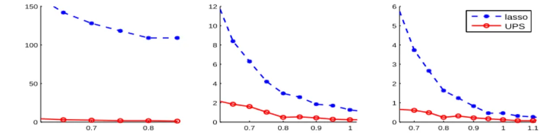
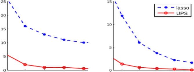
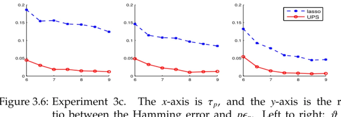
Right: ϑ= 0.65. . . 95 3.6 Experiment 3c. The x-axis is τp, and the y-axis is the ratio
CHAPTER 1
SHARP ADAPTIVE NONPARAMETRIC HYPOTHESIS TESTING FOR SOBOLEV ELLIPSOIDS
1.1
Introduction and main result
Consider the Gaussian white noise model in sequence space, where observa-tions are
Yj = fj+n−1/2ξj, j=1,2, ..., (1.1.1)
with unknown, nonrandom signal f = (fj)∞j=1, and noise variables ξj which are
i.i.d. N(0,1). It can also be written in the form of the stochastic differential equation
dY(t)= f(t)dt+n−1/2dW(t), t∈[0,1],
whereWis a standard Wiener process on[0,1], given an orthonormal basis. The asymptotic equivalence to nonparametric regression and density estimation has been established by Brown and Low (1996), and Nussbaum (1996).
We intend to test the null hypothesis of “no signal” against nonparametric alternatives described as follows. For someβ > 0and M > 0, let Σ(β,M)be the set of sequences Σ(β,M)={f = (fj)∞j=1 : ∞ X j=1 j2βfj2 ≤ M};
this might be called a Sobolev type ellipsoid with smoothness parameterβand size parameter M. Consider further the complement of an open ball in the se-quence spacel2: ifkfk22 =
P∞
j=1 f2j is the squared norm then
Hereρ1/2 is the radius of the open ball; by an abuse of language we callρitself
the “radius”. We study the hypothesis testing problem
H0 : f = 0 against Ha: f ∈Σ(β,M)∩Bρ.
Assuming thatn→ ∞, implying that the noise sizen−1/2tends to zero, we expect
that for a fixed radius ρ, consistent α-testing in that setting is possible. More precisely, there exist α-tests with type II error tending to zero uniformly over the nonparametric alternative f ∈ Σ(β,M)∩Bρ. If now the radiusρ = ρn tends
to zero asn→ ∞, the problem becomes more difficult and ifρn →0too quickly,
all α-tests will have the trivial asymptotic (worst case) power α. According to fundamental results of Ingster (1982, 1984), there is a critical rate forρn, the
so-calledseparation rate
ρn n−4β/(4β+1) (1.1.2)
at which the transition in the power behaviour occurs. More precisely, consider a (possibly randomized)α-testφnin the model (1.1.1) with respect toH0 : f = 0,
that is, a test fulfillingEn,0φn ≤ αwhereEn,f (·)denotes expectation in the model
(1.1.1). For givenφn, we define the worst case type II error over the alternative
f ∈Σ(β,M)∩Bρ as Ψ(φn, ρ, β,M) := sup f∈Σ(β,M)∩Bρ 1−En,fφn .
The search for a bestα-test in this sense leads to the minimax type II error
πn(α, ρ, β,M) := inf
φn:En,0φn≤α
Ψ(φn, ρ, β,M).
An α-test which attains theinf above for a givenn is minimax with respect to type II error. Ingster’s separation rate result can now be formulated as follows: ifρn n−4β/(4β+1)and0< α < 1then
0<lim
n
πn(α, ρn, β,M)and lim
Moreover, ifρn n−4β/(4β+1) then πn(α, ρn, β,M) → 0, and ifρn n−4β/(4β+1) then
πn(α, ρn, β,M)→ 1−α.
These minimax rates in nonparametric testing, presented here in the sim-plest case of an l2-setting, have been extended in two ways. Firstly, Ermakov
(1990) found the exact asymptotics of the minimax type II errorπn(α, ρ, β,M)
(e-quivalently, of the maximin power) at the separation rate. The shape of that result and its derivation from an underlying Bayes-minimax theorem on ellip-soids exhibit an analogy to the Pinsker constant in nonparametric estimation. Secondly, Spokoiny (1996) considered the adaptive version of the minimax non-parametric testing problem, where both β and M are unknown, and showed that the rate at which ρn → 0 has to be slowed by a log logn-factor if
nontriv-ial asymptotic power is to be achieved. Thus an “adaptive minimax rate” was specified, analogous to Ingster’s nonadaptive separation rate (1.1.2), where the additionallog logn-factor is interpreted as a penalty for adaptation. However a corresponding sharp adaptive type II error asymptotics in the sense of Ermakov (1990) has not been obtained.
It is noteworthy that in nonparametric estimation over f ∈ Σ(β,M)with l2
-loss (as opposed to testing), where the risk asymptotics is given by the Pinsker constant, there is a multitude of results showing that adaptation is possible with neither a penalty in the rate nor in the constant, cf. Efromovich and Pinsker (1984), Golubev (1987, 1992), Tsybakov (2009). The present paper deals with the question of whether the sharp risk asymptotics for testing in the sense of Ermakov (1990) can be reproduced in an adaptive setting, in the context of a possible rate penalty for adaptation.
testing in the nonadaptive setting. Let Φ be the distribution function of the standard normal, and for α ∈ (0,1) let zα be the upper α-quantile, such that
Φ(zα)=1−α. Writean bn(orbn an) iffbn= o(an), andan∼ bnifflimnan/bn= 1.
Proposition 1. (Ermakov, 1990) Supposeα ∈ (0,1),and that the radius ρn tends to zero at the separation rate, more precisely
ρn ∼c·n−4β/(4β+1), for some constantc>0.
(i) For any sequence of testsφnsatisfyingEn,0φn≤ α+o(1),we have the following lower bound Ψ(φn, ρn, β,M)≥ Φ(zα− p A(c, β,M)/2)+o(1)asn→ ∞, where A(c, β,M)= A0(β)M−1/(2β)c2+1/(2β) andA0(β)is Ermakov’s constant
A0(β)=
2(2β+1)
(4β+1)1+1/(2β). (1.1.3)
(ii) For givenβandM >0there exists a sequence of testsφnsatisfyingEn,0φn ≤ α+o(1) such that
Ψ(φn, ρn, β,M)≤ Φ(zα−
p
A(c, β,M)/2)+o(1).
This gives the sharp asymptotics for the minimax type II error at the separa-tion rate, analogous to the Pinsker constant for nonparametric estimasepara-tion. The optimal test attaining the bound of (ii) above, as given by Ermakov (1990), de-pends onβandM. As regards adaptivity in both of these unknown parameters, a test can not depend on them and the following result is known.
Proposition 2. (Spokoiny, 1996). LetT be a subset of(0,∞)×(0,∞)such that there existM >0,β2 > β1 >0and
T ⊇ {(β,M) :β1 ≤β≤ β2}.
(i) Iftn (log logn)1/2andρn ∼c·(n/tn)−4β/(4β+1), then for any constantc> 0and any adaptive testφnsatisfyingEn,0φn ≤α+o(1), we have
sup
(β,M)∈T
Ψ(φn, ρn, β,M)≥ 1−α+o(1).
(ii) For anyβ∗> 1/2
and0< M1≤ M2, let
T ={(β,M) : 1/2< β≤β∗,M1 ≤ M≤ M2}.
Then there exist a constant c1 = c1(β∗,M1,M2) and an adaptive test φn satisfying
En,0φn =o(1),such that, if
ρn ∼c1 n (log logn)1/2 !−4β/(4β+1) (1.1.4) then sup (β,M)∈T Ψ(φn, ρn, β,M)=o(1). (1.1.5)
Here the criterion to evaluate a test sequence has changed, to include the worst case type II error over a whole range of β,M. Hence the critical ra-dius rate (1.1.4) has to be interpreted as an adaptive separation rate. It differs by a factor (log logn)2β/(4β+1) from the nonadaptive separation rate (1.1.2); this factor is an example of the well-known phenomenon of a penalty for adapta-tion. Furthermore, as noted in Spokoiny (1996), a degenerate behaviour oc-curs here, in that both error probabilities at the critical rate tend to zero. Thus any sequenceφn of tests fulfilling (1.1.5) should be seen asadaptive rate optimal,
comparable to rate optimal tests in the nonadaptive case (that is, tests fulfilling limnΨ(φn, ρn, β,M) < 1−αat ρn given by (1.1.2)). In Ingster and Suslina (2003),
chap. 7, the worst case adaptive error (1.1.5) is further analyzed, with a view to a sharp asymptotics, but the results are not conclusive with regard discriminating between different adaptive rate optimal sequences of tests.
In this paper we address the question of whether an exact type II error asymptotics in the sense of Ermakov(1990) is possible in an adaptive setting. In our approachβis kept fixed and known, while we aim for adaptation over the ellipsoid size M. First, we present a negative result for adaptation at Ingster’s separation rate.
Theorem 1. Supposec > 0, 0 < M1 < M2 < ∞andρn ∼ c·n−4β/(4β+1). Then there is no adaptive testφnsatisfyingEn,0φn≤ α+o(1),such that
Ψn(φn, ρn, β,Mi)≤Φ(zα−
p
A(c, β,Mi)/2)+o(1),
fori= 1,2.
This result states sharp adaptation even just for M at the separation rate is impossible, and the adaptation for even justMis not trivial as some might think. Instead, we enlarge the radius slightly and examine how the minimax error approaches zero. To be specific, we replace the constantc in ρn ∼ c·n−4β/(4β+1)
by a sequence cn tending to infinity slowly. In that case the minimax type II
error bound of Proposition 1, namely Φ(zα − pA(c, β,M)/2) will tend to zero.
To this error probability we apply a log-asymptotics as in moderate and large deviation theory and show that in this sense, adaptation to Ermakov´s constant is possible.
cn·n−4β/(4β+1), there exists a testφnnot depending onMsuch that
En,0φn ≤ α+o(1), and for allM >0,
lim n 1 c2n+1/(2β) logΨ(φn, ρn, β,M)≤ − A0(β)M−1/(2β) 4
However now, since the optimality criterion has been changed, a formal ar-gument is needed that noα-test can be better in the sense of the log-asymptotics for the error of second kind. Such a result is implied by Theorem 3 in Ermakov (2008), where the nondaptive sharp asymptotics was studied in a setting where ρn = cn·n−4β/(4β+1) withcn → ∞, hence error probabilities tending to zero. Since
the nonadaptive minimax lower risk bound for fixedc is based on a Gaussian limit argument, the case ofcn → ∞(sufficiently slowly) should be treated with
the methodology of moderate deviations.
Theorem 3. Under the same assumptions as in the last theorem, ifρn =cn·n−4β/(4β+1), then for any testφn(possibly depending on M) satisfyingEn,0φn ≤α+o(1), we have
lim n 1 c2n+1/(2β) logΨ(φn, ρn, β,M)≥ − A0(β)M−1/(2β) 4 .
This result is implied by Theorem 3 in Ermakov (2008), and hence the proof is omitted.
We have a few remarks to address the relation to the literature.
1.) Ermakov (2008) also shows that, for nonadaptive testing, these asymp-totics of moderate deviation probabilities are valid in a sharper sense, i.e., there
are testsφn depending onMsuch that Ψ(φn, ρn, β,M)=(1+o(1))·Φ zα− q A0M−1/(2β)c2+1 /(2β) n /2 ! .
This is in the same spirit of the Cramer type of moderate deviation, as discussed for the central limit theorem by Chen et al. (2011), chap. 11. The question whether this sharper asymptotics can be replicated in the adaptive setting is open.
2.) Ingster(1993a, 1993b, 1993c, 1998) discussed the “detection” problem for `p
ball using the sum of the type I error and the maximum type II error. The conditions for which the sum of is bounded away from 0 and 1 are given. But no sharp or adaptive asymptotics is obtained.
3.) Golubev(1987) studied the adaptive estimation withβfixed, but incorpo-rates local aspects (twofold, both local with respect tox∈[0,1]and smoothness class) to construct the optimal test. In the current paper, we do not use the local aspects.
4.) In the literature, the testing problem considered here has sometimes been connected with the estimation problem of the quadratic functionalQ(f) = P∞
i=1 fj2, Ibragimov and Hasminskii(1980), Bickel and Ritov(1988) found that
when the unknown function is sufficiently smooth, quadratic functionals can be estimated with parametric √nrate, otherwise the rate is slower. More pre-cisely, the minimax rate with the parameter spaceΣ(β,M)isn−rwith an exponent r = 4β4+β1 < 12 when 0 < β < 1/4, but when β ≥ 1/4, the minimax rate becomes
n−1/2. Efromovich(1994) showed that at the point β = 1/4 the optimal adap-tive rate isn−1/2c
n wherecn → ∞slower than any power function of n, and for
β > 1/4, the optimal adaptive rate isn−1/2. Efromovich and Low(1996) showed
than the nonadaptive rate by a logarithmic factor. See Tsybakov (1998) for more discussion of the adaptive rates and of the boundary effects. Klemela (2006) found sharp adaptive estimators for the irregular caseβ <1/4. That is, first, the constantKβ,M is found such that
lim n→∞infQˆ sup (β,M)∈B Kβ,M(nlog √ n)−r−p sup f∈Σ(β,M) |Qˆ−Q(f)|p =1,
where B= [β1, β2]×[M1,M2], β2 < 1/4and p≥ 1. Second, the estimators which
do not depend on(β,M)and achieve the infimum are obtained.
The rest of the paper is organized as follows. In Section 2, we show that the minimax quadratic test is asymptotically minimax over all tests, and provide the idea of the proofs in Sections 3, 4 and 5. Finally, in the appendix, we re-cap the ideas for adaptive estimation of Golubev (1992) to help the readers to understand the idea of adaptive testing.
1.2
The Bayes-minimax problem for nonparametric testing
The purpose of this expository section is to elucidate the analogy between the Pinsker constant for L2-estimation over ellipsoids and the constant found by
Ermakov (1990) for nonparametric testing over ellipsoids with an L2-ball
re-moved. We draw on the backgound explanation given in Ingster and Suslina (2003), sec. 4.1, but we focus specifically on the fact that very similar Bayes-minimax problems are at the root of the estimation and testing variants. For the theory underlying the Pinsker constant cf. Belitser and Levit (1995), Nussbaum (1999), Tsybakov (2009).
1, . . . ,n; we will thus assume f ∈ Rn
and understand the sets Σ(β,M) and Bρ accordingly, i.e. they refer only to the firstncoefficents of f. Byk·kandh·,·iwe
denote euclidean norm and inner product in Rn. Since most expressions will
depend on n, for this discussion we shall often suppress dependence on n in the notation. Assume that the radius ρ tends to zero at the critical rate, that is ρ n−4β/(4β+1). Let R+n = [0,∞)n; for a certain d ∈ Rn+, consider a quadratic
statistic of the form T˜ = nPn
j=1djY2j. Under H0, we have En,0T˜ = P n
j=1dj and
Var0,nT˜ = 2kdk2. Since we will work with the normalized test statistic, obtained
by centering and dividing by the standard deviation, it is obvious that we need only consider coefficientsdfulfillingkdk2 = 1. Accordingly define, for such co-efficientsd, the statistic
T = √1 2 ˜ T − n X j=1 dj . (1.2.6)
UnderH0, we now haveE0T =0andVar0T = 1.We will consider quadratic tests
ψd =1{T >zα}. (1.2.7)
A further condition ondis imposed by requiringd ∈ D, a set which is defined
for a given sequenceδ= logn−1 as D ={d∈Rn+:kdk2 =1and sup j d2j ≤ δ nρ}. (1.2.8)
For any test, we are interested in the worst case type II error under the constraint f ∈ Σ(β,M) ∩ Bρ. A monotonicity argument shows that for every ψd, this is
attained whenkfk2is minimal, i.e. atkfk2 =ρ. It follows that for quadratic tests
ψd, we may replace the restriction f ∈Bρby f ∈B0ρwhere
B0ρ ={f ∈Rn :ρ≤ kfk2≤ 2ρ}. For f ∈Rnwe set f2 :=f2 j n j=1. Ford∈ Dandg∈R n
+define the functional L(d,g)= √n
2
Lemma 1.2.1. (a) UnderH0, we haveT N(0,1)uniformly overd∈ D.
(b) The statisticT given by (1.2.6) fulfills
T −L(d, f2) N(0,1)
uniformly overd ∈ Dand f ∈B0ρ.
(c) Suppose f is random such that fj ∼ N
0, σ2
j
for a certainσ∈Rn. Then the statistic
T given by (1.2.6) fulfills
T −L(d, σ2) N(0,1)
uniformly overd ∈ Dandσ∈B0
ρ.
Denote the expectation under the model of (c) by Eσ∗. The lemma implies that for uniformly overd∈ Dand f ∈ {0} ∪Σ(β,M)∩B0ρ
Ef(1−ψd)= Φ(zα−L(d, f2))+o(1) (1.2.9) = E∗f(1−ψd)+o(1). (1.2.10)
In particular, all quadratic tests ψd with d ∈ D are aymptotic α-tests
un-der H0 : f = 0. To characterize the worst case error under the alternative
Ha : f ∈Σ(β,M)∩Bρ, we use (1.2.9) and the strict monotonicity ofΦand look for
a saddlepoint of the functionalL(d, f2).
Lemma 1.2.2. Fornlarge enough, there exists a saddlepointd0 ∈ D, f0 ∈Σ(β,M)∩B0ρ
of the functionalL(d, f2)such that
L(d, f02)≤ L(d0, f02)≤ L(d0, f2) for alld∈ Dand all f ∈Σ(β,M)∩B0ρ.
The normal distribution on the signal f postulated in (c) will be interpreted as a prior distribution. The next result shows that the Bayesian tests in this con-text are quadratic testsψd, and in particular, if theσ2is taken at the saddlepoint
(σ2 0 = f
2
0) thend ∈ D, i.e. it fulfills the infinitesimality conditiond 2
j ≤δ/nρ.
Lemma 1.2.3. (a) For anyσ2 ∈
Rn+, the Neyman-Pearsonα-test for simple hypotheses
H0 : Yj ∼ N(0,n−1), j=1, . . . ,n
Ha∗: Yj ∼ N(0, σ2j +n−1), j=1, . . . ,n
is equivalent to a quadratic test pof formψd = 1{T > t}whereT = Pnj=1djY2j,d ∈Rn+,
kdk =1. (b) Ifσ2 = f2
0 then the pertainingdis inDfornlarge enough, andt →zα.
Part (b) implies that
inf φ:E0φ≤αE ∗ f0(1−φ)= inf d∈DE ∗ f0(1−ψd)+o(1). (1.2.11)
We are now ready to present the essence of the argument underlying the result of Ermakov (1990). Recall that πn(α, ρ, β,M)denotes the minimax type II error
over allα-tests. Denote the value of L(d, f2)at the saddlepoint
L0 := L(d0, f02)=sup d∈D inf f∈Σ(β,M)∩B0 ρ Ln(d, f2)= inf f∈Σ(β,M)∩B0 ρ sup d∈D Ln(d, f2). (1.2.12) We begin with an α0 > α
such that asymptotic α-tests are α0
enough. Then πn(α0, ρ, β,M)= inf φ:E0φ≤α0 sup f∈Σ(β,M)∩Bρ Ef (1−φ)≤ inf d∈Df∈Σ(supβ,M)∩B ρ Ef(1−ψd) (1.2.13) = inf d∈Df∈Σ(supβ,M)∩B0 ρ Ef(1−ψd) = inf d∈Df∈Σ(supβ,M)∩B0 ρ Φ(zα−Ln(d, f2))+o(1)[relation (1.2.9)] = Φ(zα−Ln(d0, f02))+o(1)[monotonicity ofΦand (1.2.12)] = inf d∈DE ∗ f0(1−ψd)+o(1)[relation (1.2.10)] = inf φ:E0φ≤α E∗f 0(1−φ)+o(1)[relation (1.2.11)].
The main term of the last expression is the Bayes risk for a prior distribution fj ∼ N(0, f0j2)in the original modelYj ∼ N
fj,n−1
. Since f0 ∈Σ(β,M)∩B0ρand is extremal there, it fulfills
n X j=1 f02jj2β = M, n X j=1 f02j = ρ
(see the precise description of the saddlepoint (d0, f0) in Lemma 1.5.1 below).
It can therefore be shown that (as in the original Pinsker [1980] result) that this prior distribution asymptotically concentrates on every set of the formΣ(β,M(1+ ε))∩B0ρ(1−ε)forε >0. A standard reasoning by truncation shows that in this case, for a certain probability measureGstrictly concentrated onΣ(β,M(1+ε))∩B0
ρ(1−ε) inf φ:E0φ≤αE ∗ f0(1−φ)≤φinf :E0φ≤α Z Ef(1−φ)dG(f)+o(1).
However, by the relation between Bayes and minimax risk
inf φ:E0φ≤α
Z
Ef(1−φ)dG(f)≤πn(α, ρ(1−ε), β,M(1+ε)). (1.2.14)
Summarizing (1.2.13)-(1.2.14) we have obtained for everyε >0
Below in Lemma 8, it is shown that ifρ= c·n−4β/(4β+1), wherecis constant, then L(d0, f02)∼
p
A0M−1/(2β)c2+1/(2β)/2.
Since the right side is continuous inMandc, the result of Proposition 1 follows.
1.3
Proof of Theorem 1
For brevity we writeAi = A(c, β,Mi),i= 1,2in this section. Assume there exists
a testφn not depending onisuch that
En,0φn ≤α+o(1), (1.3.15) sup f∈Σ(β,Mi)∩Bρ En,f(1−φn)≤ Φ(zα− p Ai/2)+o(1), (1.3.16)
fori = 1or2. LetGn,Mi be the Gaussian prior for f with fj ∼ N(0, σ
∗2
j )
indepen-dently, where
σ∗2
j (Mi)=(λ−µj2β)+, j=1,2, . . .
and whereλandµare determined by X
j2βσ∗2j = Mi and
X σ∗2
j =ρ.
It can be shown thatGn,Mi asymptotically concentrates onΣ(β,Mi). Then
sup
f∈Σ(β,Mi)∩Bρ
En,f(1−φn)≥(1+o(1))·
Z
En,f(1−φn)Gn,Mi(d f). (1.3.17)
p Recall Yj = fj +n−1/2ξj. Let the joint distributions of (Yj)∞0 under the priors
Gn,0,Gn,M1 andGn,M2 beQ0,n,Q1,nandQ2,n, respectively, i.e.,
Q0,n :Yj ∼ N(0,n−1), j=1,2, . . .
Q1,n :Yj ∼ N(0,n
−1+σ∗2
j (M1)), j= 1,2, . . .
Therefore,
EQ0,nφn= En,0φn,
EQi,n(1−φn)=
Z
En,f(1−φn)Gn,Mi(d f), i= 1,2.
Combining these with (1.3.16) and (1.3.17) gives
EQ0,nφn≤ α+o(1), (1.3.18)
EQi,n(1−φn)≤Φ(zα−
p
Ai/2)+o(1), i= 1,2. (1.3.19)
The likelihood ratio ofQi,nagainstQ0,nis
dQi,n dQ0,n =exp −1 2 X j Y2j n−1+σ∗2 j (Mi) − Y 2 j n−1 ·Y j n−1 n−1+σ∗2 j (Mi) 1/2 =exp 1 2 X j n2σ∗2j (Mi) 1+nσ∗2 j (Mi) Y2j ·Y j n−1 n−1+σ∗2 j (Mi) 1/2 .
Therefore, by the factorization theorem, it is seen that the bivariate vector
Tn= X j n2σ∗2j (M1)(Y2j −n −1) (1+nσ∗2 j (M1)) q 2n2P kσ∗4k (M1) ,X n 2σ∗2 j (M2)(Y 2 j −n −1) (1+nσ∗2 j (M2)) q 2n2P kσ∗4k (M2)
is a sufficient statistic for the family of distributions {Q0,n,Q1,n,Q2,n}. Write the
induced family for Tn as {QT0,n,QT1,n,QT2,n} and take the conditional expectation
φ∗
n(Tn) = EQi,n(φn|Tn). By sufficiency (Bahadur´s theorem, cf. Lehmann and
Ro-mano, 2005, chap. 11), the (possibly randomized) testφ∗
n(Tn)for{QT0,n,QT1,n,QT2,n} is as good asφn, i.e., EQT0,nφ ∗ n= En,0φn ≤α+o(1), (1.3.20) EQT i,n(1−φ ∗ n)=EQ1,nφn ≤Φ(zα− p Ai/2)+o(1), i=1,2. (1.3.21)
Lemma 1.3.1. Under {Q0,n,Q1,n,Q2,n}, the law of the statistic Tn converges in total variation toN(0,Σ),N(µ1,Σ)andN(µ2,Σ)respectively, where
µ1 =( p A1/2,r p A1/2)0, µ2 =(r p A2/2, p A2/2)0, Σ = 1 r r 1 , r= M1 M2 !1/(4β) · 4β+1−M1/M2 4β . (1.3.22)
Then by the weak compactness theorem (c.f. Lehmann and Romano, 2005, Appendix), there exists a testφ∗
and a subsequenceφ∗ nk such that φ ∗ nk converges weakly toφ∗ . Thus EQT 0,nφ ∗ ≤α, EQT i,n(1−φ ∗ )≤ Φ(zα− pAi/2), i=1,2.
By the Neyman-Pearson lemma and some direct calculations, the right hand side of the previous inequality is the type II error of the uniformly most pow-erful test for N(0,Σ)against N(µi,Σ), for i = 1,2, respectively. Therefore,φ∗ is a
uniformly most powerful test forN(0,Σ)against{N(µ1,Σ),N(µ2,Σ)}.
On the other hand , note thatr in Lemma 1.3.1 is monotone increasing with respect to M1/M2, and then 0 < r < 1 for M2 > M1 > 0. Thus, µ1, µ2 and the
origin are not on the same line. For i = 1,2 respectively, the log-likelihood ratio for N(µi,Σ) against N(0,Σ) is T0−1µi = Ti · Ai. Then by the necessity part
of the Neyman-Pearson lemma, (cf. Lehmann and Romano, 2005, chap. 3), the uniformly most powerful test for N(0,Σ)against N(µi,Σ)has the form of 1{Ti >
most powerful test for N(0,Σ)against{N(µ1,Σ),N(µ2,Σ)}. By this contradiction,
Theorem 1 is proved.
Proof of Lemma1.3.1. For simplicity, we only show the result for the first coordi-nate ofTn. The proof can be extended toTn naturally. UnderQ0,n, the
character-istic function ofn(Y
2 j−1/n) √ 2 ∼ N(0,1)isg(t)=exp(−t 2/2). Noteg(t)= 1−1 2t 2+o(t2), as
t→0andR |g(t)|<∞. The density ofTn,1can be written as
pn(x)= 1 2π Z e−itxYg σ∗2 j (M1)·t (1+nσ∗2j (M1)) q P kσ∗4k (M1) ,
where, by the central limit theorem and Levy’s continuity theorem, the inte-grand converges toe−itxexp{−t2/2}. By splitting the integral into two parts and using dominated convergence, it can be shown that the integral converges to
1 2π Z e−itxe−t2/2dt = e −x2/2 √ 2π.
Then an application of Scheff´e’s theorem (c.f. van der Vaart, 1998) establishes convergence in total variation. The correlationrcan be calculated directly.
1.4
Proof of Theorem 2
ChooseN˜ andγn =o(1)such that
γ1/2β n ·n 2/(4β+1) N˜ c−1/(2β) n ·n 2/(4β+1), (1.4.23)
e.g.γn =c−1n /2,N˜ = c −1/(3β) n ·n2/(4β+1). Define M0 = M0(f)= ˜ N X j=1 j2βfj2+γn, N = N(M0)= (4β+1)M0 ρ !1/(2β) , ˜ λ= λ(M˜ 0)= 2β+1 2β 1 M0(4β+1) !1/(2β) ρ(2β+1)/(2β), ˜ dj = d˜j(M0)=λ[1˜ −(j/N)2β]+,
which all depend on the unknown f. Define the oracle statistic
Tn∗ = n2P jd˜j(M0)Y2j −n P jd˜j(M0) q 2n2P jd˜2j(M0) ,
and the oracle testφ∗ n =1{T
∗
n > zα}. The following lemma holds; it is proved later.
Lemma 1.4.1. Under the assumptions of Theorem 2, the oracle testφ∗
nis an asymptotic α-test and lim n 1 c2n+1/(2β) logΨ(φ∗n, ρn, β,M)≤ − A0(β)M−1/(2β) 4 Define ˆ M= ˜ N X j=1 (Y2j −1/n)j2β+γn
and introduce the statistic
Tn= n2P ˜ dj( ˆM)Y2j −n P ˜ dj( ˆM) q 2n2P ˜ d2j( ˆM) and also the test
φn = 1{Tn >zα}.
Lemma 1.4.2. Under the assumptions of Theorem 2, we have ˆ M M0(f) −1=op(1), uniformly for f ∈Σ(β,M)∩Bρ. Now rewrite Tn = X j ˜ dj( ˆM) q P ˜ d2 j( ˆM) · Y 2 j −1/n √ 2n−2 ,
whered˜j( ˆM)=λ(1˜ −(j/N( ˆM))2β)+. Sinceλ˜ in the last display can be canceled, for
simplicity we writed˜j( ˆM) =(1−(j/N( ˆM))2β)+from now on in this section. First,
sinceN( ˆM)≥ N(γn), we have X ˜ d2j( ˆM)= X 1− j N( ˆM) !2β 2 + ∼ N( ˆM) Z 1 0 (1−t2β)2+dt = N( ˆM)K(β). Therefore, Tn= (1+o(1)) X d˜j( ˆM) q N( ˆM)K(β) · Y 2 j −1/n √ 2n−2 . By Lemma 1.4.2, Tn =(1+o(1)) X j ˜ dj( ˆM) p N(M0(f))K(β) · Y 2 j −1/n √ 2n−2 .
At this point, makeMˆ independent ofY2j by sample splitting. Setn=τn+(1−τ)n,
where τis close to 1 but fixed, andn1 = τn,n2 = (1−τ)n. Assume two sets of
observations
Y1j = fj+n−1
/2
1 ξ1j, j=1,2, . . . (1.4.24)
Use{Y2j}to obtain M, and now replaceˆ Tn by Tns =(1+o(1)) X j ˜ d( ˆM) p N(M0(f))K(β) · Y 2 1j−n −1 √ 2n−1 .
Denote the difference of coefficients by∆j = d˜j( ˆM)−d˜j(M0(f)). Note the largest
difference is obtained at j≈ min{N( ˆM),N(M0(f))}. Then
|∆j| ≤ |Mˆ −M0(f)|
γn
uniformly for all j. Note inT1 there are at mostC2c −1/(2β) n n2/(4β+1) nonzero coeffi-cients. Then Tns =(1+o(1)) C2c−n1/(2β)n2/(4β+1) X j=1 ˜ dj(M0(f)) p N(M0(f))K(β) ηj+rn whereηj = Y12j−n−1 1 √ 2n−1 1 , and rn = C2c −1/(2β) n n2/(4β+1) X j=1 ∆jηj p N(M0(f))K(β) .
Under H0, the r.v.´s ηj are independent of Mˆ and Eηj = 0, Var(ηj) = 1. Thus
Var(rn)= Er2n = EE(r2n|{Y2j})and
E(rn2|{Y2j})= E C2c −1/(2β) n n2/(4β+1) X j=1 ∆2 j N(M0(f))K(β) ≤ |Mˆ − M0(f)| 2 γ2+1/(2β) n . Therefore, by the result forVar( ˆM)in the proof of Lemma 1.4.2,
Var(rn)≤ E|Mˆ −M0(f)|2 γ2+1/(2β) n = Var( ˆM) γ2+1/(2β) n ≤ 2K(β) ˜N 4β+1 n2γ2+1/(2β) n + 4 ˜N2βM nγ2+1/(2β) n ,
where the last two terms converge to0by the first inequality in (1.4.23). Hence, underH0, the r.v.´sTnandTnsconverge toN(0,1)in law.
Next, we considerTnorTnsunder the alternative. The worst case type II error
is determined by the following quantity
Ln = n √ 2 f∈Σ(infβ,M)∩Bρ PN˜ j=1 fj2d˜j( ˆM) P ˜ dj( ˆM) 1/2.
First, sinceN( ˆM)≥γn cn 1/(2β) ·n2/(4β+1) → ∞, ˜ d2j = ˜ N X j=1 1−(j/N)2β2 + =(1+o(1))N Z 1 0 (1−t2β)2dt =(1+o(1))N· 8β 2 (2β+1)(4β+1). (1.4.26) Second, consider ˜ N X j=1 fj2d˜j( ˆM)= ˜ N X j=1 f2j(1−(j/N) 2β )+. Note ˜ N X j=1 fj2 = ∞ X j=1 f2j − ∞ X j=N˜+1 fj2 ≥ρ−N˜−2βM =ρ 1− M ρN˜2β ! =ρ(1+o(1)), (1.4.27)
where the last step is refers to the second inequality of (1.4.23). On the other hand, sinceN˜ N andN( ˆM)=[(4β+1) ˆMρ−1]1/(2β),
N X j=1 f2j(j/N)2β+ ˜ N X j=N+1 fj2 ≤ ˜ N X j=1 fj2(j/N)2β ≤N−2βM0(f) =ρ(1+4β)−1. (1.4.28) Combining (1.4.30)-(1.4.32) gives ˜ N X j=1 fj2d˜j ≥(1+o(1)) ˜λρ· 4β 4β+1.
Combining this with (1.4.29) gives nPN˜ j=1 fj2d˜j (2P ˜ d2j)1/2 ≥(1+o(1)) n √ 2 s 2(2β+1) 4β+1 ρ 2/N ≥(1+o(1)) s (2β+1)c2n+1/(2β) (4β+1)1+1/(2β)(M+γ n)1/(2β) ≥(1+o(1)) r 1 2A0(β)c 2+1/(2β) n M−1/(2β) Theorem 2 is proved.
Proof of Lemma 1.4.1. Rewrite
Tn∗= X j ˜ dj(M0(f)) q P ˜ d2 j(M0(f)) · Y 2 j −1/n √ 2n−2 .
UnderH0, we have f = 0, andM0(f)= γn. Since
X [1−(j/N)2β]2+∼ N· Z 1 0 (1−t2β)2dt = K(β)·(γn/cn)1/2βn2/(4β+1), then ˜ dj(M0(f)) q P ˜ d2j(M0(f)) ≤ 1 p K(β)·(γn/cn)1/2βn2/(4β+1) =o(1), uniformly for all j. It can be shown thatT∗
n converges toN(0,1)in law.
By similar arguments, the worst type II error is(1+o(1))Φ(z−Ln)where
Ln = inf f∈Σ(β,M)∩Bρ nP f2 jd˜j (2P ˜ d2 j)1/2 .
Note d˜j = d˜j(M0(f)) depending on f. By the second inequality of (1.4.23), we
haveN˜ N(M0(f))andd˜j =0,for j≥ N,˜
Ln= n √ 2 f∈Σinf(M)∩Bρ PN˜ j=1 fj2d˜j (P ˜ d2 j)1/2 .
First, sinceN(M0(f))≥ γ n cn 1/(2β) ·n2/(4β+1) → ∞uniformly for f ∈Σ(β,M)∩Bρ, ˜ d2j =λ˜2 ˜ N X j=1 1−(j/N)2β2 + =(1+o(1)) ˜λ2N Z 1 0 (1−t2β)2dt =(1+o(1)) ˜λ2N· 8β 2 (2β+1)(4β+1), (1.4.29) uniformly for f ∈Σ(β,M)∩Bρ. Second, consider
˜ N X j=1 fj2d˜j =λ˜ ˜ N X j=1 fj2(1−(j/N)2β)+=λ˜ ˜ N X j fj2− N X j fj2(j/N)2β+ ˜ N X j=N+1 fj2 . (1.4.30) Note ˜ N X j=1 fj2 = ∞ X j=1 f2j − ∞ X j=N˜+1 fj2 ≥ρ−N˜−2βM =ρ 1− M ρN˜2β ! =ρ(1+o(1)), (1.4.31)
where the last step is due to the second inequality of (1.4.23). On the other hand, sinceN˜ N andN = [ρ−1(4β+1)M 0(f)]1/(2β), N X j=1 f2j(j/N) 2β+ ˜ N X j=N+1 fj2 ≤ ˜ N X j=1 fj2(j/N) 2β ≤N−2βM0(f) =ρ(1+4β)−1 (1.4.32) Combining (1.4.30)-(1.4.32) gives ˜ N X j=1 f2jd˜j ≥(1+o(1)) ˜λρ· 4β 4β+1
uniformly for f ∈Σ(β,M)∩Bρ. Combining this with (1.4.29) gives nPN˜ j=1 fj2d˜j (2P ˜ d2j)1/2 ≥(1+o(1)) n √ 2 s 2(2β+1) 4β+1 ρ 2/N ≥(1+o(1)) s (2β+1)c2n+1/(2β) (4β+1)1+1/(2β)(M+γ n)1/(2β) ≥(1+o(1)) s (2β+1)c2n+1/(2β) (4β+1)1+1/(2β)M1/(2β),
uniformly for f ∈Σ(β,M)∩Bρ. Therefore, Ln ≥(1+o(1)) r 1 2A0(β)c 2+1/(2β) n M−1/(2β),
and the result follows.
Proof of Lemma 1.4.2. Since
Var( ˆM)= ˜ N X j=1 2 n2 + 4fj2 n j 4β ≤(1+o(1))2K(β) ˜N 4β+1 n2 + 4 ˜N2βM n , by the first inequality of (1.4.23),
Var( ˆM) γ2
n
=o(1)
uniformly for f ∈Σ∩Vρ. Combining withEMˆ = M0(f)and using Chebyshev’s
inequality give Mˆ −M0(f) γn =op(1), and then ˆ M M0(f) −1 ≤ Mˆ −M0(f) γn =op(1), uniformly for f ∈Σ∩Vρ.
1.5
Appendix
1.5.1
Ideas on adaptive estimation
Consider the estimation problem for the Gaussian sequence model
Yj = fj +n −1/2ξ
j
withP
j2βfj2 ≤ M. It is known, for given M, the optimal filter is(1−µjβ)+, where µis determined by 1 n X jβ(1−µjβ)+= µM. Since µ∼ β·n −1 M(β+1)(2β+1) !β/(2β+1) , the optimal truncation is of the ordern1/(2β+1).
Choosen1/(2β+1/2) N˜ n1/(2β+1)and1γ n N˜2β+1/2/n, and define M0,f = ˜ N X j=1 j2βf2j +γn. Define N = N(M0,f) = α· n1/(2β+1)M 1/(2β+1)
0,f , where αis a constant to be chosen.
Define
dj = d(j/N)=
1−(j/N)β +. Consider the oracle estimator(djYj)∞1. Its risk is
X (1−dj)2f2j + 1 n X d2j = ˜ N X j=1 (1−dj)2f2j + X j>N˜ (1−dj)2f2j + 1 n X d2j :=A1+A2+A3.
First, A1 ≤sup j≤N˜ (1−dj)2j−2βM0,f ≤ N−2βM0,f = α−2βn−2β/(2β+1)(M+γn)1/(2β+1) Second,A2 =Pj>N˜ fj2≤ N˜ −2βM= o(n−2β/(2β+1)). Third, A3= N n 1 N X (1−(j/N)β)2+ ≤ αn−2β/(2β+1)(M+γn)1/(2β+1) Z ∞ 0 (1−tβ)2+dt = αn−2β/(2β+1)(M+γ n)1/(2β+1)· 2β2 (β+1)(2β+1)
These results hold uniformly over f. Combine these and choose α = (β+1)(2β+1)
β
1/(2β+1)
, and we have the supremum risk of the oracle estimator over f is at most c(m)·n−2β/(2β+1)M1/(2β+1), where c(m)= β β+1 !2β/(2β+1) ·(1+2β)1/(2β+1) is the Pinsker constant.
Let Mˆn =P ˜ Nn j=1 j 2βfˆ2 j +γn, where fˆ 2 j =y 2 j −n −1. Then E( ˆM)= ˜ Nn X j=1 j2βfj2 = M0,f ≤ M+γn and Var( ˆM)= ˜ N X j=1 j4βVar(Y2j) = ˜ N X j=1 j4βn−2(2+4n fj2) =2n−2 ˜ N X j=1 j4β+4n−1 ˜ N X j=1 j4βfj2 = J1+J2,
where the first term J1 =2n−2N˜4β+1· 1 ˜ N ˜ N X j=1 j/N˜4β ∼ 2n−2N˜4β+1·K =o(1) sinceN˜ =o(n1/(2β+1/2)), and the second term
J2≤ 4n−1N˜2β ˜ N X j=1 j2βfj2 =4n −1 ˜ N2βM0,f .4K Mn−2N˜4β+1· n ˜ N2β+1 = o(J1)
uniformly for f ∈ Σ(β,M)since N˜ n1/(2β+1). Combining these gives Var( ˆM) =
o(1)uniformly for f ∈Σ(β,M). Recallingγn N˜2β+1/2/ngives
Var ˆ M− M0,f γn ∼ 2Kn−2N˜4β+1 γ2 n =o(1), and then ˆ M M0,f −1 ≤ ˆ M−M0,f γn =op(1) (1.5.33) uniformly.
The last result is crucial for the next step, i.e. showing that the difference between oracle estimatordjYj
∞
1 and the estimator
d( j
N( ˆM))Yj
∞
1 is negligible. Re
call that N = N(M0,f); now (1.5.33) is used to replace M0,f by estimate M. Theˆ
remainder of the proof consists of showing
EX d(j/N(M0,f))−d(j/N( ˆM))
2
Y2j = o(n
−2β/(2β+1)).
1.5.2
Proofs for Section 1.2
Proof of Lemma 1.2.1. (a) Under the null hypothesis we have Y2j = n−1ξ2j, hence T = P dj ξ2 j −1
/√2. Then it follows from (1.2.8) and nρ → ∞ that the CLT
infinitesimality condition
sup
j
holds uniformly overd ∈ D, proving the assertion. (b) SinceY2j = fj2+2n−1/2f jξj+n−1ξ2j, we have T = √1 2 X dj n fj2+2n 1/2 fjξj+ ξ2 j −1 , (1.5.34) T −L(d, f)= √1 2 X dj 2n1/2fjξj+ ξ2 j −1 . (1.5.35)
An easy calculation gives
VarfT =
1 2
X
d2j4n fj2+2= 1+2nXd2jfj2
where in view of (1.2.8) we have for f ∈B0
ρ nXd2jf 2 j ≤δρ −1X fj2 ≤2δ= o(1).
Consequently,VarfT → 1uniformly. Now the CLT infinitesimality condition on
the sum (1.5.35) amounts to
sup
j
d2jn fj2+1= o(1). (1.5.36)
For f ∈ B0
ρ we have fj2≤ 2ρ, hence in view of (1.2.8)
d2j n f2j +1 ≤d2j(2nρ+1)≤2δ
for n sufficiently large. Hence (1.5.36) is fulfilled uniformly over d ∈ D and
f ∈B0
ρ, and the claim follows.
(c) Set fj ∼ N(0, σ2j); then in view of (1.5.34)
T −L(d, σ)= √1 2 X dj 2n1/2fjξj+ ξ2 j −1 + √n 2 X dj fj2−σ2j . (1.5.37)
An easy calculation gives
VarfT = 1 2 X d2j 4nσ2 j +2 +nXd2j =1+nXd2j2σ2j +σ4j
where in view of (1.2.8) we have forσ∈B0ρ nXd2jσ 2 j ≤δρ −1Xσ2 j ≤ 2δ=o(1), nXd2jσ 4 j ≤2ρn X d2jσ 2 j ≤4ρδ= o(1).
Consequently,VarfT → 1uniformly. Now the infinitesimality condition on the
sum (1.5.37) amounts to sup j d2j 1+nσ2j +nσ4j =o(1). (1.5.38) Forσ∈ B0ρ we haveσ2 j ≤2ρ, hence in view of (1.2.8) d2j 1+nσ2j +nσ 4 j ≤ d2j 1+nρ+nρ2≤ 3δ
for n sufficiently large. Hence (1.5.38) is fulfilled uniformly over d ∈ D and
σ∈B0ρ, and the claim follows.
Proof of Lemma 1.2.2 . LetD˜ be defined asDin (1.2.8) but with conditionkdk2 =1 replaced bykdk2 ≤ 1. Then, since L(d, f)is linear ind, for everyd˜∈D˜ there is a d∈ Dsuch thatL( ˜d, f2)≤ L(d, f2)for every f. Hence it suffices to prove the claim forDreplaced by the compact convex setD˜. The restriction f ∈Σ(β,M)∩B0ρis equivalent to f2being in the set
n g∈Rn+:Xgjj2β ≤ M, ρ≤ X gj ≤ 2ρ o (1.5.39)
which is convex and compact (and nonempty for large enoughnsince ρ → 0). The functional L is bilinear in d and f2; the standard minimax theorem now
Lemma 1.5.1. Fornlarge enough, the saddlepointd0, f0of Lemma 1.2.2 is given by d0 = f02 f 2 0 , f02,j = λ−µj2β +, j=1, . . . ,n
whereλ, µare the unique positive solutions of the equations n X j=1 j2βλ−µj2β += M, n X j=1 λ−µj2β +=ρ. (1.5.40)
The value ofLat the saddlepoint is
L0 =L(d0, f0)= n √ 2 f 2 0 . (1.5.41)
Proof. Ignore initially the restriction supjd2
j ≤ δ/nρ and consider maximizing
L(d, f2)indfor given f. Under the sole restrictionkdk =1, by Cauchy-Schwartz the solution is found as
d(f)= f 2 f2 . It remains to minimizeL(d(f), f) = n f 2 / √
2under the restrictions on f2.
Set-ting gj = fj2, one has to minimizekgk on the convex set (1.5.39). This is solved
using Lagrange multipliersλ, µ.
To show that the solutiond0fulfills the restrictionsupjd2j ≤δ/nρ, we note that
f02,j = λ−µj2β += λ 1−µλ−1j2β + ≤λ; (1.5.42)
below (cf. (1.5.49), Lemma 1.5.2) it is shown that λ n−1−1/(4β+1) and n f 2 0 Ln,0 1. This implies nρd2 0,n,j = nρ·O n2λ2, n3ρλ2 n·n−4β/(4β+1)·n−2/(4β+1) =n−1/(4β+1; (1.5.43) thus forδ = logn−1
Proof of Lemma 1.2.3. The log-likelihood ratio is log n−1n/2 σ2 j +n−1 n/2 exp −1 2 n X j=1 Y2j σ2 j +n −1 − Y2j n−1 = 1 2 n X j=1 nY2j nσ2 j nσ2 j +1 − n 2 n X j=1 lognσ2j+1.
This shows (a) by settingd = d/˜ d˜ ford˜j = nσ2 j nσ2j+1. Now forσ 2 j = f 2 0j we have, as λ n−1−1/(4β+1), n f02j = nλ1−λ−1µj2β + ≤nλ n·n −1−1/(4β+1) = n−1/(4β+1)= o(1), henced˜j ∼n f02juniformly over j=1, . . . ,n. This implies
d˜ ∼ n f 2 0 nand dj = ˜ dj d˜ f02j uniformly in j≤n. The proof ofnρd2
0,n,j ≤ δnow exactly follows (1.5.42), (1.5.43)
(CHECK). The convergencet→ zαnow is a consequence of Lemma 1.2.1 (a). Lemma 1.5.2. Supposeρ= c·n−4β/(4β+1),cconstant. Then the saddlepoint valueL0of (1.2.12) fulfills
L0= L(d0, f02)∼
p
A0M−1/(2β)c2+1/(2β)/2.
Proof. The proof of Lemma 1.5.1 shows thatL(d0, f02)is also the saddlepoint
val-ue under the weaker restrictions kdk2 ≤ 1, f ∈ Σ(β,M) ∩ Bρ. Let us sketch a derivation of the asymptotics by a renormalization technique. Suppose that dj = h1/2d(h j), j ≤ n where h is a bandwidth parameter tending to 0, and the
continuous functiond: [0,∞)→[0,∞)satisfies Z ∞
0
d2(x)dx≤ 1. (1.5.44)
Consider another continuous functionσ : [0,∞)→ [0,∞)satisfying Z ∞ 0 x2βσ2(x)dx≤1 and Z ∞ 0 σ2(x)dx≥1 (1.5.45)
and setσ2
j = Mh
2β+1σ2(h j), j ≤ n. Chooseh = (ρ/M)1/(2β). The coefficient vector
d= dj n j=1satisfies kdk2 = h n X j=1 d(h j)→ Z ∞ 0 d(x)dx ≤1. Identifying f2 ∈ Rn+ with (σ2 j) n
j=1, the restriction f ∈ Σ(β,M) is asymptotically
satisfied since ∞ X j=1 j2βσ2j = Mh ∞ X j=1 (jh)2βσ2(jh)→ M Z ∞ 0 x2βσ2(x)dx ≤ M, h→0.
The restriction f ∈ Bρ is also asymptotically satisfied since
∞ X j=1 σ2 j = Mh 2β+1 ∞ X j=1 σ2(jh)= ρh ∞ X j=1 σ2(jh)∼ρ Z ∞ 0 σ2(x)dx≥ρ. Therefore, n √ 2 n X j=1 djσ2j = n √ 2Mh 2β+1/2 h ∞ X j=1 d(jh)σ2(jh) ∼ c 1+1/(4β)M−1/(4β) √ 2 Z ∞ 0 d(x)σ2 (x)dx.
The saddle point problem (1.2.12) for eachnis thus asymptotically expressed in terms of a fixed continuous problem with constraints (1.5.44) and (1.5.45). There is unique positive solution(λ∗, µ∗)
for the equations (cp. Golubev, 1982), Z ∞ 0 x2β(λ−µx2β)dx=1, (1.5.46) Z ∞ 0 (λ−µx2β)dx=1. (1.5.47)
Let k·k2 and h·,·i2 denote norm and scalar product in L2(R+). Then the saddle
point(d∗, σ∗2)is given by d∗ = σ ∗2 σ∗2 2 , σ∗2 (x)= (λ∗−µ∗x2β)+. (1.5.48)
Then the value of the game is sup din (1.5.44) inf σin (1.5.45) D d, σ2E 2 =σin (1.5.45)inf sup din (1.5.44) D d, σ2E 2 =D d∗, σ∗2E 2= σ ∗2 2 = p A0(β),
where the sup is taken for d satisfying (1.5.44), the inf is taken for σ satisfy-ing (1.5.45), and A0(β) is Ermakov’s constant in (1.1.3). The continuous
sad-dlepoint problem arises naturally in a continuous Gaussian white noise setting and a parameter space described by the continuous Fourier transformation, e.g. a Sobolev class of functions on the whole real line (cf. Golubev 1982, 1987).
The above argument provides the guideline for a more rigourous proof, based on calculating the sharp asymptotics of λ and µ directly from (1.5.40). The rough order ofλcan be found as follows. By equating f02 = σ∗2j , we find
λ−µj2β + = Mh 2β+1σ∗2(h j), =λ1−(µ/λ)1/2β j2β + we findλh2β+1,h (µ/λ)1/2βand thus
λh2β+1 (ρ)(2β+1)/(2β) n−1−1/(4β+1. (1.5.49)
Remark 1.5.1. The paper of Ermakov (1990), when calculating the asymptotics ofλ, µ in (1.5.40) and ofA= 2L20(in a more general framework where P
ajfj2 ≤ P0,
P
bjfj2 ≥
ρ), contains an error for λ. Here is the correction using the notations therein. Let
aj = L j2γ, bj = M j2ν, where γ > ν ≥ 0, L and M are positive constants, and set
=n−1/2. Then as →0we have that
λ∼ (2γ+2ν+1) 2(γ−ν) L P0(4γ+1) !2(4νγ+−1ν) 1 M !2(4γγ+−1ν) ρ(4ν+ 1)2(2(γ+γν−)ν+)1 ,
µ∼ (4ν+1)ρλ
P0(4γ+1)
, A∼ −4ρλ4γ−4ν
4γ+1 .
Bibliography
[1] BELITSER, E., LEVIT, B. (1995). On minimax filtering on ellipsoids. Math.
Meth. Statist.4259-273
[2] BROWN, L. D., and LOW, M. G. (1996). Asymptotic equivalence of
nonpara-metric regression and white noise.Ann. Statist.242384–2398.
[3] CHEN, L. H. Y., GOLDSTEIN, L. and SHAO, Q.-M. (2011).Normal Approxi-mation by Stein’s method. Springer, Heidelberg.
[4] EFROMOVICH, S and PINSKER, M.S. (1984). A learning algorithm for
non-parametric filtering.Automat. Remote Control111434–1440.
[5] ERMAKOV, M. S. (1990). Minimax detection of a signal in a white gaussian
noise,Theory Probab. Appl35667–679.
[6] ERMAKOV, M. S. (2008). Nonparametric hypothesis testing for small type I and type II error probabilities,Probl. Inform. Transmission44no. 2, 54–74.
[7] GOLUBEV, G. K. (1987). Adaptive asymptotically minimax estimates of
s-mooth signals.Probl. Inform. Transmission2357–67.
[8] GOLUBEV, G. K. (1992). Nonparametric estimation of smooth probability
densities in L2.2844–54.
[9] GOLUBEV, G. K. and NUSSBAUM, M. (1990). A risk bound in Sobolev class regression,Ann. Statist.18758–778.
[10] INGSTER, Yu. I. (1982). Minimax nonparametric detection of signals in white Gaussian noise.Probl. Inform. Transmission 18, no. 2, p. 61
[11] INGSTER, Y. I. (1993a). Asymptotically minimax hypothesis testing for non-parametric alternatives. I.Mathematical Methods of Statistics285C114.
[12] INGSTER, Y. I. (1993b). Asymptotically minimax hypothesis testing for
non-parametric alternatives. II.Mathematical Methods of Statistics2171C189.
[13] INGSTER, Y. I. (1993c). Asymptotically minimax hypothesis testing for
non-parametric alternatives, III.Mathematical Methods of Statistics2249C268.
[14] INGSTER, Y. I. (1998). Minimax detection of a signal for`n-balls. Mathemati-cal Methods of Statistics7401C428.
[15] INGSTER, Yu. I., SUSLINA, I. A. (2003).Nonparametric Goodness-of-fit
Test-ing under Gaussian models.Lecture Notes in Statistics, 169. Springer-Verlag,
New York.
[16] INGSTER, Yu. I and SUSLINA, I. A. (2004). Nonparametric hypothesis test-ing for small type I errors. I.Math. Methods Statist.13no. 4, 409–459.
[17] INGSTER, Yu. I and SUSLINA, I. A. (2005). Nonparametric hypothesis test-ing for small type I errors. II.Math. Methods Statist.14no. 1, 28–52.
[18] LEHMANN, E. L. and ROMANO, J. P. (2005).Testing Statistical Hypotheses.
Springer, NY.
[19] NUSSBAUM, M. (1996). Asymptotic equivalence of density estimation and Gaussian white noise.Ann. Statist.242399–2430.
[20] NUSSBAUM, M. (1999). Minimax risk: Pinsker bound. In: Encyclopedia of
Statistical Sciences, Update Volume 3, 451-460 (S. Kotz, Ed.). Wiley, New
York.
[21] ROHDE, A. (2008). Adaptive goodness-of-fit tests based on signed ranks.
Ann. Statist.361346–1374.
[22] SPOKOINY, V. G. (1996) Adaptive hypothesis testing using wavelets.Ann.
Statist.242477–2498.
[23] TSYBAKOV, A. B. (2009). Introduction to Nonparametric Estimation. Springer, NY
CHAPTER 2
SHARP ASYMPTOTICS FOR RISK BOUNDS IN NONPARAMETRIC TESTING WITH UNCERTAINTY IN ERROR DISTRIBUTIONS
2.1
Introduction
We are interested in the hypothesis testing problems for nonparametric regres-sion. Consider the observations
yi = f(xi)+ξi, xi ∈[0,1], i= 1,2, ...,n, (2.1.1)
where {ξi,n} are independent random variables with zero expectation, and the
function f is to be tested. The nonradom points xi are assumed to be generated
by a densitygon[0,1]such that Z xi,n
0
g(t)dt = i/n.
We define some smoothness class of functions. LetL2 = L2(0,1)be the Hilbert
space of square integrable functions on[0,1]and letk · kdenote the usual norm
therein. Let, for naturalm and f ∈ L2, Dmf denote the derivative of orderm in
the distributional sense and let
W(m)={f ∈L2 : Dmf ∈L2}
be the corresponding Sobolev space on the unit interval. The Sobolev class of ordermand radius Mis defined by
W(m,M)={f ∈W(m) : kDmfk2 ≤ M}
for givenmand M >0. The periodic Sobolev class is
e
Let{ψj, j=1, ...}be a orthonormal basis such that e W(m,M)={f : f = ∞ X j=1 fjψj, ∞ X j=1 ajf2j ≤ M}, whereaj ∼ (πj)2m.
Define the complement of an open ball inL2
Bρ = {f ∈L2: kfk2 ≥ ρ}.
We consider the hypothesis testing problem of
H0 : f = 0 against Ha : f ∈W(m,M)∩Bρ.
If the radius ρn tends to zero too quickly, all tests will have tivial asymptotic
power; if it tends to zero too slowly, there exists an α-test such that the type II error tends to zero and consistent testing is possible. Brown and Low [3] established the asymptotic equivalence of the regression model to the Gaussian white noise model,
dY = f(t)dt+σdW(t),
where W(t) is the Browning motion. In the more general framework of the Gaus-sian white noise model, Ingser [7, 6] established the separation rate of
ρn n
−4m/(4m+1)
for Sobolev ellipsoids, for which the asymptotic type II error is bounded away from 0 and 1. More precisely, define the minimax type II error as
πn(α, ρn,m,M) := inf φn:En,0φn≤α sup f∈W(m,M)∩Bρ (1−En,fφn). Ifρn n−4β/(4β+1)then 0<lim n πn(α, ρn,m,M) and lim n πn(α, ρn, β,M)< 1−α.
Ermakov [4] found the exact asymptotics of the minimax type II error at the separation rate. More precisely, if
ρn ∼c·n−4β/(4β+1),
for somec> 0, then
πn(α, ρn,m,M)= Φ(zα−
p
A(c, β,M)/2)+o(1) asn→ ∞,
whereA(c, β,M)=A0(β)M−1/(2β)c2+1/(2β)and A0(β)is the Ermakov’s constant
A0(β)=
2(2β+1)
(4β+1)1+1/(2β). (2.1.2)
In the present paper we consider the sharp asymptotics of the minimax type II error for the model (2.1.1) with uncertain error distributions. This notation of uncertainty is related with robustness, e.g. [2]. As shown below, the mod-el giving meaning meaningful results here is one the nonidentical distributed errors. The distributions of ξi will still vary in a small neighborhood of some
(unknown) central measureQ0, but will in general be different.
In contrast, it is noteworthy that substantial attention has been devoted to asymptotically minimax estimation for integrated mean square error. For the Sobolev class of problems, it has been possible to improve the results on best obtainable rates of convergence by find the exact asymptotic value of the mini-max risk in the class of all estimators. The key original result is due to Pinkser [9] for a filtering problem over ellipsoids in Hilbert space. Nussbaum [8] and Speckman [10] considered the regression model with Gaussian errors. Golubev and Nussbaum [5] extended the sharp asymptotics to non-Guassian regression for which the error distributions are from a neighborhood of some central mea-sure, and may be nonidentical.
2.2
The lower bound
Our main interest is the testing problem for regression with uncertain error dis-tributions. We adopt the same formulation for the uncertain error distributions as in [5].
Let, for distributionsQ0and Q,
H(Q0,Q)= Z (dQ0)1/2−(dQ)1/2 2 !1/2
be the Hellinger distance. Consider a sequenceτn such that
τn →0, τnn1/2→ ∞asn→ ∞.
Introduce the set of probability measures on the real line:
QHn = {Q;H(Q0,Q)≤ τn,EQξ=0}. (2.2.3)
The central measureQ0has zero expectation, second momentσ2and fulfills the
following regularity condition: IfQ0t denotes the shifted measureQ0t = Q0(·+t),
then
H(Q0t,Q0)= O(t) ast →0. (2.2.4)
We assumeα∈(0,1).
Theorem 2.2.1. Assume in the model (2.1.1), ξi are independent with distribution
Q ∈ QnH, where the central measure Q0 has zero expectation, second moment σ2 and fulfills(2.2.4).
(i) Ifδ2 = c·n−4m/(4m+1), then, for any testφ
nsatisfyingE0φn =α+o(1),
lim
n
where
A= A(M,m,c, σ)= A0(m)c
2+1/(2m)
σ4M1/(2m) , (2.2.5) andA0(m)= (1+2π4m)(1+1+2m)1/(2m) is Ermakov’s constant.
(ii) Ifδ2 = o(n−4m/(4m+1)). Then for any testφ
n satisfying E0φn = α+o(1), we have
limnβ(φn)=1−α.
2.3
Attainment
A complete argument for attainment is beyond the scope of the paper, but we provide theoretical backings for our claim that the lower bounds are indeed attainable.
Consider first the regression model (2.1.1) withg≡1and normal noise with varianceσ2. It is known that the error bound in Theorem 2.2.1 is attained by a
quadratic statistic given in the frequency domain, [4]. In the time domain 2.1.1, this corresponds to a quadratic statistic given by some linear spline smoothing procedure.
In the nonnormal case, when the noise in 2.1.1 is uncorrelated with zero expectation and varianceσ2, the risk behavior of the quadratic statistics
men-tioned above remains valid. Actually, the proofs show that the error II error depends only on the first two moments of the noise. The noise distribution model in Theorem 2.2.1 ensures that Varξ ∼ σ2. Indeed, for Q ∈ QH
have |EQx2−σ2|2= | Z x2d(Q−Q0)|2 (2.3.6) ≤ Z x4((dQ)1/2+(dQ0)1/2)2 ! H2(Q0,Q) (2.3.7) ≤ 4cH2(Q0,Q)=o(1). (2.3.8)
Thus it obvious that the bound of Theorem 2.2.1 is attainable for g ≡ 1 and knownMandσ2.
For adaptation for unknown M, we conjecture the plug-in-type method de-veloped in the last chapter still works, and some sharp asymptotics can be es-tablished by an adaptive smoother. But we leave this study to the future.
2.4
Proofs
Consider the Sobolev spaceWe2mwith boundary conditions on[0,1]:
e
W2m ={f ∈W2m; (Dkf)(0)= (Dk)f(1)= 0,k= 0, ...,m−1}.
It is a Hilbert subspace ofWm
2 with respect to the norm(kfk
2 +kDmfk2)1/2. We
will make use of the results on the spectral theory of differential operators; see, e.g., Agmon [1].
There exists a basisϕj, j = 1,2, ..., in We2m such that, if (·,·) denotes the inner product inL2(0,1),
(ϕi, ϕj)=δi j, (2.4.9)
(Dmϕi,D mϕ
where
0< λ1 < λ2 <· · ·
and the asymptotics of the eigenvaluesλj is given by
λj ∼(πj)2m, j→ ∞.
The boundary conditions ensure that, when the functions ϕj are continued by
zero outside [0,1], the functions belong to the Sobolev space of ordermon any interval containing [0,1]. Furthermore, this property allows the construction of another orthogonal system inWe2mwhich is obtained by a change of scale. Fix a natural numberq. Later we will letqtend to infinity withn. Define functions
ϕjkq=q1/2ϕj(qx−k+1), k=1, ...,q, j=1,2....
Each functionϕjkqis inWe2m, has support[(k−1)q−1,kq−1]and
(ϕjkq, ϕikq)=δi j (2.4.11)
(Dmϕikq,Dmϕjkq)=q2mλjδi j. (2.4.12)
Furthermore, fix a naturalsand defineW(q,s,M)as the intersection of the linear span ofϕjkq, j=1, ...,s, k= 1, ...,q, withWe2m(M). From (2.4.12), we obtain that for
f ∈W(q,s,M), kDmfk2 = s X j=1 q X k=1 q2mλj(ϕjkq, f)2
and obviously W(q,s,p) is nonempty. Restricting f to this set, we reduce the problem to the one of testing the local Fourier coefficients fjkq = (ϕjkq, f). The
indicesqand n will frequently be dropped from the notation in the sequel.
By restricting f to the subsetW(q,s,M), we achieve that the observationsyi
have a structure yi = s X j=1 ϕjk(xi)fjk+ξi, i= 1,2, ...,n, (2.4.13)
where k is uniquely defined by i ∈ F(k) := {i;xi ∈ q−1(k −1,k]}. This may be
constructed as a collection of q linear regression models, each accounting for observations in the intervalq−1(k−1,k]and havingsparameters. The parameters
fjksatisfy s X j=1 q X k=1 q2mλjfjk2 ≤ M, and s X j=1 q X k=1 fjk2 ≥δ 2. Let δ2 = c·n−4m/(4m+1), λ=a·n−1/(4m+1), q=[b·n2/(4m+1)],
whereaandbdo not depend onnand will be selected later.
Introduce the column vectors, fork= 1,2, ...,q,
hk =n1/2(f1k, ..., fsk)0, (2.4.14) ¯ ϕi =n −1/2(ϕ 1k(xi), .., ϕsk(xi)) 0. (2.4.15)
Then the model (2.4.13) transforms to
yi =ϕ¯0ihk+ξi, i∈ F(k), (2.4.16)
fork= 1,2, ...,q. Now we will select the disturbance distributions inQH∩QML in
accordance with the method of least favorable parametric subfamilies. Consider a bounded functionψonRsuch that, ifuis the identity map inR,
Z
ψdQ0= 0,
Z
Sethk = λ1/2gk. Forg∈Rs, letQi(g)be the measure defined by
dQi(g)=(1+λ1/2ϕ¯0igψ)dQ0.
LetQ∗
i(g)be the shifted measure
Q∗i(g)(·)= Qi(g)(·+λ1/2ϕ¯0ig).
Lemma 2.4.1. Letτn be the sequence in the definitionQHn and lettn be such thattn →
∞, tn = o(τnn(1−r)/2) as n → ∞. Then for sufficiently large n, the set of measures
{Q∗i(g);kgk ≤tn,i∈ {1,2, ...,n}}is contained inQHn ∩Q M L. Define κ2 j = 1−(j/s)2m +, j= 1,2, ...
and introduce the prior distribution ongjk as independentN(0, κ2j), j = 1,2, ...,.
Letνkbe the product prior ongk. Obviouslyνk,k =1,2, ...,qare iid. The induced
product prior on all fjk, j=1,2, ...,q=1,2, ...,qwill be denoted byΠn.
Lemma 2.4.2. For givenc>0and a small numberτ >0, set
a= c(1+τ) K1 !(2m+1)/(2m) · K2 M(1−τ) !1/(2m) , (2.4.17) b= 1 s MK1(1−τ) cK2(1+τ) !1/(2m) , (2.4.18)
where K1 = 2m2m+1 and K2 = (2m+1)(4m2m +1). Then, for sufficiently large s, we have Πn(We(m,M)∩Bρ)→ 1asn→ ∞.
Consider the corresponding Bayesian testing problem
H0∗:yi ∼ Q0, iid.