Lower Bounds on Active Learning for Graphical Model Selection
Jonathan Scarlett and Volkan Cevher
Laboratory for Information and Inference Systems (LIONS) École Polytechnique Fédérale de Lausanne (EPFL)
Email: {jonathan.scarlett, volkan.cevher}@epfl.ch
Abstract
We consider the problem of estimating the underlying graph associated with a Markov random field, with the added twist that the decoding algorithm can iteratively choose which subsets of nodes to sample based on the previous samples, resulting in an active learning setting. Considering both Ising and Gaussian models, we pro-vide algorithm-independent lower bounds for high-probability recovery within the class of degree-bounded graphs. Our main results are minimax lower bounds for the active setting that match the best known lower bounds for the passive setting, which in turn are known to be tight in several cases of interest. Our analysis is based on Fano’s inequality, along with novel mutual information bounds for the active learning setting, and the application of restricted graph ensembles. While we con-sider ensembles that are similar or identical to those used in the passive setting, we re-quire different analysis techniques, with a key challenge being bounding a mutual informa-tion quantity associated with observed sub-sets of nodes, as opposed to full observations.
1
Introduction
Graphical models are a widely-used tool for providing compact representations of the conditional indepen-dence relations between random variables, and arise in areas such as image processing [1], statistical physics [2], computational biology [3], natural language pro-cessing [4], and social network analysis [5]. The prob-lem of graphical model selection consists of recovering
Appearing in Proceedings of the 20th International
Con-ference on Artificial Intelligence and Statistics (AISTATS) 2017, Fort Lauderdale, Florida, USA. JMLR: W&CP vol-ume 54. Copyright 2017 by the authors.
the graph structure given a number of independent samples from the underlying distribution. While this problem is NP-hard in general [6], there exist a vari-ety of methods guaranteeing exact recovery with high probability on restricted graph classes, with a partic-ularly common restriction being bounded degree. Several variations of graphical model selection prob-lems with active learning have appeared in the liter-ature. In this paper, we adopt the formulation given in [7], in which the recovery algorithm may adaptively choose which nodes to sample, based on the previous samples. The goal is to recover the underlying graph subject to a constraint on the total number of node observations. As discussed in [7], this variation is of interest in several applications; for example, in sen-sor networks one may be able to choose which sensen-sors to activate, rather than simultaneously activating ev-ery sensor at evev-ery time instant. Only upper bounds were provided in [7], and the problem of finding lower bounds was left as an open problem.
1.1 Contributions
In this paper, we complement the work of [7] by pro-viding algorithm-independent lower bounds on active learning for graphical model selection. Our main find-ings are summarized as follows:
1. For both Ising models and Gaussian models, we provide lower bounds that essentially match the best known lower bounds for the passive setting [8, 9], in terms of the minimax probability of er-ror with respect to the class of bounded-degree graphs. The passive learning bounds are known to be tight in several cases of interest, and our re-sults show that active learning does not help sig-nificantly in the minimax sense in such cases. 2. We provide a class of Gaussian graphical
mod-els where the average degree dictates the lower bounds as opposed to the maximal degree, and where we match upper bounds based on the aver-age degree in [7]. Hence, we identify a graph class
where the average degree is provably the funda-mental quantity dictating the fundafunda-mental lim-its. Moreover, we provide a class of Ising models where the maximal degree provably remains the key quantity dictating the performance, hence re-vealing that one cannot always improve the de-pendence from the maximal to the average degree. Our analysis uses a variation of Fano’s inequality for the active learning setting, along with novel mutual in-formation bounds proved using analogous techniques to those used in channel coding with noiseless feed-back [10]. We apply the resulting bound to a variety of restricted graph ensembles in which the graphs are difficult to distinguish from each other, with notable examples being (i) isolated edges that are difficult to detect; (ii) cliques with a single edge removed such that the removal is difficult to detect. While the ensembles that we use are similar or identical to those used in the passive setting, analyzing them in the active set-ting requires new techniques, particularly for bounding a mutual information quantity associated with partial observations instead of full observations.
1.2 Related Work
In the same way that feedback often provides little or no gain in the capacity for channel coding [10], it is often observed that active learning provides little or no gain in the information-theoretic sample complexity of inference and learning problems. For example, in the compressive sensing problem, it has been shown that the improvement amounts to at most a logarithmic factor [11]. For the group testing problem, under a broad range of scalings of the sparsity level, not even the constant factors improve [12, 13].
On the other hand, active learning is known to strictly improve the sample complexity in several cases of in-terest [14, 15]. Moreover, it should be noted that even when adaptivity does not help asymptotically in an information-theoretic sense, it can still help in the sense of leading to simpler and less computationally expensive algorithms, and also in improving the non-asymptotic performance [13, 15, 16].
Active learning for graphical model selection has been studied in several contexts [7, 17, 18], the most rele-vant to ours being that of Dasarathy et al. [7]. A general algorithm was proposed therein using abstract subroutines for neighborhood selection and neighbor-hood verification, and applications to the Gaussian setting revealed cases where the total number of node observations is improved fromO(dmaxplogp)toO((1+
dmax)plogp). Here dmax is the average of the
node-wise maximal degree, where the latter is defined as the highest degree among a node and all its neighbors.
This quantity can be significantly smaller than dmax,
in which case the improvement in the sample complex-ity is substantial.
Information-theoretic lower bounds for the passive set-ting were given in [8, 19–24] for the Ising model, and [9, 25, 26] for the Gaussian model. Let en be the sample complexity with respect to the number of p-dimensional observations. The best minimax lower bounds for degree-bounded graphs are summarized as follows for the Ising model [8]:
e n= Ω max logp λtanhλ, eλdlog(pd) λdeλ , dlog p d , (1) where pis the number of nodes,dis the maximal de-gree, and λ is the inverse temperature of the Ising model (see Section 2 for precise definitions). For the Gaussian model, the best known lower bounds for degree-bounded graphs are [9]
e n= Ω max logp τ2 , dlogpd log(1 +dτ) , (2) where τ corresponds to the smallest allowed off-diagonal magnitude in the normalized inverse covari-ance matrix (see Section 2 for details).
A wide range of polynomial-time algorithms have been proposed for the passive learning of graphical models; see [19, 20, 24, 27–32] for Ising models, and [20, 33–35] for Gaussian models. The best performance bounds among these algorithms match those of (1)–(2) in sev-eral cases of interest, though there are other cases where gaps remain, or where the results are difficult to compare due to the differences in the underlying assumptions (e.g., additional coherence assumptions). 1.3 Structure of the Paper
In Section 2, we formally define the Ising and Gaus-sian graphical models, and formulate the active learn-ing problem. Our main results are presented and dis-cussed in Section 3. The proofs are given in Section 4.1 (Fano’s inequality), Section 4.2 (Ising model), and Section 4.3 (Gaussian model). In Section 5, we dis-cuss the role of the average vs. maximal degree, and we conclude our work in Section 6.
2
Active Learning for Graphical
Model Selection
2.1 Preliminaries
We consider a collection of p random variables
(X1, . . . , Xp) whose joint distribution is encoded by
{1, . . . , p} and undirected edge set E. The elements ofV are referred to asnodes orvariables interchange-ably. We use the standard terminology that thedegree of a nodei∈V is the number of edges inEcontaining i, and that aclique is a fully-connected subset ofV of cardinality at least two.
We consider two classes of joint probability distribu-tions encoded by G, namely, Ising models and Gaus-sian models. These are described as follows.
Ising Model: In the ferromagnetic Ising model [36,37], each vertex is associated with a binary random variableXi∈ {−1,1}, and the corresponding joint
dis-tribution is described by the probability mass function PG(x) = 1 Z exp λ X (i,j)∈E xixj , (3)
whereZ is a normalizing constant called the partition function. Here λ >0 is a parameter to the distribu-tion, sometimes called the inverse temperature. In the context of Ising model selection, we writeGd as
Gd,λ to emphasize that the results depend on λ.
Al-though we let λbe a constant here, our lower bounds remain valid in the minimax sense when one considers the larger class in which the edges have differing pa-rameters{λij}in the range[λmin, λmax], provided that
λmin≤λ≤λmax.
Gaussian Model: In the Gaussian graphical model [37], each vertex is associated with a random variable Xi∈R, and the corresponding joint distribution is
(X1, . . . , Xp)∼N(0,Σ), (4)
where 0 is the vector of zeros, and Σ is a covari-ance matrix whose inverseΣ−1contains non-zeros only in the diagonal entries and the indices correspond-ing to pairs in E. By the Hammersley-Clifford the-orem [37], this implies the Markov property for the graph, namely, that a given node is conditionally in-dependent of the rest of the graph given its neighbors. The joint density function corresponding to (4) is de-noted by PG, overloading the notation used above for
the Ising model.
A typical restriction on the entries ofΘ = Σ−1is that
|Θij|
√
ΘiiΘjj
is lower bounded by some constant τ > 0
[7, 9]. We consider the simplest special case of this in which the lower bound always holds with equality:
Θij= 1 i=j ±τ (i, j)∈E 0 otherwise. (5)
We write Gd asGd,τ to emphasize that the results
de-pend on τ. Similarly to the Ising model, our lower
Decoder Choose Nodes
X
(i) GˆZ
(i+1)G
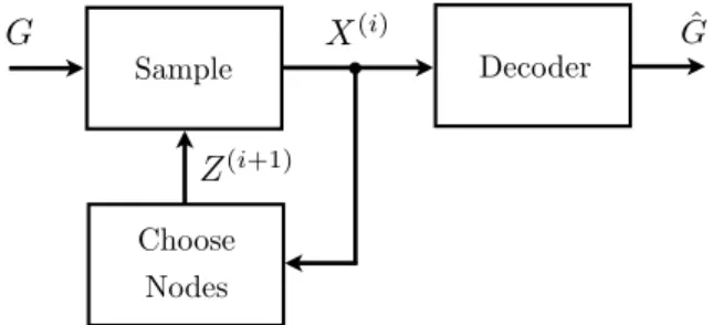
SampleFigure 1: Illustration of the active learning problem for graphical model selection.
bounds remain valid in the minimax case when we consider the larger class with √|Θij|
ΘiiΘjj
∈ [τmin, τmax]
withτmin≤τ ≤τmax.
2.2 Problem Statement
The problem of graphical model selection with active learning proceeds in rounds i= 1,2, . . ., as illustrated in Figure 1. In the i-th round, the algorithm selects a subset of V to observe, encoded by a binary vector Z(i) ∈ {0,1}p equaling one for observed nodes and
zero for non-observed nodes. The resultingsample (or observation) is a p-dimensional vectorX(i)such that:
• The joint distribution of the entries of X(i),
cor-responding to the entries whereZ(i) is one,
coin-cide with the corresponding joint distribution of the vector(X1, . . . , Xp)∼PG, with independence
between rounds;
• The values of the entries ofX(i), corresponding to the entries whereZ(i)is zero, are deterministically
given by∗, a symbol indicating that the node was not observed.
For convenience, we letN denote the maximum possi-ble number of active learning rounds (e.g., we can sim-ply setN =n), and use the convention that for values of ibeyond the actual (possibly random) final round, X(i) = (∗, . . . ,∗). Letting |Z(i)| denote the number
of entries where Z(i)is one, we refer toPN
i=1|Z(i)|as
thetotal number of node observationsused throughout the course of the algorithm, and we impose an upper bound on its maximum allowed value, denoted by n. Note that this differs from the quantity en in (1)–(2) by a factor ofp.
After the final round, the algorithm constructs an es-timate Gˆ ofG, and the error probability is given by
Pe(G) :=P[ ˆG6=G]. (6) We consider the classGdof degree-bounded graphs, in
are interested in bounds on the minimax (worst-case) error probability for graphs in this class:
Pe := max
G∈Gd
P[ ˆG6=G], (7) where the dependence on the total number of node samplesnis kept implicit. Note that when we consider the Gaussian setting, the maximum in (6) is not only over the graph G, but also implicitly over the signs (+1or −1) in the second case of (5).
We are interested in characterizing the sample com-plexity, meaning the required number of node obser-vations n needed in order to achievePe ≤δ for some
target error probabilityδ >0.
3
Main Results
In this section, we state and discuss our main results, namely, minimax lower bounds on the sample com-plexity for Gd. We note that the proofs are based
on graph ensembles in which the maximal degree and average degree are approximately equal; however, in Section 5, we discuss variations of these ensembles in which these two notions differ significantly.
3.1 Ising Model
Theorem 1. For Ising graphical models withλd≥1, in order to recover any graph in Gd,λ with probability
at least 1−δ, it is necessary that the total number of node observations,n, satisfies
n≥max ( 2plogp λtanhλ, eλdlog(pd) 2λdeλ , pdlog8pd 4 log 2 ) ×(1−δ−o(1)). (8)
Proof. See Section 4.2.
The second bound in (8) reveals that the sample com-plexity is very large when λd → ∞ at a rate that is not too slow, due to the exponential termeλd. On the
other hand, when λ =O 1
d
, the first bound gives a sample complexity ofΩ(d2plogp), sincetanhλ=O(λ)
as λ→0. Finally, in any case, the third bound gives n = Ω pdlogpd
. These observations coincide with those for the lower bounds on passive learning in [8] (see (1) with ne = np), suggesting that active learn-ing does not help much in the minimax sense forGd,λ.
Note that compared to [8], we lose a factor ofpin the second bound, but this factor is insignificant compared to eλd provided thatλdlogp.
3.2 Gaussian Model
Theorem 2. For Gaussian graphical models withd=
o(p), in order to recover any graph inGd,τ with
proba-bility at least1−δ, it is necessary that the total number of node observations, n, satisfies
n≥max ( 4plogp log 1 1−τ2 , 2pdlog p d log1 + (d+ 1)1−ττ2 ) ×(1−δ−o(1)). (9) Proof. See Section 4.3.
When τ = o(1), the first bound behaves as
Ω τ12plogp
, whereas when τ is a constant, the sec-ond bound behaves asΩ 1
logd·pdlog p d
. Both of these scaling laws are identical to the necessary conditions for passive learning in [9] (see (2) withne=np), again suggesting that active learning does not help much in the minimax sense forGd,τ.
While the above findings indicate that active learning does not help much in the minimax sense for Gd, we
discuss a more restricted class of graphs in Section 5 for which active learning helps when τ is a constant. Specifically, similarly to the upper bound in [7], the linear dependence on the maximal degreedin the sec-ond term of (9) is improved to the average degree.
4
Proofs of Main Results
4.1 Fano’s Inequality for Active Learning We first apply Fano’s inequality [10] along with a novel mutual information bound for active learning in graph-ical model selection. The proof bears some resem-blance to that of the converse bound for channel coding with noiseless feedback [10, Sec. 7.12].
For z ∈ {0,1}p, we let G(z) denote the subgraph of
G obtained by keeping only the nodes corresponding to entries where z equals one, and denote the result-ing joint distribution by PG(z). More generally, for
a joint distribution Q on prandom variables labeled
{1,· · ·, p}, we let Q(z) denote the joint marginal
dis-tribution corresponding to the entries where zis one. In the following lemma, we letGbe uniformly random on some subset of Gd, and define the average error
probability
Pe:=P[ ˆG6=G] =E[Pe(G)], (10)
where in contrast with (7), the probability is now ad-ditionally over G. Clearly any lower bound on the sample complexity for achieving Pe ≤ δ implies the
same lower bound for achieving Pe ≤ δ, since Pe is
defined with respect to the worst case.
Lemma 1. Let G be uniform over a restricted graph classT ⊆ Gd. In order to achieve Pe≤δ, it is
neces-sary that 1≥ log|T | PN i=1I(G;X(i)|Z(i)) 1−δ− log 2 log|T | , (11) where N is the maximum possible number of ac-tive learning rounds. Moreover, if there ex-ists a p-dimensional joint distribution Q such that D(PG(z)kQ(z))≤(z) for allG∈ T andz ∈ {0,1}p,
where(z)is some non-negative function, then we have I(G;X(i)|Z(i))≤E(Z(i)) (12)
for all i.
The proof is given in the supplementary material. The high-level steps are as follows: (i) Bound the er-ror probability in terms of I(G;X) using Fano’s in-equality; (ii) Use the chain rule to write I(G;X) =
PN
i=1I(X(i);G|X(1), . . . , X(i−1)); (iii) Upper bound
the summands via analogous steps to the proof of the channel coding theorem with feedback [10, Sec. 7.12]; (iv) Relate the divergence D(PG(z)kQ(z))
to I(G;X(i)|Z(i))using similar steps to [22].
4.2 Proof of Theorem 1 (Ising model) 4.2.1 First Bound for the Ising Model
We use the following ensemble in which every node has degree one.
Ensemble1 [Isolated edges ensemble]
• Each graph inT consists ofbp/2cnode-disjoint edges that may otherwise be arbitrary.
The total number of graphs is|T |= p2 p−2 2
. . . 42 2 2
(or similarly whenpis an odd number), which is lower bounded by bp/22cbp/2c , yielding log|T | ≥jp 2 k log bp/2c 2 = (plogp)(1 +o(1)). (13) To obtain a mutual information bound of the form (12), we choose Q = PG0 with G0 being the empty
graph, and note that for a fixed z ∈ {0,1}p
contain-ing n(z)ones, G(z) consists of at mostn(z)/2 node-disjoint edges. Since the divergence corresponding to graphs differing in a single edge is upper bounded by λtanhλ[22], and since the divergence is additive for
independent products, we obtain D(PG(z)kPG0(z)) ≤ n(z)
2 λtanhλ, and hence (12) becomes
I(G;X(i)|Z(i))≤1
2E[n(Z
(i))]λtanhλ. (14)
Summing over i and noting that PN
i=1n(Z(i)) ≤ n
with probability one, since the algorithm can only use up tonnode observations, we obtain
N
X
i=1
I(G;X(i)|Z(i))≤ n
2λtanhλ. (15)
Substitution into (11) yields the necessary condition n≥ 2plogp
λtanhλ(1−δ−o(1)), (16) where the numerator arises from (13).
4.2.2 Second Bound for the Ising Model We use the following ensemble from [8].
Ensemble2(m) [Clique-minus-one ensemble]:
• Form bmpcarbitrary node-disjoint cliques con-tainingmnodes each, to form a base graphG0.
• Each graph inT is obtained by removing a sin-gle edge fromG0.
We choosem=d+ 1, so that the maximal degree isd. The total number of graphs is bmpc m2
, which yields
log|T |= (log(pd))(1 +o(1)). (17) We obtain a bound of the form (12) by choosing Q =PG0 with G0 as in the ensemble definition. The
divergence associated with the full graphs satisfies D(PGkPG0)≤4λde
λ
eλd whenλd≥1[8, Lemma 2]. Since
G(z)and G0(z) are common subgraphs of Gand G0,
we trivially have D(PG(z)kPG0(z))≤D(PGkPG0), and
henceD(PG(z)kPG0(z))satisfies the same upper bound
as D(PGkPG0)regardless ofz. Hence, (12) yields
I(G;X(i)|Z(i))≤4λde
λ
eλd . (18)
Since the node observation budget is n, the active learning can be done in at most n/2 rounds without loss of optimality (i.e., excluding trivial cases where only one node is observed), and we have
N
X
i=1
I(G;X(i)|Z(i))≤ 2nλdeλ
eλd . (19)
Substitution into (11) yields the necessary condition n≥ e
λdlog(pd)
2λdeλ (1−δ−o(1)), (20)
4.2.3 Third Bound for the Ising Model We use the following straightforward ensemble, which was also used in [8].
Ensemble3 [Complete ensemble]:
• T contains all graphs with maximal degree at mostd, i.e.,T =Gd.
It was shown in [8] thatlog|T | ≥ dp4 log8pd. To bound the mutual information in (11), we note that the fol-lowing holds whenz(i)containsn(z(i))ones, and hence
n(z(i))nodes are observed in thei-th round:
I(G;X(i)|Z(i)=z(i))≤n(z(i)) log 2. (21)
This is because the remaining p−n(z(i)) nodes are
deterministically equal to∗, whereas then(z(i))nodes
are binary and hence reveal at mostlog 2bits of infor-mation each. Summing (21) overiand averaging over Z(i), we obtain
N
X
i=1
I(G;X(i)|Z(i))≤nlog 2, (22)
and substitution into (11) yields the desired result. 4.3 Proof of Theorem 2 (Gaussian model) 4.3.1 First Bound for the Gaussian Model We re-use Ensemble 1 above and apply the same analy-sis, with the only difference being the bounding of the divergence D(PG1kPG0) when G1 contains one edge andG0 contains no edges.
When an edge is present, we let the resulting 2×2
covariance matrix and its inverse be given by
Σ1= (1−τ2) 1 τ τ 1 , Σ−11= 1 −τ −τ 1 , (23) whereas for the graph without the edge we simply have
Σ0 = Σ−01 = I. Both of these choices are clearly
consistent with (5).
The divergence between two zero-mean Gaussian vec-tors of dimensionkis D(P1kP0) = 1 2 Tr(Σ−01Σ1)−k+ log detΣ0 detΣ1 , (24) and with the above covariance matrices and k = 2, this simplifies to
D(P1kP0) = 1
2log 1
1−τ2. (25)
Hence, in analogy with (16), we obtain n≥ 4plogp
log1−1τ2
(1−δ−o(1)). (26)
4.3.2 Second Bound for the Gaussian Model We make use of the following ensemble that is similar to one in [9], but with multiple cliques as opposed to only a single one. It can also be thought of as a gener-alization of Ensemble 1, which corresponds to m= 2.
Ensemble4(m) [Disjoint cliques ensemble]:
• Each graph inT consists ofbmpcdisjoint cliques ofmnodes that may otherwise be arbitrary.
The total number of graphs is mp p−m m
. . . 2mm m m
(or analogously when p does not dividem), which is lower bounded by bp/m2c 1 2b p mc , yielding log|T | ≥ 1 2 jp m k log bp/2c m = p 2log p m (1 +o(1)) (27) assuming that m = o(p) and hence log bp/m2c
=
mlogmp
(1 +o(1)). We choose m = d+ 1 so that the maximal degree is d, yielding
log|T | ≥ p 2log p d (1 +o(1)). (28)
As in [9], we let the inverse covariance matrix associ-ated with a single clique be given by
Σ−11= 1 +a a · · · a a 1 +a · · · a .. . ... . .. ... a a · · · 1 +a , (29)
fora >0, yielding a covariance matrix given by
Σ1= 1 1 +ma × 1 + (m−1)a −a · · · −a −a 1 + (m−1)a · · · −a .. . ... . .. ... −a −a · · · 1 + (m−1)a (30) We seta= 1−ττ to ensure that the ratio of off-diagonals to diagonals in Σ−11 is τ, in accordance with (5). Note that this form of the inverse covariance matrix is slightly different to that in (5), but the difference only amounts to scaling all observations by a factor of
√
1 +a, and hence the recovery problem is unchanged regardless of which form is assumed.
To obtain a bound of the form (12), we letQbe jointly Gaussian with mean zero and identity covariance ma-trix, defining Σ0 = Σ−01 = I accordingly. We first
study the behavior of the divergence D(PG(z)kQ(z))
when all of the non-zero values of z correspond to nodes within a single clique in G. Hence, z contains
e
m∈ {1, . . . , m} non-zero entries.
LettingΣe1 denote an arbitrary sub-matrix ofΣ1
cor-responding tome ∈ {1, . . . , m}nodes, a straightforward computation gives detΣe1= 1 + (m−me)a 1 +ma = 1− e ma 1 +ma (31) Tr(Σe1) =me 1 + (m−1)a 1 +ma =me 1− a 1 +ma . (32) DefiningΣe0 analogously simply givesΣe0=Σe−01=I, and hence (24) with k=me gives
D(Pe1kPe0) = 1 2 −log 1− mae 1 +ma − mae 1 +ma ! (33) forPe0∼N(0,Σe0)andPe1∼N(0,Σe1).
Suppose now that a single measurement consists of n(z)nodes indexed by z∈ {0,1}p. For a fixed graph
G∈ T, this amounts to observingmej nodes from each
clique j = 1, . . . ,bmpc, for some integers {mej} such
thatPbmpc
j=1 mej =n(z). Since the divergence is additive for independent products, we obtain
D(PG(z)kQ(z)) = 1 2 bp mc X j=1 −log 1− meja 1 +ma − meja 1 +ma ! . (34) To simplify the subsequent exposition, we write the summation as bp mc X j=1 βjf(βj), (35) where βj = meja 1+ma and f(β) = −log(1−β)−β β . We
con-sider the maximization of (35) subject to 0 ≤ βj ≤ ma
1+ma and
P
jβj= 1+n(zma)a, where these constraints
fol-low immediately from0≤mej ≤mandPjmej=n(z). It is easy to verify that the function f(β)is increas-ing in β, and therefore, the maximal value of (35) is obtained by setting as many values of βj as possible
to the maximum value 1+mama, and letting an additional value ofβj equal the remainder (if any). This amounts
to setting as many values ofmej as possible tom, and
letting an additional value ofmej equal the remainder.
The corresponding maximum value is
bp mc X j=1 βjf(βj) = jn(z) m k ma 1 +maf ma 1 +ma + ra 1 +maf ra 1 +ma (36) ≤n(z) m ma 1 +maf ma 1 +ma , (37) where r denotes the remainder value (i.e., the addi-tional value of mej mentioned above), and (37)
fol-lows by writingf ra 1+ma ≤f ma 1+ma
using the above-mentioned monotonicity of f.
Roughly speaking, we have argued that given a budget of n(z) nodes to observe, the ones that yield a graph that is “furthest” from the empty graph are those that correspond tobnm(z)ccompletem-cliques, with any re-mainder also concentrated within a single clique. In-tuitively, this is because taking measurements from a variety of different cliques yields more independent nodes, thus being closer to the behavior of the empty graph in which all nodes are independent.
Upper bounding the summation on the right-hand side of (34) by the maximum value (37), we obtain
D(PG(z)kQ(z)) ≤n(z) 2m −log 1− ma 1 +ma − ma 1 +ma ! . (38)
Applying the inequality −log(1 − 1+ββ) − 1+ββ ≤
1 2log(1 +β 2), we can weaken (38) to D(PG(z)kQ(z))≤ n(z) 4m log 1 + (ma) 2 . (39) We obtain from (39) and (12) that
I(G;X(i)|Z(i))≤E[n(Z
(i))]
4m log 1 + (ma)
2 , (40) and summing over i and again noting that PN
i=1n(Z(i))≤nwith probability one, we obtain
N X i=1 I(G;X(i)|Z(i))≤ n 4mlog 1 + (ma) 2 . (41) Substitution into (11) yields the necessary condition
n≥ 2pdlog p d log1 + (d+ 1) τ 1−τ 2(1−δ−o(1)), (42)
where the numerator arises from (28), and we have set m=d+ 1anda= 1−ττ.
5
Discussion: Average Degree
vs. Maximal Degree
The question of whether the maximal degree dmax or
average degreedavg dictates the performance of active
graphical model selection was raised in [7],1 where it
was suggested that it is the latter in the Gaussian case ifτis bounded away from zero. Our results are proved by considering restricted ensembles for which davg =
dmax(1 +o(1)), and hence it is not immediately clear
which is more fundamental. We proceed by discussing the two for both Ising models and Gaussian models. We first remark that the first terms in each of (8) and (9) do not contain d, and they were proved by con-sidering an ensemble where every node has degree ex-actly one. Moreover, the third term in (8) is trivially obtained by counting the number of graphs with max-imal degreed, without any further restrictions, and it is unclear how to adapt this to gain insight on the role of the average degree. Hence, to provide a distinction between dmax and davg, we focus only on the second
terms in (8) and (9).
For the Ising model, the second term in (8) was ob-tained by considering bd+1p ccliques of sized+ 1, and considering graphs obtained by subsequently removing a single edge, cf., Section 4.2.2. In the supplementary material, we describe an analogous ensemble in which these cliques have different sizes, and show that the termeλdmaxstill arises in the resulting sample complex-ity bound. Intuitively, this is because even if all cliques except the largest are known perfectly and an edge is removed from the largest one, it is still very difficult to identify that edge. Hence, regarding this exponential term (which is the main feature of the bound), it is dmax that dictates the performance here.
For the Gaussian model, the second term in (9) was ob-tained by considering graphs containingbd+1p ccliques of size d+ 1, cf., Section 4.3.2. In the supplemen-tary material, we provide a natural extension of this ensemble which instead uses cliques of differing sizes
(d1, . . . , dK)such thatPKk=1(dk+1) =p. We make the
mild assumption that each of these degrees behaves as dk =o(p).
The most straightforward extension of the proof of Theorem 2 yields a bound of the form n = Ω pdminlogdmaxp
log(1+τ dmax)
, where dmin is the minimum degree.
This bound is rarely tight, but it can be improved by a genie argument: Reveal to the decoder all of the smallest cliques, up to a total of (1−α)p nodes for
1
More precisely, [7] considers the quantitydmaxdefined in Section 1.2, but this coincides withdavgfor all ensembles considered in this paper, at least up to a multiplicative
1 +o(1)term.
some α ∈ (0,1). The decoder is left to estimate the remaining cliques amongαpnodes.
In the supplementary material, we show that as long as α is bounded away from zero and one, this approach yields a sample complexity lower bound of the form n= Ω pd (α) minlog p dmax log(1+τ dmax)
, whered(minα) is the minimum
de-gree among the remainingαpnodes. If the topαpnode degrees in the graph coincide to within a constant fac-tor, then we haved(maxα) = Θ(davg), and we thus match
theO((1 +davg)plogp)upper bound from [7] for fixed
τ, up to a logarithmic factor.
These observations support the idea proposed in [7] that the average degree is the more fundamental quan-tity in the Gaussian setting with fixed τ. Note, how-ever, that the assumptions are slightly different, due to the coherence assumption made in [7] and the above assumption on the topαp node degrees.
6
Conclusion
We have provided lower bounds on active learning for graphical model selection. Using a variety of restricted graph ensembles, we recovered analogous bounds to those for the passive setting, suggesting that active learning does not help much in the minimax sense for the degree-bounded class Gd. Moreover, we identified
an ensemble for the Ising model in which the maximal degree remains the crucial quantity, and another en-semble for the Gaussian model in which the average degree is the more important quantity. We note that our analysis also readily extends to the edge-bounded class Gk in which all graphs have at most k edges,
analogously to previous works such as [8, 23].
An important direction for further research is to char-acterize the gain (if any) that can be achieved by active learning in the case of random graphs (e.g., Erdös-Rényi [20, 25], power law [21]), in which the maximal and average degrees can differ considerably. More-over, it would be of interest to understand the role of active learning when the edges have differing pa-rameters{λij}in the Ising model, or when the values
τij =√|ΘΘij|
iiΘjj
differ in the Gaussian model.
Acknowledgment
This work was supported in part by the Euro-pean Commission under Grant ERC Future Proof, SNF 200021-146750 and SNF CRSII2-147633, and by the ‘EPFL Fellows’ programme (Horizon2020 grant 665667).
References
[1] S. Geman and D. Geman, “Stochastic relaxation, Gibbs distributions, and the Bayesian restora-tion of images,” IEEE Trans. Patt. Analysis and Mach. Intel., no. 6, pp. 721–741, 1984.
[2] R. J. Glauber, “Time-dependent statistics of the Ising model,” J. Math. Phys., vol. 4, no. 2, pp. 294–307, 1963.
[3] R. Durbin, S. R. Eddy, A. Krogh, and G. Mitchi-son, Biological sequence analysis: Probabilistic models of proteins and nucleic acids. Cambridge Univ. Press, 1998.
[4] C. D. Manning and H. Schütze, Foundations of statistical natural language processing. MIT press, 1999.
[5] S. Wasserman and K. Faust,Social network anal-ysis: Methods and applications. Cambridge Univ. Press, 1994, vol. 8.
[6] D. M. Chickering, “Learning Bayesian networks is NP-complete,” inLearning from data. Springer, 1996, pp. 121–130.
[7] G. Dasarathy, A. Singh, M.-F. Balcan, and J. H. Park, “Active learning algorithms for graphical model selection,” in Int. Conf. Art. Intel. Stats. (AISTATS), 2016.
[8] N. Santhanam and M. Wainwright, “Information-theoretic limits of selecting binary graphical mod-els in high dimensions,” IEEE Trans. Inf. Theory, vol. 58, no. 7, pp. 4117–4134, July 2012.
[9] W. Wang, M. Wainwright, and K. Ramchandran, “Information-theoretic bounds on model selection for Gaussian Markov random fields,” inIEEE Int. Symp. Inf. Theory, 2010.
[10] T. M. Cover and J. A. Thomas,Elements of Infor-mation Theory. John Wiley & Sons, Inc., 2006. [11] E. Arias-Castro, E. J. Candes, and M. A. Dav-enport, “On the fundamental limits of adaptive sensing,” IEEE Trans. Inf. Theory, vol. 59, no. 1, pp. 472–481, Jan. 2013.
[12] J. Scarlett and V. Cevher, “Phase transitions in group testing,” inProc. ACM-SIAM Symp. Disc. Alg. (SODA), 2016.
[13] L. Baldassini, O. Johnson, and M. Aldridge, “The capacity of adaptive group testing,” inIEEE Int. Symp. Inf. Theory, July 2013, pp. 2676–2680.
[14] R. M. Castro and R. D. Nowak, “Minimax bounds for active learning,” IEEE Trans. Inf. Theory, vol. 54, no. 5, pp. 2339–2353, 2008.
[15] J. Haupt, R. M. Castro, and R. Nowak, “Dis-tilled sensing: Adaptive sampling for sparse de-tection and estimation,” IEEE Trans. Inf. The-ory, vol. 57, no. 9, pp. 6222–6235, 2011.
[16] Y. Polyanskiy, H. V. Poor, and S. Verdú, “Feed-back in the non-asymptotic regime,” IEEE Trans. Inf. Theory, vol. 57, no. 8, pp. 4903–4925, 2011. [17] K. P. Murphy, “Active learning of causal Bayes net
structure,” 2001, technical report, UC Berkeley. [18] S. Tong and D. Koller, “Active learning for
struc-ture in Bayesian networks,” in Int. Joint Conf. Art. Intel., 2001.
[19] G. Bresler, E. Mossel, and A. Sly, “Reconstruction of Markov random fields from samples: Some ob-servations and algorithms,” in Appr., Rand. and Comb. Opt. Algorithms and Techniques. Springer Berlin Heidelberg, 2008, pp. 343–356.
[20] A. Anandkumar, V. Y. F. Tan, F. Huang, and A. S. Willsky, “High-dimensional structure esti-mation in Ising models: Local separation crite-rion,” Ann. Stats., vol. 40, no. 3, pp. 1346–1375, 2012.
[21] R. Tandon and P. Ravikumar, “On the difficulty of learning power law graphical models,” inIEEE Int. Symp. Inf. Theory, 2013.
[22] K. Shanmugam, R. Tandon, A. Dimakis, and P. Ravikumar, “On the information theoretic lim-its of learning Ising models,” in Adv. Neur. Inf. Proc. Sys. (NIPS), 2014.
[23] J. Scarlett and V. Cevher, “On the difficulty of se-lecting Ising models with approximate recovery,” 2016, accepted to IEEE Trans. Sig. Inf. Proc. over Networks.
[24] D. Vats and J. M. Moura, “Necessary conditions for consistent set-based graphical model selec-tion,” inIEEE Int. Symp. Inf. Theory, 2011, pp. 303–307.
[25] A. Anandkumar, V. Y. F. Tan, F. Huang, and A. S. Willsky, “High-dimensional Gaussian graph-ical model selection: Walk summability and lo-cal separation criterion,” J. Mach. Learn. Res., vol. 13, pp. 2293–2337, 2012.
[26] V. Jog and P.-L. Loh, “On model misspecification and KL separation for Gaussian graphical mod-els,” in IEEE Int. Symp. Inf. Theory, 2015.
[27] R. Wu, R. Srikant, and J. Ni, “Learning loosely connected Markov random fields,” Stoch. Sys., vol. 3, no. 2, pp. 362–404, 2013.
[28] A. Jalali, C. C. Johnson, and P. K. Raviku-mar, “On learning discrete graphical models using greedy methods,” in Adv. Neur. Inf. Proc. Sys. (NIPS), 2011.
[29] A. Ray, S. Sanghavi, and S. Shakkottai, “Greedy learning of graphical models with small girth,” in Allteron Conf. Comm., Control, and Comp., 2012.
[30] G. Bresler, D. Gamarnik, and D. Shah, “Struc-ture learning of antiferromagnetic Ising models,” in Adv. Neur. Inf. Proc. Sys. (NIPS), 2014. [31] G. Bresler, “Efficiently learning Ising models on
arbitrary graphs,” inACM Symp. Theory Comp. (STOC), 2015.
[32] P. Ravikumar, M. J. Wainwright, J. D. Lafferty, and B. Yu, “High-dimensional Ising model selec-tion using`1-regularized logistic regression,”Ann.
Stats., vol. 38, no. 3, pp. 1287–1319, 2010. [33] P. Ravikumar, M. J. Wainwright, G. Raskutti,
and B. Yu, “High-dimensional covariance estima-tion by minimizing `1-penalized log-determinant
divergence,” Elec. J. Stats., vol. 5, pp. 935–980, 2011.
[34] N. Meinshausen and P. Bühlmann, “High-dimensional graphs and variable selection with the Lasso,” Ann. Stats., vol. 34, no. 3, pp. 1436– 1462, June 2006.
[35] E. Yang, A. C. Lozano, and P. K. Ravikumar, “Elementary estimators for graphical models,” in Adv. Neur. Inf. Proc. Sys. (NIPS), 2014, pp. 2159–2167.
[36] E. Ising, “Beitrag zur theorie des ferromag-netismus,” Zeitschrift für Physik A Hadrons and Nuclei, vol. 31, no. 1, pp. 253–258, 1925.
[37] S. L. Lauritzen, Graphical models. Clarendon Press, 1996.
Supplementary Material
“Lower Bounds on Active Learning for Graphical Model Selection”
(Scarlett and Cevher, AISTATS 2017)
A
Proof of Lemma 1
We start with the following form of Fano’s inequality [22, Lemma 1]:
1≥ log|T | I(G;X) 1−δ− log 2 log|T | , (43)
whereX= (X(1), . . . , XN). This remains valid in the active learning setting since it only relies on the fact that G → X → Gˆ forms a Markov chain. Despite this common starting point, we bound the mutual information significantly differently. Defining X(1,i)= (X(1), . . . , X(i)), we have2
I(G;X) = N X i=1 I(X(i);G|X(1,i−1)) (44) = N X i=1 I(X(i);G|X(1,i−1), Z(i)) (45) = N X i=1 H(X(i)|X(1,i−1), Z(i))−H(X(i)|X(1,i−1), Z(i), G) (46) = N X i=1 H(X(i)|X(1,i−1), Z(i))−H(X(i)|Z(i), G) (47) ≤ N X i=1 H(X(i)|Z(i))−H(X(i)|G, Z(i)) (48) = N X i=1 I(G;X(i)|Z(i)), (49)
where (44) follows from the chain rule, (45) follows sinceZ(i)is a function ofX(1,i−1), (47) follows sinceX(i)is conditionally independent of X(1,i−1)given (G, Z(i)), and (48) follows since conditioning reduces entropy. This
completes the proof of (11).
Conditioned onZ(i)=z(i), the only variables inX(i)conveying information aboutGare those corresponding to
entries where z(i)is one, since the others deterministically equal∗. By applying the mutual information upper
bound of [22] (see the proof of Corollary 2 therein) to the restricted graphG(z(i))with an auxiliary distribution
Q(z(i)), we obtain that
D(PG(z(i))kQ(z(i)))≤(z(i)),∀G∈ T =⇒ I(G;X(i)|Z(i)=z(i))≤(z(i)). (50) Note that conditioned on Z(i)=z(i), the graphGmay no longer be uniform onT; the preceding claim remains
valid since the proof of [22, Cor. 2] is for general graph distributions that need not be uniform.
Finally, the inequality in (12) follows by averaging both sides of the mutual information bound in (50) overZ(i).
B
Ensemble and Sample Complexity for Comparing the Average Degree and
Maximal Degree (Ising model)
Formalizing the discussion on the Ising model in Section 5, we introduce the following analog of Ensemble 2, consisting of some numberLof variable-size cliques with an edge removed.
2
Here H represents entropy in the discrete case (e.g., Ising), and differential entropy in the continuous case (e.g., Gaussian).
Ensemble2a(m1, . . . , mL) [Variable-size edge-removed cliques ensemble]:
• Form Larbitrary node-disjoint cliques of sizes(m1, . . . , mL), to obtain a base graphG0.
• Each graph inT is obtained by removing a single edge from each of theLcliques.
We have the following.
Lemma 2. Fix the integers L and (m1, . . . , mL) with PLj=1mj = p, and let G be drawn uniformly from
Ensemble2a(m1, . . . , mL). Then in order to achievePe≤δ, it is necessary that
n≥ e λdmaxlog d max(dmax+ 1) 2λdmaxeλ 1−δ− log 2 log(dmax+ 1) , (51)
where dmax= maxj=1,...,Lmj−1.
Proof. We consider a genie argument, in which the decoder is informed of all of the removed edges from the cliques, except for the largest, whose size is dmax+ 1. In this case, the analysis reduces to that of Ensemble2(dmax+ 1)
on a graph withp=dmax+ 1nodes. The result now follows immediately from (20), and recalling that theo(1)
remainder term therein is equal to log 2|T | from (11).
C
Ensemble and Sample Complexity for Comparing the Average Degree and
Maximal Degree (Gaussian model)
Formalizing the discussion on the Gaussian model in Section 5, we introduce the following ensemble, consisting of some numberLof variable-size cliques.
Ensemble4a(m1, . . . , mL) [Disjoint variable-size cliques ensemble]:
• Each graph in T consists of L disjoint cliques of sizes (m1, . . . , mL) nodes that may otherwise be
arbitrary.
We have the following.
Lemma 3. Fix the integers L and (m1, . . . , mL) with PLj=1mj =pand maxj=1,...,Lmj =o(p), and let Gbe
drawn uniformly from Ensemble4a(m1, . . . , mL). Then for any α ∈ (0,1) (not depending on p), in order to
achieve Pe≤δ, it is necessary that
n≥ 2αpd (α) minlog p dmax log1 + (dmax+ 1)1−ττ 2 1−δ−o(1) , (52)
wheredmax= maxj=1,...,Lmj−1, andd(minα) is the minimum degree among theαpnodes having the largest degree.3
Proof. We again consider a genie argument, in which the decoder is informed of all of the cliques except the largest ones, such that these remaining cliques form a total of αp nodes.4 Assuming without loss of generality that themj are in decreasing order, the analysis reduces to the study of Ensemble4a on a graph withαpnodes,
and cliques of size(m1, . . . , mL0), where L0≤Lis defined such thatPL 0
j=1mj =αp.
3
This is the same for all graphs in the ensemble, so hered(minα) is well-defined. 4
For this reduced ensemble, the total number of graphs is mαp 1 αp−m1 m2 . . . αp−PLj=10 −2mj mL0 −1 mL0 mL0 . We letL00 be the
largest integer such thatPL00
j=1mj≤αp/2, and write log|T | ≥ L00 X j=1 log bαp/2c mj (53) = L00 X j=1 mjlog αp 2mj (1 +o(1)) (54) ≥αp 2 log αp 2m1 (1 +o(1)) (55) =αp 2 log p dmax (1 +o(1)), (56)
where (54) follows sincemj=o(αp)by assumption, (55) follows by first applyingmj≤m1 inside the logarithm
and then applying the definition of L00, and (56) follows since m
1=dmax+ 1 by definition.
We now follow the analysis of Section 4.3.2, and note that if a single measurement consists ofn(z)nodes indexed by z∈ {0,1}p, and if this corresponds to observing
e
mj nodes from each clique j = 1, . . . , L0, then we have the
following analog of (34): D(PG(z)kQ(z)) = 1 2 L0 X j=1 −log 1− meja 1 +mja − meja 1 +mja ! , (57)
where Q(z) andaare defined in Section 4.3.2.
Definingβj =1+memjaja andf(β) = −log(1β−β)−β, we can write the right-hand side of (57) as L0
X
j=1
βjf(βj), (58)
As a result, we consider the maximization of (35) subject to 0 ≤ βj ≤ 1+mmjaja and Pjβj(1 +mja) = n(z)a,
where these constraints follow immediately from 0≤mej ≤mandPjmej =n(z).
While the optimal choices of {βj} for the preceding maximization problem are unclear, we observe that the
final objective value can only increase if we relax the second constraint to P
jβj(1 +mmin(α)a) ≤ n(z)a, where
m(minα) =mL0 = d(α)
min+ 1. With this modification, we find similarly to (34) that the maximum is achieved by
setting βj to its maximum value 1+mmjaja (i.e., mej =mj) for as many of the largest cliques as is permitted by the constraintP
jβj(1 +m(minα)a)≤n(z)a. Since each clique under consideration has at leastm (α)
min nodes, this
amounts to at most n(z)
m(minα) cliques. Moreover, sinceβf(β)is increasing in β, the corresponding values ofβjf(βj)
are upper bounded by mmaxa
1+mmaxaf
mmaxa
1+mmaxa
.
Combining these observations, we obtain the following analog of (37):
L0 X j=1 βjf(βj)≤ n(z) m(minα) mmaxa 1 +mmaxa f mmaxa 1 +mmaxa , (59)
and accordingly, using the same subsequent steps, we obtain the following analog of (41):
N X i=1 I(G;X(i)|Z(i))≤ n 4m(minα) log 1 + (mmaxa)2. (60)
The proof is concluded using (11) along with the cardinality bound in (56), and recalling thatm(minα) =d(minα) + 1, mmax=dmax+ 1, anda=1−ττ.