University of New Hampshire
University of New Hampshire Scholars' Repository
Doctoral Dissertations Student Scholarship
Fall 2017
Statistical Properties and Applications of Empirical
Mode Decomposition
Mahdi Hameed Al-Badrawi
University of New Hampshire, Durham
Follow this and additional works at:https://scholars.unh.edu/dissertation
This Dissertation is brought to you for free and open access by the Student Scholarship at University of New Hampshire Scholars' Repository. It has been accepted for inclusion in Doctoral Dissertations by an authorized administrator of University of New Hampshire Scholars' Repository. For more information, please [email protected].
Recommended Citation
Al-Badrawi, Mahdi Hameed, "Statistical Properties and Applications of Empirical Mode Decomposition" (2017).Doctoral Dissertations. 2280.
Statistical Properties and Applications of Empirical Mode Decomposition
BY
Mahdi H. Al-Badrawi
Bachelor of Science in Electrical Engineering, University of Baghdad, 2005
Master of Science in Communications and Computer Engineering, National University of Malaysia, 2011
DISSERTATION
Submitted to the University of New Hampshire in Partial Fulfillment of
the Requirements for the Degree of
Doctor of Philosophy in
Electrical and Computer Engineering
ALL RIGHTS RESERVED c
2017
This dissertation has been examined and approved in partial fulfillment of the requirements for the degree of Doctor of Philosophy in Electrical and Computer Engineering by:
Dissertation Director, Nicholas J. Kirsch, Ph.D.
Associate Professor (Electrical and Computer Engineering)
W. Thomas Miller III, Ph.D.
Professor (Electrical and Computer Engineering)
Andrew L. Kun, Ph.D.
Associate Professor (Electrical and Computer Engineering)
Sudharman K. Jayaweera, Ph.D.
Professor (University of New Mexico, Electrical and Com-puter Engineering)
Bessam Z. Al-Jewad, Ph.D.
Group Manager (Globus Medical, Inc.) on 6/16/2017.
DEDICATION
ACKNOWLEDGEMENT
First and foremost, glorification and gratitude to Allah, the Almighty, for the blessings, health, and strength to complete my research successfully.
I would like to express my deep and sincere thanks to my dissertation advisor Prof. Nicholas J. Kirsch for all support during the past years starting from the first moment when he believed in me to be his Ph.D student. His guidance established a strong foundation and high standard of thinking for my outcome. I would like to acknowledge his spiritual and financial support without them it was difficult to process the doctoral program.
I would like to thank Dr. Bessam Al-Jewad, my committee member, the great friend and the truthful mate for all the years standing beside me in all good and hard moments. My thanks are dedicated to my committee members Prof. W. Thomas Miller III, and Prof. Andrew L. Kun for their valuable comments and their nice attitude for all years I know them. Special thanks to Prof. Sudharman K. Jayaweera from the University of New Mexico for being part of my dissertation committee and for his valuable comments and collaboration.
I also appreciate the efforts made by the department of Electrical and Computer Engi-neering to support my research through the teaching assistantship, mentioning here the de-partment chair Prof. Kent A. Chamberlin and the administrative assistant Kathy Reynolds and the Engineering Technician Jim Abare.
I would like to say many thanks to my research colleagues, teachers, and friends from home country for being always supportive and standing when need them.
I’m grateful to my large family including my dad and mom and my sisters and brothers and to my cousin and her wonderful family and my relatives for all invaluable commitment
and being always the best backup in this life, thank you for standing to each other in all times.
Finally, I would thanks and appreciate highly my wife efforts over the past four years, you have been always there when I needed, thanks for your patience and your emotional support. Also would like to thank my daughters, you are guys the light of my road.
TABLE OF CONTENTS DEDICATION iv ACKNOWLEDGMENT v LIST OF TABLES x LIST OF FIGURES xi ABSTRACT xiv 1 Introduction 1 1.1 Motivation . . . 1
1.1.1 Significance of EMD Statistical Properties . . . 3
1.1.2 Significance of Signal De-noising . . . 4
1.1.3 Significance of Signal Detection . . . 5
1.1.4 Significance of Noise Power Estimation . . . 5
1.2 Dissertation Contributions . . . 6
1.3 Dissertation Layout . . . 7
2 Background 9 2.1 Empirical Mode Decomposition: Theoretical Background . . . 9
2.1.1 EMD Algorithm . . . 9
2.1.2 Sifting process parameters . . . 10
2.1.4 Sampling Rate Effect on EMD Performance . . . 15
2.1.5 EMD Applications . . . 16
2.2 Literature Review . . . 17
2.2.1 Empirical Mode Decomposition: Statistical Properties Review . . . . 17
2.2.2 Signal De-noising Review . . . 18
2.2.3 Signal Detection: Spectrum Sensing Review . . . 19
2.2.4 Noise Power Estimation Review . . . 21
3 Intrinsic Mode Functions: Statistical Analysis and Applications 23 3.1 Introduction . . . 24
3.2 Statistical Analysis of The IMFs . . . 26
3.2.1 IMFs statistical properties for different random variable distributions 26 3.2.2 IMFs probability distribution statistical analysis . . . 29
3.2.3 The null hypothesis test of GGD . . . 35
3.3 EMD-H de-noising . . . 38
3.4 Simulations and Results . . . 39
3.5 Conclusion . . . 43
4 EMD-Based Energy Detector for Spectrum Sensing in Cognitive Radio 44 4.1 Introduction . . . 44
4.2 EMD-based detector model . . . 46
4.3 IMF1 Probability distribution analysis and Proposed approach . . . 47
4.3.1 IMF1 Probability Distribution Analysis . . . 48
4.3.2 The Proposed Approach . . . 49
4.4 Simulation and results . . . 52
4.4.1 The Evaluation of the Proposed Detector Performance . . . 52
4.4.2 The Evaluation of the Proposed Detector Computational Complexity 54 4.5 Conclusion . . . 57
5 Intrinsic Mode Function-based Noise Power Estimation 58
5.1 Intrinsic Mode Functions Statistical Analysis . . . 58
5.2 Introduction . . . 58
5.3 System Model . . . 60
5.4 Proposed Noise Estimation Method for Semi-blind Spectrum sensors . . . 61
5.5 Simulation and Results . . . 63
5.6 Conclusion . . . 66 Appendices 69 5.A . . . 69 5.B . . . 69 6 Conclusion Remarks 71 6.1 Conclusion . . . 71 6.2 Limitations . . . 74 6.3 Future Work . . . 74 LIST OF REFERENCES 76
LIST OF TABLES
3.1 Null hypothesis (H) and shape parameter (κ) of different random variable
distributions. . . 38
3.2 A comparison of the SNR after de-nosing and MSE for three distribution
models in a null hypothesis test for white and color noise over various SNR
input values before de-noising, denoted bySN Ri. . . 41
5.1 Percentage error for transform-based noise estimation methods with 2000
LIST OF FIGURES
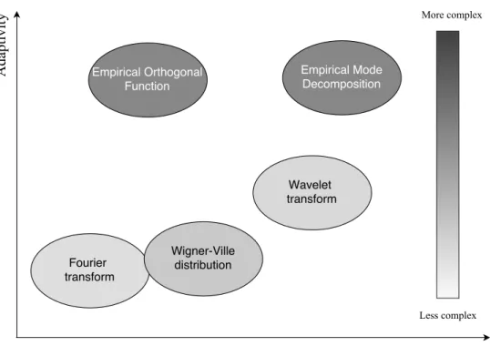
1.1 A comparative diagram to classify different data analysis methods based on
their adaptivity, robustness and complexity level. . . 4
2.1 The first iteration of sifting process after applying EMD algorithm ons(n) . 13 2.2 The upper figure shows the first sifted IMF (IMF1) in contrast to the tone s1(n) and the lower figure shows the second IMF (IMF2) in contrast to the tone s2(n) . . . 14
2.3 The first 6 IMFs and the correspondings1(n) ands2(n) tones . . . 15
2.4 The Power Spectral Density ofy(n) and the corresponding IMFs . . . 16
3.1 The distributions of IMF3 different random variable distributions. . . 27
3.2 The distributions of IMF3 different random variable distributions corrupted with wGn. . . 27
3.3 The IMF variances of different random variable distributions. . . 28
3.4 The IMF variances of different random variable distributions of corrupted with wGn. . . 29
3.5 The excess kurtosis of IMFs for different random variable distributions with
and without corruption of wGn. The grey solid lines and the black solid lines, along with their error bars, are the result of signal distributions without and with wGn respectively. The dashed lines represents the excess kurtosis
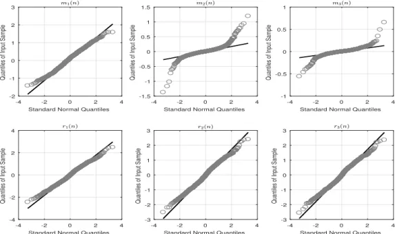
3.6 The QQ plot of the envelope mean and residual signal for three sifting
itera-tions of IMF2. . . 31
3.7 The ratio ξ for different signal distributions between the envelope mean and
residual signal for 10 sifting iterations of IMF2. . . 33
3.8 Hausdorff distance measure of the GGD for values of κ with respect to the
closed-form expression . . . 35
3.9 The effect of sampling rate and SNR variation of GGD model for an ECG
signal. . . 40
3.10 Illustrates the performance of EMD-H method in contrast with other
conven-tional de-noising techniques . . . 41
3.11 SNR comparison between EMD-H and other EMD-based de-noising methods
for various signals with 8Nq sampling rate . . . 42
4.1 The probability distribution of both upper and lower envelops of IMF1 for a
processed wGn signal . . . 49
4.2 The exponential distribution of each periodogram for IMF1 with 95%
confi-dence interval . . . 50
4.3 The schematic diagram of the proposed method . . . 52
4.4 ROC of the proposed approach for different SNR values andN = 5000 . . . 53
4.5 ROC of the proposed approach for different sample sizes and SNR =−12 dB 53
4.6 A multi-channel detection rate for different false alarm probabilities . . . 54
4.7 A comparison of the proposed method to the ED and MED under noise
un-certainty effect with N = 5000 . . . 55
4.8 The enhancement percentage of using IMF1 over the use of all IMFs in terms
of EMD processing computational complexity . . . 56
4.9 Complexity comparison of the proposed method versus ED, MED and
5.1 Normalized frequency response of IMF1 for different values of N . . . 63
5.2 The relationship betweenβ and log2(N) . . . 63
5.3 β vs. number of samples and SNR values . . . 64
5.4 No. of samples in respect to Pd . . . 67
5.5 ROC curves of ED . . . 67
5.6 ROC curves of MED and MME . . . 68
ABSTRACT
Statistical Properties and Applications of Empirical Mode Decomposition
by
Mahdi H. Al-Badrawi
University of New Hampshire, September, 2017
Signal analysis is key to extracting information buried in noise. The decomposition of signal is a data analysis tool for determining the underlying physical components of a processed data set. However, conventional signal decomposition approaches such as wavelet analysis, Wagner-Ville, and various short-time Fourier spectrograms are inadequate to process real
world signals. Moreover, most of the given techniques require a prior knowledge of the
pro-cessed signal, to select the proper decomposition basis, which makes them improper for a wide range of practical applications. Empirical Mode Decomposition (EMD) is a non-parametric and adaptive basis driver that is capable of breaking-down non-linear, non-stationary signals into an intrinsic and finite components called Intrinsic Mode Functions (IMF). In addition, EMD approximates a dyadic filter that isolates high frequency components, e.g. noise, in higher index IMFs. Despite of being widely used in different applications, EMD is an ad hoc solution. The adaptive performance of EMD comes at the expense of formulating a theoretical base. Therefore, numerical analysis is usually adopted in literature to interpret the behavior.
outcome to enhance the performance of signal de-noising and spectrum sensing systems. The novel contributions can be broadly summarized in three categories: a statistical anal-ysis of the probability distributions of the IMFs and a suggestion of Generalized Gaussian distribution (GGD) as a best fit distribution; a de-noising scheme based on a null-hypothesis of IMFs utilizing the unique filter behavior of EMD; and a novel noise estimation approach that is used to shift semi-blind spectrum sensing techniques into fully-blind ones based on the first IMF. These contributions are justified statistically and analytically and include comparison with other state of art techniques.
CHAPTER 1 Introduction
1.1 Motivation
A signal is the result of a sensor measurement or readings and it consists of useful infor-mation embedded in some level of noise. Signal examples include but are not limited to biomedical, electrical faults, health monitoring, Global Positioning System (GPS), seismic, climate, wireless communication, and mechanical vibrations. The signal received from the aforementioned examples is the link to understand the underlying features of a given process, in which signal analysis is the interpretation key of that link. On the other hand, the use of a proper signal analysis technique will result in a significant support in making a valid decision such as estimation, detection, and recognition [3]. Further, signal interpretation is necessary whether the particular measurement carry useful information or just a noise. For example, analyzing a wireless signal at a certain frequency band can help greatly to decide if that band is carrying any information or not and that is the basic concept of spectrum sensing techniques.
Practically, signals are multi-component, non-linear and non-stationary in nature, there-fore, decomposition process is the way to extract its physical meaningful components. In that sense, separating, or decomposing, such multicomponent to their basic scales is rather essen-tial to reveal the underlying physical characteristics of these measurements. Conventional decomposition techniques such as wavelet analysis, Wagner-Ville, and various short-time Fourier spectrograms are incapable of processing such signals efficiently. In addition, con-ventional techniques can either work effectively for non-linear signals or for non-stationary
signals, but none are able to accommodate for both [4]. The robustness of a decomposition method can be examined by its ability to:
• effectively decompose non-linear and non-stationary signals.
• adaptively derive the decomposition basis out of the signal itself.
• extrat the signal features in the presence of noise.
• represent the signal frequencies locally, i.e. at their time of occurence.
Generally, Fourier Spectral analysis is the most widely used approach in data interpre-tation due to its simplicity in both theory and applicability. Nevertheless, the performance of Fourier analysis approaches is captivated by several limitations such as linearity and sta-tionarity of the processed data. Moreover, and in terms of signal representation, Fourier approaches, such as Short-Time Fourier Transform STFT, (an extension of the basic Fourier
transform with short time sliding window), lack the adaptive behavior as it is based on a
priori basis and suffer from energy leakage. The Wigner-Ville function is another example of Fourier analysis in which the window is shifted copy of the processed signal itself. Be-cause this method (Wigner-Ville) is derived from Fourier analysis, thus it suffers from all constraints that Fourier analysis exhibit [5].
On the other hand, wavelet approaches represent an advanced version of Fourier Spectral methods with a predefined window in which each window (wavelet function) can be adjusted for a specific application. Although wavelets have been proved with mathematical rigor, ver-satile for different applications, and have the ability to analyze non-stationary signal, wavelet
methods are non-adaptive in which the decomposition basis are selected a priori.
Empiri-cal Orthogonal Function (EOF) is an example of a posteriori basis decomposition example
where the basis are derived from the data [6]. In this method, the basis are obtained by calculating the eigenvectors from the covariance matrix of the processed data. Despite of the orthogonality of EOF basis, its output modes do not guarantee a meaningful representation of the data in which even random processes might reveal falsely a physical pattern [7].
Thus, in order to alleviate the drawbacks of the aforementioned decomposition methods, the Empirical Mode Decomposition (EMD), which is the key component of Hilbert-Huang Transform (HHT), is adopted in this work [8]. EMD is an adaptive data driven tool with
basis that are defined a posteriori and a capability to analyze non-linear and non-stationary
signals effectively. Beside its ability to extract signal features, EMD has the advantage of decomposing signals locally and that is becomes significant when the signal varies with time. The adaptive behavior of EMD comes at the expense of formulating a mathematical frame, therefore this approach is empirical.
Fig. 1.1 illustrates a comparative diagram of different data analysis methods with respect to their adaptivity, robustness and complexity. The term, adaptivity, refers to ability of a
method to derive its basis from the processed signal itself and nota priori. On the other hand,
the term, robustness, refers to the ability of a method to extract signal features regardless of the non-linearity and non-stationarity of the processed signal. Further, the term, complexity,
refers to the arithmetic operations of an algorithm to process N samples. From Fig. 1.1, the
complexity level for Fourier transform [9], and Wavelet transform [10] are shown to be less than the EOF [11] and EMD [12] and close to Wigner-ville distribution [13].
1.1.1 Significance of EMD Statistical Properties
In recent years, EMD gained a lot of attention and has been applied in different areas because of the unique properties and the superior performance. Despite its use, successfully, in various applications, EMD still lacks a theoretical basis and is defined as an algorithm with no analytical interpretation [14]. Therefore, it is essential to understand its statistical properties and analyze its behavior to be utilized in real world applications.
Applying EMD algorithm on a time-series signal will result in a complete and finite set of components called Intrinsic Mode Functions (IMFs). The statistical characteristics of these IMFs are studied in literature and it has been conducted to have a significant influence on the way EMD is applied for various applications [3]. One of the important aspects of
Figure 1.1: A comparative diagram to classify different data analysis methods based on their adaptivity, robustness and complexity level.
understanding the behavior of EMD process led to conclude that the EMD resembles a dyadic filter (similar to wavelet) in which IMFs play the role of overlapping bandpass filters [15]. Thereafter, the filter bank properties make it more obvious that the findings of other filter bank techniques can be applied in EMD effectively. On the other hand, the investigation of the probability distribution functions of the IMFs supports such filtering features and provides insight to develop more advanced adaptive filtering methods [16].
1.1.2 Significance of Signal De-noising
The aim of de-noising is to recover useful information buried in noisy measurement pro-cesses while retain its features unaltered. However, noise is an inevitable part of any real collected data and might vary from highly correlated to uncorrelated with the corrupted signal. Different filters have been proposed such as linear filters and transform-based meth-ods. However, these techniques are vulnerable to signal changing characteristics and/or prior filter parameter assumptions [16].
Filtering through EMD comes quite natural, in which the relevant modes corresponding to the signal components (almost noise free) are separated during the sifting operation. However, selecting the relevant IMFs is a critical process especially in the presence of high noise power. Unfortunately, analytical expressions of the signal IMFs are not available. Thus, most of the important results on the EMD are all based on the empirically determined findings from numerical experiments.
1.1.3 Significance of Signal Detection
Signal detection is the process of deciding whether a certain measure (either in time or frequency domain) is occupied with information or if it comprises noise only. Cognitive radio is one of the most contemporary approaches that is relied on the concept of detection theory. Cognitive radio enables the use of radio spectrum that is underutilized due to the fix allocation of frequency bands. In the physical layer of cognitive radio, spectrum sensing plays a key role in detecting the holes (vacant channels) for a given band. Further, energy detection (ED) is used widely for spectrum sensing purposes due to its non-coherent nature and low computational complexity [17].
More recently, Empirical Mode Decomposition (EMD) has been proposed as a detection method for wireless applications. EMD works adaptively and blindly to decompose time-series signals into a set of modes (IMFs) that can be utilized for detection purposes. Similar to ED, EMD behaves non coherently towards the received signals in which it requires no prior information about the signal characteristics.
1.1.4 Significance of Noise Power Estimation
In practical scenarios, signals are corrupted with noise unavoidably. Further, the noise
power characteristics is unknown at the receiver and range from very mild (high SNR) to very severe (low SNR). If the noise power is incorrectly assumed, the spectrum energy detector for example, may result in a significant degradation in performance and might yield
in false decisions. Therefore, noise power estimation is required to mitigate the impact of the presumptions and its consequences.
Empirical Mode Decomposition algorithm can be used for noise power estimation because it has a unique ability to process noise. In wireless communications, an accurate estimation of the noise power could enhance the quality of the communication link by tuning of the transmitter and receiver parameters. Further, the knowledge of the estimated noise power can be used to calculate the SNR which is an indication of the communication channel reliability.
1.2 Dissertation Contributions
In this work, the aim is to investigate the EMD sifting process and represent the IMF’s probability distribution functions in more general representation in which the existing fitting distributions are seen as special cases. The understanding of IMF probability distributions is used for de-noising purposes in which an adaptive filter based on EMD characteristics is designed. In addition, the first IMF statistical features is utilized to propose a blind noise estimation approach that can be applied to shift semi-blind spectrum sensing methods to fully-blind ones. In this sense, the contributions of our research can be outlined as follows:
1. Modeling the Intrinsic Mode Functions of input signal distributions using Generalized Gaussian distribution (GGD) and validate that model via null hypothesis test [18]. 2. Investigating of the IMFs statistical properties when random variables of different
distributions are decomposed by EMD. The outcome of this investigation led to an important result that for an unknown distributed signal, the generated IMFs will be a set of GGD modes and residual.
3. Proposing a novel scheme for signal de-noising based on the null hypothesis of the Generalized Gaussian distribution of Intrinsic Mode Functions [18]. This includes an
evaluation of IMF models including the well-known Gaussian, Laplacian and the GGD in different scenarios and compare these models from different perspectives.
4. Proposing a multi-channel detection methods based on the behavior of Intrinsic Mode Function energies in frequency domain [1, 2]. Further, analyzing the properties of the first Intrinsic Mode Function and use its unique features for signal detection [19, 20]. 5. Proposed a novel approach for noise estimation using the characteristics of the first
Intrinsic Mode Function and apply that approach to enhance the performance of noise-dependent spectrum sensing techniques such as energy detectors [21].
1.3 Dissertation Layout
This dissertation is outlined as follows:
• Chapter 2 addresses the theoretical background of the Empirical Mode Decomposition
algorithm associated with sifting process parameters. Further, examples on the ability of EMD to sift different scales out of the composite signal is presented. On the other hand, a literature review of the EMD statistical properties is outlined followed by review of signal de-noising and spectrum sensing methods.
• Chapter 3 includes a statistical analysis of the Intrinsic Mode Functions and an
in-vestigation of its probability distribution functions. From the statistical findings, a de-noising scheme based on the null hypothesis of IMFs is proposed and examined in different scenarios for various types of signals.
• Chapter 4 covers the use of EMD properties in filtering to propose an adaptive spectrum
sensing technique. The proposed technique is blind in which it does not required a predefined parameters or a knowledge of the received signal characteristics such as the noise variance. The performance of the proposed technique is evaluated under low signal to noise ratio regimes and different sampling rates.
• Chapter 5 includes a novel noise power estimation method based on the scaling of the first IMF and use that knowledge of the noise power to shift the semi-blind spec-trum sensing techniques to blind ones. The proposed method is explained analytically and demonstrated to exhibit good performance in contrast to the other noise power estimation techniques.
• Chapter 6 covers the conclusion remarks of this dissertation including the findings and
CHAPTER 2 Background
In this chapter, the pertinent background to the performed and the proposed contributions are presented. The theoretical definition of the Empirical Mode Decomposition algorithm and its sifting process is addressed with illustration examples. A literature review of all recent and relevant findings in the EMD domain and it applications in both de-noising and detection is outlined.
2.1 Empirical Mode Decomposition: Theoretical Background
2.1.1 EMD Algorithm
Empirical Mode Decomposition is an adaptive approach that is used to analyze non-linear
and non-stationary signals. This technique decomposes time-series signals, through the
sifting process, into a complete and finite set of amplitude and frequency modulation (AM-FM) oscillatory components called Intrinsic Mode Functions (IMFs). Sifting process is the key concept of the EMD in which the iteration will continue over the processed signal until a stoppage criteria is satisfied. However, the number of iterations over each sifted IMF is a function of the signal length and its smoothness. The IMF must satisfy the following two conditions: (1) the number of extrema and the number of zero-crossings must be either equal or differ at most by one for the entire data set. (2) The mean value of the envelope defined by the local maxima and by the local minima is zero, at any point.
If y(n) was the processed signal, where n is the sample index, thus the EMD algorithm
1. Initialize the input r(n) as y(n) (the residue signal).
2. Identify extrema points of r(n): maxima and minima.
3. Interpolate maxima and minima points to form the upper and lower envelopesemax(n)
and emin(n) respectively.
4. Evaluate the mean: m(n) = (emin(n) +emax(n))/2.
5. Extract the detailed signal: h(n) =r(n)−m(n).
6. If h(n) does not satisfy the stoppage criteria, then the process is repeated andh(n) is
the input to step (2).
7. If h(n) satisfies the stoppage criteria, then h(n) is the jth IMF. The residue is y(n) =
r(n)−IMFj(n). If the number of zero crossings of the residue <2, then break the
process and keep the last collected signal as a trend. Otherwise, back to step (1) with the residue as the input.
The original input signal can be reconstructed as the sum of the IMFs and the trend such that: ˆ y(n) =T(n) + M X i=1 IMFi(n) (2.1)
where, ˆy(n) is the reconstructed signal,T(n) is the trend of y(n) (or residual) and M is the
number of sifted IMFs.
2.1.2 Sifting process parameters
EMD is an algorithmic-based technique that does not hold a rigor mathematical definition. However, the sifting process represents a unique and powerful phase of EMD that compen-sated the lacking of theoretical framework.
In the sifting process, two parameters are mainly investigated in the literature and they are given as follows:
Stoppage criteria
The stoppage criteria is suggested to halt the sifting process at a point that ensure a com-pleteness of the physical meaning for the extracted IMF. In that sense, several stoppage criteria have been proposed [8, 22, 23].
In [8], Cauchy convergence test, which is defined as a normalized squared difference (SD) between two successive sifting operations, is used such that:
SDk = PN n=0|hk−1(n)−hk(n)|2 PN n=0h 2 k−1 (2.2)
where hk is the kth extracted signal through the sifting, and k is the iteration number. If
SDk is smaller than the predetermined value (0.2∼0.3), the sifting process will be stopped.
In [22], Huang et al. suggested another stoppage criteria called S-number. S-number
is a pre-selected parameter that is is used to stop the sifting process whenever the number of zero-crossings and extrema stay same or almost differ by one after S-consecutive times.
Generally, S-Number selection is ad-hoc, however, Huang et al. established an empirical
guide, and he found that for optimal sifting, the range of S-number should be set between 4 and 8.
In [23], the authors proposed two thresholds (θ1 andθ2) approach that endeavor to retain
locally large deviations and globally small mean oscillations of the extracted IMF. For that
purpose, the authors introduced two terms namely: mode amplitude a(n), and evaluation
function η(n), such that:
a(n) = emax(n)−emin(n) 2
η(n) = |m(n)
a(n)|
η(n)<θ1 : (1−ϑ) of total IMF duration η(n)<θ2 :ϑ of total IMF duration
where the authors set ϑ≈0.05, θ1 ≈0.05 andθ2 ≈10θ1 as a default values.
Interpolation approaches
In EMD domain, the interpolation is the process of connecting the identified extrema (max-ima/minima) to form the upper and lower envelopes respectively. To this end, different interpolation approaches have been proposed aiming for more efficient decomposition
pro-cess. In [8], Huang et al. suggested the use of cubic spline interpolation to fit all maxima
(resp. minima) data points. However, Huang et al. conducted that higher order splines
required extra computational time and more parameters have to be determined and that is discrediting the adaptivity of the approach. In [24], the authors proposed the rational splines that include the cubic spline as a special case, however, this method is performing better if only the pole parameter that controls the tautness of the spline, is tuned carefully. In [25], raised cosine interpolation is proposed to provide more efficient implementation as the pro-posed approach is based on fast Fourier transform. However, this method of interpolation is dependent on the roll-off factor and the sampling period which in turns is signal-dependent leading to not a fully adaptive EMD approach.
2.1.3 Examples on EMD sifting and IMFs extraction
To further illustrate the mechanism of sifting process that led to extract IMFs, the following two examples are presented:
Example 2.1.1. In the first example, the EMD algorithm is applied on a multicomponent
signal that consist of two tones of equal amplitudes, A, and zero phase shifts in which the
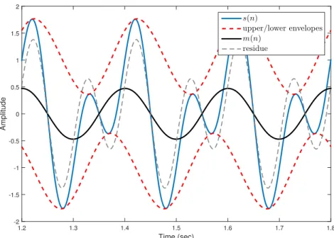
Time (sec) 1.2 1.3 1.4 1.5 1.6 1.7 1.8 Amplitude -2 -1.5 -1 -0.5 0 0.5 1 1.5 2 s(n) upper/lower envelopes m(n) residue
Figure 2.1: The first iteration of sifting process after applying EMD algorithm on s(n)
s(n) =s1(n) +s2(n)
where s1(n) and s2(n) are defined as follows:
s1(n) =Asin(2πf1t) (2.3)
s2(n) =Asin(2πf2t)
The sifting process starts by identifying the local maxima and the local minima of s(n),
then a cubic spline interpolation (3rd order) is applied to connect these extrema
(maxi-ma/minima) to form the upper and lower envelopes respectively. Subsequently, the mean,
m(n), of the upper and lower envelopes are calculated and subtracted from s(n) to obtain
the residue in which the residue is tested for stoppage criteria condition to decide whether
it is IMF or not. Fig. 2.1 illustrates the sifting process after applying EMD on s(n).
Example 2.1.2. In the second example, the signal s(n), defined in Example (2.1.1), is contaminated with a white Gaussian noise (wGn) as follows:
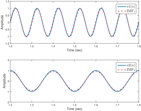
Time (sec) 1.2 1.3 1.4 1.5 1.6 1.7 1.8 Amplitude -1.5 -1 -0.5 0 0.5 1 1.5 s1(n) IMF1 Time (sec) 1.2 1.3 1.4 1.5 1.6 1.7 1.8 Amplitude -2 -1 0 1 2 s2(n) IMF2
Figure 2.2: The upper figure shows the first sifted IMF (IMF1) in contrast to the tone s1(n)
and the lower figure shows the second IMF (IMF2) in contrast to the tone s2(n)
y(n) = s(n) +w(n)
where y(n) is the noisy version of s(n) and w(n) is independent and identically distributed
(i.i.d.) white noise with zero-mean and variance σ2
w i.e. w(n) = N(0, σw2).
Similar to Example (2.1.1), the EMD algorithm is applied on y(n) and the sifting process
is shown in Fig. 2.3. From that figure, it is obvious that IMF1 carries the highest frequency
of the processed signal which is in this case the white Gaussian noise, w(n). Similarly, IMF2
and IMF3 sift the residual of the highest frequency components (mostly noise). However,
it is noticeable that IMF4 and IMF5 sifted the frequency of s1(n) and s2(n) reflecting the
behavior of dyadic filter. Herein, it becomes clear that EMD works as a natural and adaptive signal separation technique with an advantage of extracting the signal features in noisy environments.
1.2 1.3 1.4 1.5 1.6 1.7 1.8 -2 -1 0 1 2 1.2 1.3 1.4 1.5 1.6 1.7 1.8 -2 -1 0 1 2 1.2 1.3 1.4 1.5 1.6 1.7 1.8 -1 -0.5 0 0.5 1 1.2 1.3 1.4 1.5 1.6 1.7 1.8 -2 -1 0 1 2 IMF4 s1(n) 1.2 1.3 1.4 1.5 1.6 1.7 1.8 -2 -1 0 1 2 IMF5 s2(n) 1.2 1.3 1.4 1.5 1.6 1.7 1.8 -0.4 -0.2 0 0.2 IMF 1 IMF 3 IMF 2 IMF 6
Figure 2.3: The first 6 IMFs and the corresponding s1(n) and s2(n) tones
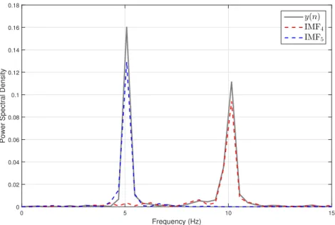
of the processed signal, y(n), and the corresponding IMFs (IMF4 and IMF5) are presented
in frequency domain. From that figure, under sufficient sampling rate (>Nyquist rate),
the EMD decomposed the processed signal from highest to lowest frequency resembling the behavior filter bank.
2.1.4 Sampling Rate Effect on EMD Performance
Originally, Empirical Mode Decomposition was designed to process continuous signals and hence any discontinuity can be misinterpreted as a signal component, thus oversampling is required for practical applications [3]. In [26], experiments have been performed to establish an EMD sampling limit. It was conducted that when the frequency of the processed signal approaches the sampling frequency, the EMD performance will degrade due to low amplitude resolution. However, it was found that a sampling frequency needs to be 5 times the Nyquist
rate (2×fmax, where fmax is the highest frequency in the processed signal) in order to sift
Frequency (Hz)
0 5 10 15
Power Spectral Density
0 0.02 0.04 0.06 0.08 0.1 0.12 0.14 0.16 0.18 y(n) IMF4 IMF5
Figure 2.4: The Power Spectral Density of y(n) and the corresponding IMFs
In [27], the authors studied the influence of the sampling on the EMD performance and illustrated possible sampling rate requirements. Moreover, the authors stated that the oversampling requirement is independent from the Nyquist criterion and is more related to reducing discontinuities in the signal. If the input to the EMD process is sampled at the Nyquist rate and an extremum (maximum/minimum pair) is lost during the sampling process thus, a local oscillation for the EMD process will not be determined in the sifting process. In [28], the proper sampling bound is selected based on a derived distribution model of white Gaussian noise whereas the deviation from this model indicates that the sampling rate is not sufficient enough to extract the information of the processed signal. In [29], the authors used a sampling rate of 50 times faster the Nyquist rate to fulfill the oversampling condition of EMD process.
2.1.5 EMD Applications
Despite of its empirical bases, EMD has gained a significant importance due to its robustness and superiority over other analogues. EMD has been applied into different data analysis fields of research, some of these fields are summarized as follows:
• Biomedical measurements: include features extractions [30, 31], de-noising [16, 18], and seizure detection [32]
• Wireless communications: include radar systems [33, 34], satellite faults diagnosis [35], overlay communications [36,37], and spectrum sensing in cognitive radio networks [1, 2, 21, 38]
• Faults analysis: include Power quality assessment [39], Damage detection [40, 41], and Structural health monitoring [42]
• Speech processing: include speech noise suppression [43], speech recognition [44], and speech watermarking [45]
• Image processing: include image analysis [46], image watermarking [47], and image
compression [48]
2.2 Literature Review
In this section, a review of the recent works that are related to our contributions and the pro-posed research is presented. This section is categorized in three different; however, coherent; areas begin with a review of the statistical analysis of the IMF properties. The de-noising problem is reviewed and the focus will be mainly on the EMD-based techniques in addition to other recent researches. In the detection category, the cognitive radio field with its key part, spectrum sensing, will be reviewed by addressing the most important related techniques.
2.2.1 Empirical Mode Decomposition: Statistical Properties Review
The EMD output mode, IMFs, and the decomposition sifting process have been investi-gated and analyzed statistically to understand its associated properties and underlying fea-tures [15, 49, 50]. Wu and Huang studied the statistical characteristics of IMFs of white Gaussian noise (wGn) and they concluded that the IMFs will approximately follow a
a similar conclusion [15]. The phrase ‘approximately Gaussian distributed’ is used by both research groups loosely and has no strict mathematical meaning.
In addition to the aforementioned attempts to determine the statistical characteristics
of IMFs, G. Schlotthauer et al. investigated the effect of the number of samples and the
number of sifting iterations on the properties of the IMFs [50]. The later research group
remarked that the probability density functions, pdf, of the IMFs are strongly dependent
on the data length and on the maximum allowed number of iterations. However, unlike the findings in [15, 49], they observed (after applying two normality test methods) that many of the collected IMFs can have a Laplacian or a multi-modal rather than a Gaussian distribution except for few cases. Tseng and Lee proposed a two step entropic method to study IMF’s properties by using a Bayesian interpretation of the resulting probabilities [28]. The two step entropic method involves in its first step clustering the resulted IMFs into two groups in which the first group contains the first set of IMFs, and the second group consists of the rest. The second step includes calculating the relative entropy between the input signal and each cluster in which minimum relative entropy indicates the presence of information.
2.2.2 Signal De-noising Review
Signal de-noising is a widely used term in signal processing which refers to removing the noise corruption to measurements such as biomedical, seismic, faults, and speech signals to name some. In this review, the focus will be on EMD-based de-noising techniques and
some of the peer techniques from different approaches. Donoho et al. proposed a method,
based on wavelet filtering, to de-noise signals by applying a soft thresholding approach on the obtained empirical wavelet coefficients and then invert the filter coefficients to recover
the smoothed signal [10]. Sameni et al. suggested the use of non-linear Bayesian filter
framework to process a single channel electrocardiogram using a modified non-linear dynamic model [51]. The modified model is utilized in several filters includes Extended Kalman Filter, and Unscented Kalman Filter with a use of automatic parameter selection method for better
model adaptation.
The advantage of understanding the statistical properties of IMFs is that signals can be de-noised more effectively, in which the relevant modes corresponding to the signal com-ponents (almost noise free) are separated during the sifting operation. However, selecting the relevant IMFs is a critical process especially in the presence of high noise power. Flan-drin et al. suggested the use of first Intrinsic Mode Function to set a noise-only model in order to use it as a threshold to decide whether the processed signal is carrying informa-tion or not [52]. In [53], the discriminainforma-tion between different modes is approached using a correlation based threshold. In [54], the energy between two consecutive reconstructions of the signal is measured and the IMF index is identified when the first significant energy change occurs. The statistical characteristic of IMFs for noise is used to calculate energy spread as a function of various percentiles; filtering is then achieved by reconstructing the IMF energies out of the spreading bounds [55]. In [56], the Hurst exponent is adopted to select the IMFs that contribute to the signal more than noise, and partial reconstruction is used to produce an enhanced speech version. In [57], EMD is exploited in cooperation with HOS for speech-stream detection in low SNR region. The statistical similarity distance between the probability distribution of IMFs is used to decide which IMFs should be used for reconstruction to reduce noise [16].
2.2.3 Signal Detection: Spectrum Sensing Review
There is a great demand for bandwidth in wireless communications due to the dramatic shift in data usage from voice only to multimedia applications. Cognitive radio systems (CR) were proposed as a solution to satisfy that demand by making under utilized spectrum available. Spectrum sensing is the key part of CR as these systems must adapt to use different spectrum and bandwidths based on a primary user’s channel usage. The efficacy of these systems relies on the ability to detect and monitor the primary users signal to avoid interference [58].
measurements namely, the probability of detection (Pd) and the probability of false alarm
(Pf a). In definition, Pd is the probability to decide the presence of signal when it is truly
exist, and can be written as follows:
Pd=P rob(H1|H1) (2.4)
On the other hand, Pf a is the probability to decide incorrectly the presence of signal
when it is indeed absent, and can be formulated as follows:
Pf a =P rob(H1|H0) (2.5)
Moreover, Receiver Operating Characteristic (ROC) curves is used to provide a
compre-hensive performance measure by providing a link between different Pd and Pf a values at
certain Signal-to-Noise Ratio (SNR).
CR consists of a broad range of spectrum sensing techniques, each of which have advan-tages and disadvanadvan-tages. These techniques range from low to high computation complexity and have varying levels of ability to determine the presence of signals in noise. An ideal
spectrum sensing technique would sense any class of signals quickly, require no a priori
information and operate at low SNR walls [17].
Energy detectors (ED) are the most popular among all spectrum sensing techniques due to its low computational complexity; in which, the energy metric of the received signal is compared to a predefined threshold to decide the occupancy of a given channel [59]. However, lacking of the accurate estimation of the noise variance may result in increased missed detection and false alarms On the other hand, noise uncertainty is additional factor that affects the efficiency of energy detectors in which noise starts to fluctuate during the sensing duration.
In [60], an adaptive multi-band energy detector accompanied with the nonparametric Kolmogorov-Smirnov (K-S) test are proposed through an iterative exploration process that reduces the number of nominee channels. Zeng and Liang proposed a spectrum sensing
methods based on the sample covariance matrix of the received signal [61]. The eigenvalues of the sample covariance matrix is calculated and thresholds are derived for the probability of detection and the probability of false alarm. An example of the eigenvalue-based detector is called Maximum-Minimum Eigenvalue detector (MME) which is independent of the noise power of the received signal and perform well in low SNR regimes. Further, another example of eigenvalue-based detectors is called Maximum-Eigenvalue Detector (MED) in which is dependent on the noise power and still performs well under low SNR scenarios [62].
In terms of spectrum sensing, EMD was used as a component of detection methods and wireless applications [63]. Roy and Doherty used EMD, in general, to enhance the detection of weak signals in the presence of noise [64]. This technique is dependent on a characteristic of EMD that would require calculations that may not make it practical for real-time sensing. In
an effort to detect signals under noise uncertainty, Bektaset al. proposed a spectrum sensing
algorithm based on relative entropy [38]. However, this method also requires a large number
of calculations to determine the classifier to separate a signal from noise. Gunturkun et al.
used the Bivariate Empirical Mode Decomposition (BEMD) to facilitate radar scene analysis for cognitive radar [33]. The proposed method takes advantage of the distinct response of intrinsic mode functions energies to the fractional Gaussian character of coherent sea clutter returns. That response is used then to set a null hypothesis that distinguish the presence or the absence of the target under test. The use EMD in wireless communication is limited to the baseband signals due to the high complexity (large number of samples) that arise with the application of bandpass or wideband signals.
2.2.4 Noise Power Estimation Review
Noise power estimation is widely used in speech, image, and wireless communications [65– 67]. The estimation can be performed either in time or frequency domain based on the associated application. In this review, we’ll focus on the noise power estimation in wireless communications and more specifically the applications to spectrum sensing in cognitive radio
networks.
In spectrum sensing, the noise power of the received signal is the key part to calculate the threshold that is used to make the detection decision. The importance of the noise power estimation becomes more obvious with the techniques such as energy detectors that are widely used in spectrum sensing due to its simplicity and efficacy. Techniques such as energy detectors and maximum eigenvalue detectors are considered to be semi-blind in which they require the knowledge of the noise power to calculate the detection threshold. However, the knowledge of the noise power is not available in practical situations and hence assuming the noise power might deteriorate the detection rate significantly [17]. Further, the noise in wireless communications is not stationary and might change over time due to the non-stationarity of channel characteristics [68]. Therefore, accurate noise power estima-tion can shift semi-blind techniques to blind region and to use their detecestima-tion capabilities more efficiently.
The estimation of the noise power in spectrum sensing has been studied in several works [69–71]. In [69], multiple signal classification algorithm is used to separate the signal and noise subspaces. In [70], the noise power is estimated by sacrificing sub-bands of the channel to be used only for the purpose of noise estimation. In [71], minimum descriptive length is used to separate the noise eigenvalues of the covariance matrix to be used in the noise power estimation. Further, the effect of the noise power estimation on the energy detectors performance is analyzed and investigate the conditions for SNR wall, which is the highest detection rate that can be achieved regardless of the length of the observation interval [72].
CHAPTER 3
Intrinsic Mode Functions: Statistical Analysis and Applications
Empirical Mode Decomposition is a non-linear, local and fully data-driven algorithm that breaks signals into a set of modes called Intrinsic Mode Functions (IMF). Yet, there is no mathematical basis for EMD and thus an interpretation of the statistical characteristics is required to understand the non-linear nature of the algorithm. Analytically, EMD acts as a dyadic filter in which the highest oscillations embedded in the signal, typically noise, are sifted in the first IMFs. This filtering property becomes certainly advantageous by knowing that EMD is non-parametric and derive its filtering basis from the signal itself (signal
de-pendent). In this chapter1, an analytic analysis of the EMD-sifting process is presented and
a probability distribution function is suggested as a best fit model for IMFs. The statisti-cal properties of the IMFs are traced analytistatisti-cally based on the EMD process of a range of random variables with different probability distributions. The statistical properties of IMFs are used to develop two applications; de-noising scheme and SNR estimation based on null-hypothesis test of IMFs probability distribution. In both applications, partial reconstruction is applied after identifying the reference IMF which carries more information than noise. To demonstrate the validity of the proposed methods, a comparison is made with other compa-rable approaches in addition to previously proposed EMD-based de-noising technique.The results showed that the proposed method offers a larger gain in both the de-noising and SNR estimation methods specifically at low signal to noise ratio scenarios.
3.1 Introduction
Data analysis is an essential part of any sensing or measurement process to extract in-formation buried in noise from the measured values. Conventional data analysis methods are typically limited by their statistical stationary assumptions made in advance about the processed signals. Methods such as the wavelet analysis, Wagner-Ville, and the various short-time Fourier spectrograms all share this disadvantage which limits the full potential for signal analysis [4].
Most of the aforementioned techniques requirea priori knowledge of the processed signal
or part of its statistical properties to be applied properly for a wide range of applications. Empirical Mode Decomposition (EMD) was proposed to alleviate the conventional techniques drawbacks. EMD is an adaptive non-parametric signal-oriented algorithm that decomposes time-series signal into a set of AM-FM modes called Intrinsic Mode Functions (IMF). These IMFs are by definition zero-mean oscillations and produced by an iterative operation called the sifting process. The key feature of IMFs is that they are derived from the signal itself and are not predefined like the basis functions for wavelet or Fourier transformations. Since the IMFs carry the physical features of the processed signal, understanding the statistical prop-erties of these modes is essential to establish an analytical interpretation of their relationship to the signal.
The probability distribution of IMFs yielded after processing a white Gaussian noise, wGn, are investigated in [49]. The authors concluded that the IMFs will approximately follow a Gaussian distribution. Similarly, the probability distribution of IMFs of processing a fractional Gaussian noise, fGn, is studied in [15] in which the authors came with a same
conclusion. The phrase “approximately Gaussian distributed” is used by both research
groups loosely and has no strict mathematical meaning.
In addition to the aforementioned attempts to determine the statistical characteristics of
of sifting iterations on the properties of the IMFs [50]. The later research group remarked that the distribution of the IMFs are strongly dependent on the data length and on the maximum allowed number of iterations. However, unlike the findings in [15, 49], they observed (after applying two normality test methods) that many of the collected IMFs can have a Laplacian distribution or a multi-modal distribution rather than a Gaussian distribution except for few cases. These previous investigations were also restricted to Gaussian distributed signals and little attention was given to signals with different distributions. In [18], the authors proposed that the generalized Gaussian distribution (GGD) would represents a better fit of IMFs probability distribution than the suggestions in [15, 49].
The advantage of understanding the statistical properties of IMFs is that signals features can be extracted, de-noised, more effectively [16, 18, 55, 56]. In [18], the null hypothesis of the GGD for each IMF is utilized to discard the modes which follow GGD and use
the other modes to reconstruct the de-noised signal. The statistical similarity distance
between the probability distributions of IMFs is used to decide which IMFs should be used for reconstruction to reduce noise [16]. The statistical characteristic of IMFs of noise is used to calculate energy spread as a function of various percentiles; de-noising is achieved by reconstructing the IMF energies out of the spreading bounds [55]. In [56], the Hurst exponent is adopted to select the IMFs that contribute to the signal more than noise, and use the reconstruction to produced an enhance speech version.
The purpose of this chapter is to provide a new statistical understanding of the sifting process which is the key operation of generating the IMFs. The contributions of this chapter include: a) a study of the statistical properties of the IMFs generated by EMD-processed ran-dom variables of different signal distributions, b) tracing the statistical analysis of the IMFs to propose a better probability distribution, and c) two EMD-based applications schemes, de-noising and SNR estimation, that leverage the statistical knowledge of the IMFs.
3.2 Statistical Analysis of The IMFs
In this section, the behavior of EMD process for different distributions of random variables inputs contaminated with/without white Gaussian noise (wGn) is studied. This analysis is
done by tracing the statistics of the IMFs, starting with IMF2 through the sifting process.
3.2.1 IMFs statistical properties for different random variable distributions
In previous work, it was concluded that the EMD of wGn will yield “approximately” Gaussian distributed IMFs for the low IMF indices [49]. However, the probability distribution of IMFs for non-Gaussian distributed input signals is still unclear. In order to fill this knowledge gap, extensive simulations were performed to investigate the probability distributions of IMFs resulting from signals with different random variable distributions. The simulation includes
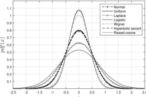
signals distributed with excess Kurtosis ranging from 3 to −1.2, which covers the following
distributions; Laplacian, hyperbolic secant, logistic, Gaussian, raised cosine, Wigner, and
uniform [73]. The chosen distributions2 also have a variety of different statistical properties.
EMD is applied on each of the random variables, a set of IMFs is generated, and the
distribution of each IMF is analyzed3. Figure 3.1 illustrates an example of a particular IMF
distribution (IMF3) of different signal distributions. From this figure, IMF3 can be seen
to follow an “approximately Gaussian distribution” with zero-mean and different standard deviations. Similar conclusion can be drawn when the same random variables are
contami-nated with wGn4 as it is shown in Fig. 3.2. At this point, the results do not contradict the
previously reported findings. This result motivates an investigation to determine if there is a distribution that fits better than “approximate Gaussian.”
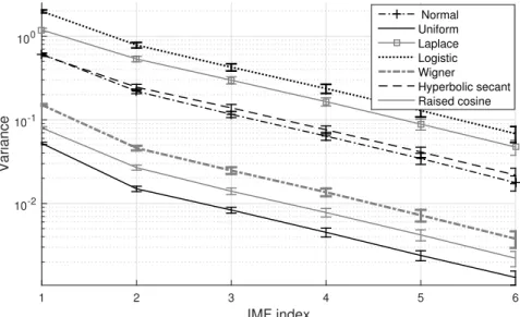
Additionally, the variance of the produced IMFs, for different signal distributions
with-2This analysis was also done for different asymmetric and non-bell shape distributions including
expo-nential, Gamma, Beta, log-normal, and Arcsine. Similar observations to the chosen distributions have been conducted.
3In this section, different random variable distributions are generated each of length of 5000 samples. The
results are the average of 100 runs based on Monte-Carlo simulations.
4As real world measurements are vulnerable to noise corruption, and because the wGn is the most common
x -1.5 -1 -0.5 0 0.5 1 1.5 p df ( x ) 0 0.5 1 1.5 2 2.5 3 3.5 4 4.5 Normal Uniform Laplace Logistic Wigner Hyperbolic secant Raised cosine
Figure 3.1: The distributions of IMF3 different random variable distributions.
x -2.5 -2 -1.5 -1 -0.5 0 0.5 1 1.5 2 2.5 p df ( x ) 0.1 0.2 0.3 0.4 0.5 0.6 0.7 0.8 0.9 1 1.1 Normal Uniform Laplace Logistic Wigner Hyperbolic secant Raised cosine
Figure 3.2: The distributions of IMF3 different random variable distributions corrupted with
wGn.
out wGn, is investigated and shown in Fig. 3.3. From that figure, it is shown that the variances decrease as the IMF indices increases because the iterative process (sifting) lowers the standard deviation of the distribution of an IMF during each iteration. Another way to understand that is the sifting process shifts the IMF distributions from platykurtic to
lep-IMF index 1 2 3 4 5 6 Variance 10-2 10-1 100 Normal Uniform Laplace Logistic Wigner Hyperbolic secant Raised cosine
Figure 3.3: The IMF variances of different random variable distributions.
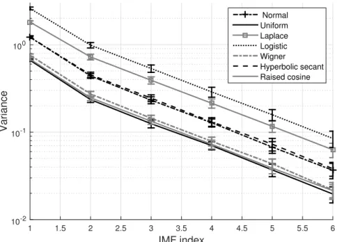
tokurtic densities and that affects the tail weight of each IMF distribution recursively which results in smaller standard deviations (variances). On the other hand, Fig. 3.4 shows the effect of corrupting the signal distributions, presented in Fig. 3.3, on the variance behavior. From that figure, it is clear that the variance values are increased in contrast to the previous figure and that is due to the contributions of the wGn variance.
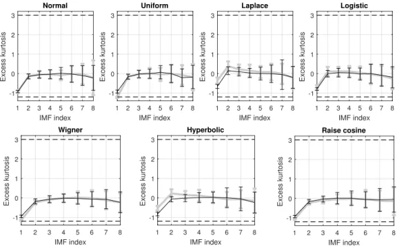
Further, the excess kurtosis of the produced IMFs is evaluated for different signal dis-tributions with and without wGn as shown in Fig. 3.5. Specifically for low IMF indices,
the excess kurtosis is about zero which indicates that the produced IMFs follow roughly a
Gaussian distribution regardless the input signals distributions. It is worthy to mention that
the excess kurtosis of IMF1 for all distributions is negative (close to -1) and that is because
the first mode is bi-modal which is known to have negative excess kurtosis [74].
Based on the aforementioned results of IMFs statistical properties, it can concluded that, for different input distributions, whether contaminated or not with wGn, the resulting IMF probability distributions will follow approximately Gaussian distribution.
On the other hand, by using excess kurtosis as a rough measure for tail weight, it is clear that the IMFs excess kurtosis demonstrates tails that can be heavier or lighter than Gaussian for different distributions [75]. Therefore, one can conclude that under varying conditions
IMF index 1 1.5 2 2.5 3 3.5 4 4.5 5 5.5 6 Variance 10-2 10-1 100 Normal Uniform Laplace Logistic Wigner Hyperbolic secant Raised cosine
Figure 3.4: The IMF variances of different random variable distributions of corrupted with wGn.
the IMFs will follow a Gaussian or other distributions. Previous work concluded that some conditions lead to Gaussian distributed IMFs and in some cases Laplacian, which is partly true. However, there is still a knowledge gap as to what the distribution of the IMFs is for all cases. Thus, in order to verify the probability distribution of these IMFs, an analysis is presented, followed by a detailed methodology to support the proposed claim.
3.2.2 IMFs probability distribution statistical analysis
In this section, the IMFs probability distribution is derived based on the analysis of the EMD sifting process. More specifically, the distribution of the envelope mean and the resid-ual signal are traced statistically. Then, an IMF candidate distribution is determined from the EMD process of the envelope mean and the residual signal. Further, a statistical dis-tance measurement is used to verify the candidate probability distribution has a better fit than previously assumed distributions. Finally, a null-hypothesis test is used to justify the suggested fitting distribution.
1 2 3 4 5 6 7 8 IMF index -1 0 1 2 3 Excess kurtosis Normal 1 2 3 4 5 6 7 8 IMF index -1 0 1 2 3 Excess kurtosis Uniform 1 2 3 4 5 6 7 8 IMF index -1 0 1 2 3 Excess kurtosis Laplace 1 2 3 4 5 6 7 8 IMF index -1 0 1 2 3 Excess kurtosis Logistic 1 2 3 4 5 6 7 8 IMF index -1 0 1 2 3 Excess kurtosis Wigner 1 2 3 4 5 6 7 8 IMF index -1 0 1 2 3 Excess kurtosis Hyperbolic 1 2 3 4 5 6 7 8 IMF index -1 0 1 2 3 Excess kurtosis Raise cosine
Figure 3.5: The excess kurtosis of IMFs for different random variable distributions with and without corruption of wGn. The grey solid lines and the black solid lines, along with their error bars, are the result of signal distributions without and with wGn respectively. The dashed lines represents the excess kurtosis boundaries (-1.2 and 3) of the uniform and Laplace distributions respectively.
For our analysis, we assume that the input, z(n) is a Gaussian random variable with
zero-mean and unity variance. The EMD algorithm is applied to z(n) and set of IMFs
is generated, IMFj. The focus of the analysis is on the second IMF as the first IMF is
deduced to follow bi-modal distribution [52]. The first iteration of the second IMF starts by
subtracting the envelope mean mi(n) from ri(n) to yield hi(n) which is the ith sifted signal
of IMF2(n). Here,mi(n) is the mean of the upper and lower envelopes of the residual signal
ri(n) which is resulting from subtracting the IMF1(n) from the input signal, z(n).
To understand how the EMD process affects the distribution of the IMFs, we consider
the distribution of the residual signalri(n) and mean of the envelopes mi(n) with a quantile
plot to assess their deviations from the theoretical normal distribution quantile. Figure 3.6 shows that the tail of the envelope mean becomes heavier (grey circles) with reference to the standard normal distribution (solid black). This is due to the sifting process changing the
-4 -2 0 2 4 Standard Normal Quantiles -2 -1 0 1 2 3
Quantiles of Input Sample
-4 -2 0 2 4
Standard Normal Quantiles -1.5 -1 -0.5 0 0.5 1 1.5
Quantiles of Input Sample
-4 -2 0 2 4
Standard Normal Quantiles -1
-0.5 0 0.5 1
Quantiles of Input Sample
-4 -2 0 2 4
Standard Normal Quantiles -4
-2 0 2 4
Quantiles of Input Sample
-4 -2 0 2 4
Standard Normal Quantiles -3 -2 -1 0 1 2 3
Quantiles of Input Sample
-4 -2 0 2 4
Standard Normal Quantiles -3 -2 -1 0 1 2 3
Quantiles of Input Sample
Figure 3.6: The QQ plot of the envelope mean and residual signal for three sifting iterations of IMF2.
data density from platykurtic to leptokurtic. On the other hand, the residual signal exhibits
tail that resembles the Gaussian distribution. Therefore, the distribution ofmi(n) and ri(n)
follow student−t and Gaussian distribution respectively; this conclusion is supported by
the best fit probability distribution simulation5. For simplicity, we’ll denote mi(n), ri(n),
and hi(n) by mi, ri, and hi respectively.
From Sec. 2.1.1, the detailed signal, hi, is the convolution of ri and mi in
frequency-domain. However, being derived from the same random variable z(n), there is a possibility
that mi and ri are statistically dependent. For dependent random variables, a copula joint
distribution is used to depict the dependency between two random variables [78]. The next step is to understand the degree of dependency in order to find the distribution of the
candidate IMF. The candidate IMF,hi, is given in terms of the joint probability distribution
5Different well-known distributions are utilized to best fit the data,m
i(n) andri(n). Bayesian information
criterion (BIC) and Akaike information criterion (AIC) are used to decide the fitting parameters that can model the underlying data. The distribution that results in smallest the BIC or AIC is assumed the best fitting distribution [76, 77].
fmi,ri by
fhi(hi) =
Z ∞
−∞
fmi,ri(mi, hi+mi)dmi (3.1)
Clearly ifmiandriare independent thenfmi,ri(mi, ri) =fmi(mi)fri(ri) and (3.1) becomes
a convolution integral.
If mi and ri are assumed to be dependent variables, thus the multivariate cumulative
distribution function F(mi, ri) = C Fmi(mi), Fri(ri)
, where C is the copula, Fmi(mi) and
Fri(ri) are the cumulative marginal distributions of mi and ri respectively. In this respect,
two statistical nonparametric measures of dependence; Kendall’s tau (τ) and Spearman’s
rho (ρ) are defined such that τ(mi, ri) = 4E[C(U, V)]−1 andρ(mi, ri) = 12E[C(U, V)]−3,
where U,V∼ Uniform(0,1), U = F(mi) and V = G(ri), F and G are the marginal
distri-butions of mi and di respectively [79]. In this work, the ratio, denoted by ξ, of ρ(mi, ri)
to τ(mi, ri) is used as an indicator to show the degree of dependency of the joint
distri-bution between mi and ri. In [80], it was conducted that the ratio ξ approaches 3/2, for
infinite number of samples, as the joint distribution approaches that of two independent random variables.
In Fig. 3.7, an analysis of the ratioξ for different signal6 distributions of IMF
2(n) is
illus-trated. From this figure, the value ofξ is approaching 3/2 over all iterations. Therefore, the
dependency can be assumed weak and approaching independence for which the convolution
integral is a good approximation for hi [80].
Given that mi and ri can be assumed to be independent and they are convoluted, then
the IMF candidate distribution can be traced statistically. Nason et al. derived a general
closed-form expression for the convolution of student−t and a Gaussian distribution [81],
6Random variables of different distributions with 5000 samples each are averaged from 1000 trails using
1 2 3 4 5 6 7 8 9 10 Iteration # 1.4 1.42 1.44 1.46 1.48 1.5 1.52 Normal Uniform Laplace Logistic Wigner Hyperbolic secant Raised cosine
Figure 3.7: The ratio ξ for different signal distributions between the envelope mean and
residual signal for 10 sifting iterations of IMF2.
which is given as follows:
ψ(x) = b πexp(a/2) " (1−a)cos(µa+ pb 2 sin(µa) IC1(p, d) + ((1−a)sin(µa)− pb b cos(µa) IS1(p, d) +be−d 2 /2 # (3.2) where a=σ−2, b=√2/σ, d=a/b, p=µb, IC1(p, d) = Z ∞ d cos(px)e−x2dx= √ π 2 e −p2/4 [1−Re{erf(c)−erf(c−d)}], and IS1(p, d) = Z ∞ d sin(px)e−x2dx= √ π 2 e −p2/4 Im{erf(c−d)},
where c = ip/2, i = √−1, Re and Im extract the real and imaginary parts, erf(.) is the
error function.
However, Nason et al. did not specify the resulting distribution of his derived
closed-form expression given in [81]. The probability distribution function of a Gaussian distribution is given as follows,
g(x) = √1 2πσe
−(x−µ)2/2σ2 (3.3)
where µand σ are the mean and the standard deviation respectively [82].
Intuitively, replacing the shape parameter of the Gaussian distribution (κ = 2) by a
variable creates a statistical family called Generalized Gaussian Distribution (GGD) [82].
This family includes the Laplacian and Gaussian distributions, κ =1 and 2 respectively, as
a special cases. The probability distribution function of a symmetric GGD is,
f(x) = κ 2ρΓ(1/κ)e
−(|x−µ|/ρ)κ (3.4)
where κ is a parameter that controls the distribution tail, ρ is defined as
q
Γ(κ1)/Γ(3κ)σ,
and Γ(.) is gamma function. Further, the GGD is suggested to model non-Gaussian
pro-cesses, where the tail weights could be heavier or lighter than Gaussian based on the shaped parameter [83].
In order to show that GGD is a better fitting distribution than Gaussian with respect to the closed-form (3.2) solution, the Hausdorff distance measure is calculated for the two distributions. The Hausdorff distance measure is calculated by,
HD(A, B) = max D(A, B),D(B, A) (3.5)
where D(A, B) = max
a∈A minb∈B||a −b|| and D(B, A) = maxb∈B mina∈A||b− a|| [84]. To calculate
Hausdorff distance for this comparison, the distribution of closed-form expression (3.2) and
GGD (3.4) will be substituted into equation (3.5) instead ofAandB respectively, as follows:
HDψ(x), f(x)=max
Dψ(x), f(x),Df(x), ψ(x)
(3.6)
Shape parameter (κ) 1.4 1.5 1.6 1.7 1.8 1.9 2 Hau sd or ff d is tan ce 2 3 4 5 6 7 8 9 Gaussianity threshold Hausdorff measure
Figure 3.8: Hausdorff distance measure of the GGD for values of κ with respect to the
closed-form expression
to determine whether there is a distribution that reveals better fitting to the closed-form
expression (3.2) than the Gaussian. From Fig. 3.8, it is clear that at (κ= 1.64), the shortest
distance or the highest similarity of GGD with respect to closed-form expression is obtained.
Further, it is obvious that the κ values in the region under the “Gaussianity threshold”
represent the closed-form expression better than the best fit Gaussian model.
The generalization of GGD includes platykurtic densities that span from the normal
density (κ= 2) to the uniform density (κ =∞) and a leptokurtic densities that span from
the Laplace (κ= 1) to the normal density (κ= 2) [83]. Thus, the GGD successfully explains
the previous findings [15, 49, 50], where Laplace and Gaussian distributions are just special cases in GGD family.
3.2.3 The null hypothesis test of GGD
The analytical analysis in Sec. 3.2.2, suggests that the EMD-processing of Gaussian dis-tributed random variable leads to a GGD. Therefore, to verify the validity of the suggested