A Data-driven Approach with Uncertainty
Quantification for Predicting Future Capacities
and Remaining Useful Life of Lithium-ion Battery
Kailong Liu,
Member
,
IEEE
, Yunlong Shang,
Member
,
IEEE
, Quan Ouyang, and Widanalage Dhammika
Widanage,
Member
,
IEEE
,
Abstract—Predicting future capacities and remaining useful life (RUL) with uncertainty quantification is a key but challenging issue in the applications of battery health diagnosis and management. This paper applies advanced machine-learning techniques to achieve effective future capacities and RUL prediction for lithium-ion batteries with reliable uncertainty management. To be specific, after us-ing the empirical mode decomposition (EMD) method, the original battery capacity data is decomposed into some intrinsic mode functions (IMFs) and a residual. Then the long short term memory (LSTM) sub-model is applied to estimate the residual while the gaussian process regres-sion (GPR) sub-model is utilized to fit the IMFs with the uncertainty level. Consequently, both the long-term depen-dence of capacity and uncertainty quantification caused by the capacity regenerations can be captured directly and simultaneously. Experimental aging data from different batteries are deployed to evaluate the performance of pro-posed LSTM+GPR model in comparison with the solo GPR, solo LSTM, GPR+EMD and LSTM+EMD models. Illustrative results demonstrate the combined LSTM+GPR model out-performs other counterparts and is capable of achieving ac-curate results for both 1-step and multi-step ahead capacity predictions. Even predicting the RUL at the early battery cy-cle stage, the proposed data-driven approach still presents good adaptability and reliable uncertainty quantification for battery health diagnosis.
Index Terms—Electric vehicles, lithium-ion batteries, data-driven approach, remaining useful life, uncertainty management.
I. INTRODUCTION
Manuscript received Oct 2, 2018; revised Oct 11, 2019; accepted Jan 31, 2020. This work was supported by the EU-funded project ”Silicon based materials and new processing technologies for improved lithium-ion batteries (Sintbat)” No. 685716, the National Natural Science Foundation of China No. 61903223, as well as the Shandong Provincial Key Research and Development Program (Major Scientific and Tech-nological Innovation Project ) No. 2019JZZY010416. Paper no. 18-TIE-3276.(Corresponding authors: Kailong Liu, Yunlong Shang)
K. Liu and W. D. Widanage are with the Warwick Manufactur-ing Group, University of Warwick, Coventry, CV4 7AL, United KManufactur-ing- King-dom (e-mails: [email protected], [email protected]; [email protected]).
Y. Shang is with the School of Control Science and Engi-neering, Shandong University, Shandong 250061, China (e-mail: [email protected]).
Q. Ouyang is with the College of Automation Engineering, Nanjing University of Aeronautics and Astronautics, Nanjing 211100, China (e-mails:[email protected]).
L
Ithium-ion (Li-ion) batteries have become the main power sources to actuate electric vehicles (EVs) [1]. One key but challenging issue in the applications of Li-ion batteries is to monitor capacity degradation and predict the remaining useful life (RUL). In real applications, the capacity of Li-ion battery would gradually degrade over repeated charging and discharging cycles until the end-of-life (EOL). After EOL, both battery’s power and capacity would drop much faster, further to cause operational impairment and even catastrophic occurrence. Therefore, an aged battery should be replaced before its capacity reaches the EOL. It is vital to develop the proper battery health diagnosis system (BHDS) to ensure that the batteries are operated within the reliable conditions.As one key function of the BHDS, a well-designed future capacities and RUL prediction strategy should not only predict the battery capacity variation but also report the uncertainty level of predicted values, further enabling EV users to make reasonable decisions to avoid unexpected failures and losses [2]. However, it is difficult to obtain a satisfactory result for capacities and RUL prediction due to the complicated and highly non-linear trajectory of battery capacity degradation.
To date, various strategies have been proposed to achieve reasonable battery future capacities and RUL prediction in the literatures. These strategies can be classified into two main categories including the specific model-based approach and data-driven approach.
For the specific model-based approach, a suitable model with the priori knowledge of battery, such as the electro-chemical model [3], Brownian motion model [4], along with observers such as Kalman filter [5] and particle filter [6], [7], are used to capture the battery fading dynamics. Although these approaches have been widely applied in the area of battery RUL prediction, several drawbacks still exist as: 1) it is difficult to accurately adjust model parameters in whole cyclic process. 2) observer technique, such as particle filter, is easy to suffer from particle impoverishment problem, which will lead to inaccurate RUL prediction. Based upon a large number of battery aging tests, cycle-life models also become another hot research field to predict battery RUL [8]. Through portraying the capacity degradation as the functions of current rate, state-of-charge (SOC), and temperature etc., these methods seem easy to be implemented. However, to some extent, they belong to open-loop type model without strong generalization ability. Data-driven approach, which does not assume any battery
degradation mechanism a priori, has also been widely adopted. On the basis of battery historical cycling data, various in-telligent techniques such as vector machine [9], [10], neural network [11], [12], autoregressive modeling [13], Bayesian prediction [14]–[16], and Box-Cox transformation [17] have successfully been applied for battery future capacities and RUL prediction. For these applications, most approaches ad-dressed the original capacity signals without considering the self-regeneration phenomena directly. These capacity regener-ation phenomena can be seen as a sudden flucturegener-ation in the available capacity occurs during battery degradation, which are mainly caused by the electrochemical cell relaxation (changes of lithium distribution homogeneity) after a pause or idle period [18], [19]. In any case, accounting for regeneration phenomena is necessary for the uncertainty quantification of further capacities prediction [18]. Besides, as pointed out by related publications [20], [21], battery capacity experiences a long-term degradation over hundreds of cycles. The degrada-tion informadegrada-tion among these cycles is highly related. How to capture these correlations so as to achieve an accurate long-term capacity prediction with reliable uncertainty management is still an open but challenging technical issue.
In this regards, several machine-learning approaches appear to be promising for handling the long-term dependence and discontinuous regenerations. Recurrent neural network (RNN) is one powerful method to extract and update the correlations of sequential data, owing to its structure by augmenting recurrent links to hidden neurons [22]. Recently, based upon the time-varying current/voltage instantiations, You et al. [23] applied RNN to achieve flexible and robust prediction of battery capacity. Zhang et al. [24] proposed a LSTM RNN-based framework to capture the long-term degradation trend. However, the confidence ranges of predicted values cannot be generated through using solo LSTM. Compared with LSTM, GPR is derived from the Bayesian framework, so the predicted battery capacities can be directly expressed with the uncertainty range [21], [25]. Therefore, for the local capacity regenerations, GPR leads to a suitable candidate for uncertainty quantification. Therefore, it is meaningful to combine LSTM and GPR for battery capacity prediction with the purpose of achieving the benefits of both these techniques. Driven by the above purpose, this paper applies the machine-learning techniques to derive a new data-driven ap-proach, enabling accurate future capacities prediction and reliable uncertainty management for Li-ion batteries. Specifi-cally, several key contributions are made as follows: 1) after using the EMD technique to decompose the original capacity degradation data for different batteries, LSTM sub-model is applied to fit the residual, bringing the benefits that the long-term dependence of battery capacity degradation can be kept and updated without gradient vanishing. 2) GPR sub-model is used to capture the local fluctuations, where the uncertainty quantification caused by the capacity regeneration phenomena can be considered simultaneously. 3) prediction performance of several data-driven models are investigated and compared in terms of kernel function and training input number. The combined LSTM+GPR model presents to outperform other counterparts. 4) for various applications including 1-step,
multi-step and early RUL predictions, the proposed data-driven approach is capable of offering highly accurate results with reliable uncertainty management. 5) Obviously, without any battery mechanism knowledge, the proposed approach can be easily extended to other battery types for health diagnosis.
The remainder of this paper is organized as follows: Section II presents the battery capacity degradation dataset. Section III describes the adopted machine-learning techniques, followed by several performance comparison tests in Sec-tion IV. SecSec-tion V analyses the experimental predicSec-tion results of the proposed approach. Finally, Section VI concludes this study.
II. BATTERY CAPACITY DATASET
Suitable battery capacity datasets play important roles in the evaluation of prognostics methods [4]. In order to evaluate the abilities of our proposed method to capture long-term depen-dence and particularly uncertainties casued by the capacity regenerations in various operating conditions, several cyclic test datasets of NASA batteries [26] and CALCE batteries [20] with strong local fluctuations and dissimilar capacity curves are selected in this study. Reasonability of using all these battery data to design ageing prognostic methods has been proven in many related work [10], [12], [19].
TABLE I
DETAILED OPERATIONAL PROFILES OF ALL BATTERIES. Battery No. Vup Vlow Ich Idis Tamb Cnew
[V] [V] [A] [A] [oC] [Ah] B05 4.2 2.7 1.5 2 24 1.86 B06 4.2 2.5 1.5 2 24 2.04 B18 4.2 2.5 1.5 2 24 1.85 B54 4.2 2.2 1.5 2 4 1.17 B55 4.2 2.5 1.5 2 4 1.32 C16 4.2 2.7 0.6 1.1 25 1.12 C38 4.2 2.7 0.7 0.7 25 1.15
Table I illustrates the operational profiles of these bat-teries. For NASA batteries, a test bench that consists of the programmable electronic load, power supply, temperature chamber and computer is used to conduct the battery cyclic aging tests. Three cells (B05, B06 and B18) that operate under 24oC ambient temperature Tamb are labelled as ’Case
1’ batteries. Another two cells (B54 and B55) with 4oC Tamb
are labelled as ’Case 2’ batteries. For CALCE batteries, all tests were conducted by using the Arbin BT2000 system, PC and temperature chamber. More details regarding the NASA test bench and CALCE test bench can be found in [27] and [20], respectively. All batteries were recurrently tested through the operational profiles including constant-current constant-voltage (CCCV) charging and constant-current (CC) discharging. The detailed values in terms of upper cut-off voltage Vup, lower cut-off voltage Vlow, constant charging
currentIch, constant discharging currentIdis,Tamb and fresh
capacityCnew for each cell are described in Table I.
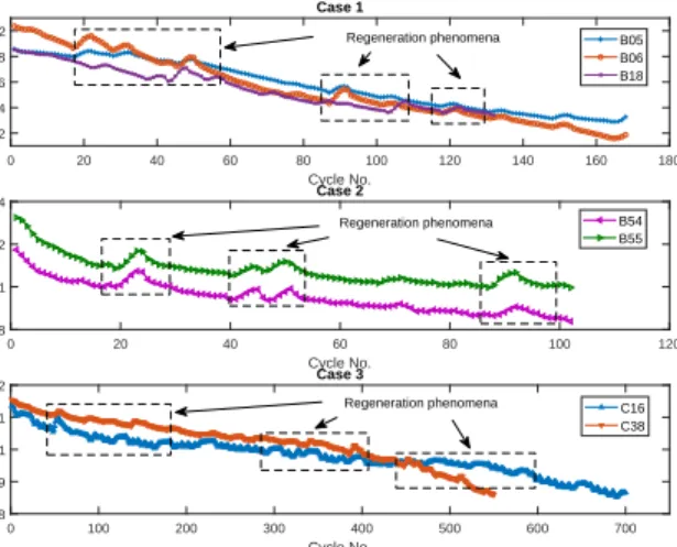
Through using the Savitzky-Golay filter to reduce measure-ment noises of corresponding currents and voltages [28], final capacity degradation curves versus cycle number for different batteries are shown in Fig 1. It is evident that the battery
0 20 40 60 80 100 120 140 160 180 Cycle No. 1.2 1.4 1.6 1.8 2 Capacity[Ah] Case 1 B05 B06 B18 0 20 40 60 80 100 120 Cycle No. 0.8 1 1.2 1.4 Capacity[Ah] Case 2 B54 B55 0 100 200 300 400 500 600 700 Cycle No. 0.8 0.9 1 1.1 1.2 Capacity[Ah] Case 3 C16 C38 Regeneration phenomena Regeneration phenomena Regeneration phenomena
Fig. 1. Original capacity degradations versus cycle number for different batteries.
capacity degradation displays a non-monotonic decline over the cycle number. Capacity regeneration phenomena and local fluctuations occur in the cyclic process. According to [21], these short-term capacity regenerations commonly occur in real-world applications. Therefore, these datasets are suitable for developing the effective capacity and RUL prognostic approaches to consider the uncertainty quantification caused by local capacity regenerations during the cycling process.
III. TECHNIQUES
To achieve reliable future capacities and RUL prediction, three points need to be concerned. First, the original capacity dataset presents a highly-nonlinear trend with regeneration phenomena, which is not suitable for accurate health prog-nosis. Second, learning the correlations of the capacity time-series is essential to update long-term dependencies. Third, uncertainty level is a key part and should not be ignored.
To solve these challenges, the proposed data-driven ap-proach mainly uses three techniques: EMD method to decom-pose the original capacity dataset, LSTM sub-model to capture the long-term dependence, and GPR sub-model to generate the uncertainty of each prediction result.
A. Empirical mode decomposition
EMD is an effective signal process technique and has been applied in many real-world fields (e.g., ocean waves, rotating machinery), owing to its strong abilities of extracting both low and high frequency components from highly dynamic signals [29]. By using EMD through an iterative sifting process, non-stationary dataset can be decomposed into a residual sequence and a series of IMFs which stand for the orthogonal-basis components. Specially, an IMF needs to satisfy several criteria as: 1) for the whole dataset, the number of zero-crossings requires to be equal to or at most one different with the number of extrema; 2) at any point, the envelopes defined by the local extrema must generate a zero mean. More details of EMD can be found in [29].
Given that the regeneration phenomena and local fluctua-tions can be considered as the high-frequency signals while the global trend of capacity degradation is the low-frequency signal, the original capacity degradation dataset will be de-composed into several IMFs and a residue by using the EMD method. Detailed sifting process to decompose the capacity dataset is described as follows,
Fori= 1toimax do
1) Setting the datasetCbat. For the first sifting process, the
original battery capacity data is selected asCbat.
2) Searching all local maxima and minima in the Cbat
through the comparisons among the adjacent values within all fluctuations. Here a local minimum or maximum value stands for a smallest or largest data point during a local scale of fluctuation [29]. Then connecting these local extrema by using the spline line to construct a upper envelop eup and a
low envelopelow, respectively.
3) Calculating the local mean by:
me= (eup+elow)/2 (1)
4) Calculating the difference betweenCbat andmeas:
dc =Cbat−me (2)
5) Setting the IMF pool by checking whetherdcsatisfies the
IMF’s criteria. Ifdc is justified to be an IMF signal, remove
this dc from Cbat to obtain the corresponding residue rc by
(3). The obtainedrc will also be denoted as the new Cbat in
next sifting process.
rc=Cbat−dc (3)
6) Repeating 2) to 5) until the obtained residuercbecomes a
monotonic function. If the predefined numberimaxis reached,
the sifting loop will be terminated.
Following this shifting process, the information of capacity regenerations have been contained in the IMFs [19]. After obtaining nIMFs along with a monotonous residuerm,Cbat
can be consisted by:
Cbat=
Xn
j=1IM Fj+rm (4)
B. Long short-term memory model
To alleviate the gradient exploding and vanishing problems, a LSTM block is generally applied to embed three gates into the hidden neurons of the RNN [22]. In this sense, one benefit of LSTM framework is that the key information can be stored or updated by manipulating the introduced gates. Besides, the LSTM model is capable of keeping information over a long period without gradients vanishing.
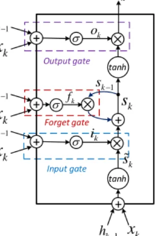
A typical LSTM-based RNN model can be divided into three gate parts, as illustrated in Fig 2. The states of all these gates are determined by thexk(the input at the current instant k) andhk−1(the output at the previous instantk−1) through
a sigmoidal unit. The input gate decides whether a new state information s˜k can be received by RNN model. The forget
gate is responsible for forgetting the previous statesk−1in the
+ k
x
1 k h tanh
k s + ks
k1 s tanh
k h + + ok + Output gate kx
1 k h Forget gate kx
1 k h kx
1 k h Input gate k f k iFig. 2. Structure of LSTM-based RNN model.
calculated by the RNN model can be output as hk. Detailed
procedure in each gate part can be summarized as:
Step 1: For the input gate part, updating the states for ˜sk
and input gateik as:
˜
sk= tanh (Wsxk+Ushk−1+bs)
ik =σ(Wixk+Uihk−1+bi)
(5) Step 2:For the forget gate part, updating the forget gatefk
and calculating the statesk as:
fk =σ(Wfxk+Ufhk−1+bf) sk =ik⊗s˜k+fk⊗sk−1
(6) Step 3: For the output gate part, updating the output gate
ok and calculating the output statehk as:
ok=σ(Woxk+Uohk−1+bo)
hk=ok⊗tanh(sk)
(7) where ⊗ means the elementwise multiplication.σ andtanh
are the activation functions of sigmoid and hyperbolic tangent, respectively. W∗ and U∗ stand for the corresponding weight
matrices. b∗ means the corresponding bias vectors.
In our study, long-term dependence represents the corre-lations among the current capacity and historical capacities during the long-term periods of battery degradation. It should be known that the capacity degradation dataset generally covers hundreds of battery operation cycles, and the degra-dation information among these cycles is highly related. In order to accurately capture the decline trend of capacity, the correlations among capacity degradation time-series data require to be taken into account via effective learning of long-term dependencies. To this end, the residual sequence will be captured by the LSTM, bringing the benefits that capacity decline information can be kept and updated without causing gradient vanishing issue.
C. Gaussian process regression model
A GPR model can be seen as an effective approach to undertake regression with the Gaussian processes [30]. A probability distribution of GPR can be denoted as:
f(k)∼GP R(m(k), κ(k, k0)) (8)
where m(k) and κ(k, k0) stand for the mean function and covariance function respectively.
In practice, there are many kernel functions that can be selected for κ(k, k0). For battery RUL prediction, a suitable kernel function has a strong impact on the prediction perfor-mance and is therefore required to be carefully selected.
One popular kernel function for GPR is the squared expo-nential (SE) function as:
κSE(k, k0) =σ2SEexp −(k−k0)2 2l2 SE ! (9) whereσSEandlSEare scaling factors to control the amplitude
and spread of the covariance, respectively.
Another common kernel function is the Matern function, as shown by: κM A(k, k0) =σ2 21−γ Γ (γ) p 2γ(k−k 0) ρ γ <γ p 2γ(k−k 0) ρ (10) where γ is a hyperparameter to reflect the smoothness. <γ
represents the Bessel function. A widely used Matern covari-ance is the Matern52 (M52) which is obtained by fixing the value ofγ as 5/2.
Adding together some SE kernels with various length scales, a new popular kernel function named Rational Quadratic (RQ) is obtained as: κRQ(k, k0) =σRQ2 1 + (k−k0)2 2αl2 RQ !−α (11) whereαreflects the relative weights of both large and small scale variations.σRQ andlRQ are hyperparameters that affect
the axis scaling.
For a regression process, the output is modeled by a function plus an additive noiseε∼N 0, σ2
n
. Then the prior distribution of observations can be denoted as:
y∼N 0, κ(k, k0) +σn2In
(12) Supposing the new dataset k0 follows a similar Gaussian distribution with the labelled training setk, the total joint prior distribution of known outputsy and predicted outputsy0 will
be expressed as: y y0 ∼N 0, κ(k, k) +σ2 nIn κ(k, k0) κ(k, k0)T κ(k0, k0) (13) Then the outputs can be predicted by calculating the con-ditional distributionp(y0|k, y, k0)as:
p(y0|k, y, k0) =N(y0|m0,cov (y0)) (14) where ( m0 =κ(k, k0)T κ(k, k) +σ2 nIn −1 y cov (y0) =κ(k0, k0)−κ(k, k0)T κ(k, k) +σ2 nIn −1 κ(k, k0) (15) It should be known that p(y0|k, y, k0) also follows the Gaussian distribution. m0 can be seen as the predicted value ofy0.cov(y0)is a covariance matrix to reflect the uncertainty.
In our work, the local regeneration and fluctuation phe-nomena in the capacity degradation dataset are high-frequency signals with large uncertainties. The GPR model is applied to fit the IMFs, while the uncertainty of predicted high-frequency values can be also considered by the covariance matrix. Here the uncertainty quantification is mainly related to the ’scope compliance’ uncertainty, which quantifies ’how confident’ the prediction from model is [31]. Such uncertainty would become larger when model performs prediction at previously unknown conditions [30].
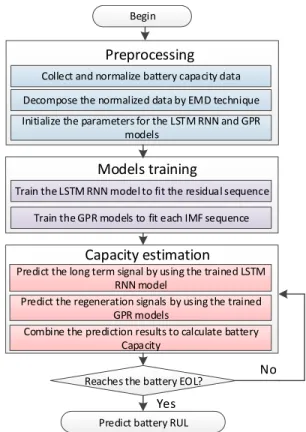
D. Implementation of data-driven approach for battery capacity and RUL prediction
The framework and flowchart for predicting future capacity and RUL based on the combined LSTM+GPR model are summarized in Fig. 3 and Fig. 4, respectively.
…
Hybrid data-driven model
Cbat(t) … Cbat(t-i) Cbat(t+k) Cbat(t-1) RULbat EM D GPR LSTM + Iteration IMFs Residual …
Hybrid data-driven model
Cbat(t) … Cbat(t-i) Cbat(t+k) Cbat(t-1) RULbat EM D GPR LSTM + Iteration IMFs Residual
Fig. 3. Framework for predicting future capacity and RUL based on the proposed data-driven model.
The model framework can be divided into two parts. For the future capacity prediction, with the current and historical capacity vector[Cbat(t−i), ..., Cbat(t)]as model inputs, output Cbat(t+k) can be predicted after employing the GPR and
LSTM to study potential mappings of the corresponding IMFs and residual. Here k andi stand for the future and previous steps, respectively. For the RUL prediction, a recursive predic-tion process that utilizes the previously predicted capacity as the next input of model to further predict new capacity value, is conducted iteratively until the battery’s EOL is reached. Then the corresponding RU Lbat can be calculated. It should
be known that the prediction is conducted just based on the historical capacity information. Detailed steps of whole prediction procedure are illustrated as follows,
Step 1: Preprocessing data and models: for data pre-processing before any training process, a simple but efficient normalization method [32] is utilized to convert the raw capacity data Cb to a normalized scale C
0
b by computing
equation:v0 =v/Cnew. HereCnewis the fresh capacity value
of a battery.v0 andvrepresent the data points inCb0 andCb,
respectively. Then the data would be decomposed into several IMFs and a residual by using EMD technique. For model part, select the suitable kernel functions for GPR. Set the structure and initialize the parameters for both LSTM and GPR models. Step 2: Training models: for a decomposed residual se-quence, train the LSTM RNN model to fit the residual sequence. For the obtained IMFs, Train the GPR models to fit each IMF sequence.
Step 3: Estimating battery future capacities: for the long term signal part, use the well-trained LSTM model to predict
Begin
Collect and normalize battery capacity data Decompose the normalized data by EMD technique
Reaches the battery EOL? Preprocessing
Models training
Train the LSTM RNN model to fit the residual sequence Train the GPR models to fit each IMF sequence
Predict the long term signal by using the trained LSTM RNN model
Predict the regeneration signals by using the trained GPR models
Capacity estimation
Combine the prediction results to calculate battery Capacity
Yes
Predict battery RUL
Initialize the parameters for the LSTM RNN and GPR models
No
Fig. 4. Flowchart for predicting battery capacity and RUL by combining the LSTM RNN model and GPR model.
the future residual value. For the regeneration signal part, apply the well-trained GPR models to predict the mean and covariance values of each IMF. After combining these results, the predicted battery capacity along with the corresponding uncertainty quantification can be obtained.
Step 4: Predicting battery RUL: calculate the battery ca-pacity in the EOL condition asCEOL. Repeat the prediction
step until the predicted battery capacity degrades belowCEOL.
Then output the predicted battery RUL.
Following this procedure, the battery capacity in each future cycle can be estimated. The RUL value is also predicted to provide valuable information for the maintenance decision for the aged battery, while the uncertainty of predicted results can be considered accordingly.
IV. DECOMPOSITION RESULTS AND PERFORMANCE
COMPARISON
In this section, the raw B18 capacity is decomposed by EMD as illustration, followed by two tests to quantify the effects of various kernel functions and number of input terms. Then, a comparison of different data-driven models are con-ducted to examine their prediction performance. Here, all the tests are implemented in Matlab 2018 with a 2.40 GHz Intel Pentium 4 CPU. For all these tests, GPRs are all trained based on the optimization of hyperparameters through using the gradient methods to maximize the log marginal likeli-hood. While the LSTM is also trained based on the gradient descent-based optimization algorithm. The effectiveness of these training ways have been proven in [24], [30]. In all relevant graphs, blue lines mean the real measured data, and
grey-background areas indicate the 95% confidence range to evaluate the reliability of the prediction results.
A. EMD decomposition result
0 20 40 60 80 100 120 140 Cycle No. -0.05 0 0.05 IMF1 0 20 40 60 80 100 120 140 Cycle No. -0.05 0 0.05 IMF2 0 20 40 60 80 100 120 140 Cycle No. 1.4 1.6 1.8 Residual value
Fig. 5. IMF and residual sequences for B18 after EMD decomposition.
After decomposing the raw sequence data by EMD, two ex-tracted IMF sequences and a residual sequence can be obtained with a low computational effort of just 0.13s. Fig. 5 illustrates the corresponding decomposition results. Specifically, the local fluctuations have been removed by EMD and the obtained residual presents an overall monotonous trend to describe the long-term dynamics. Meanwhile, all local fluctuations corresponding to the regenerations of capacity are captured by two IMF sequences. In general, IMF1 owns more fluctuations, while the trend of IMF2 is relatively gentle. As a result, more degradation information can be considered for improving the performance of battery health prognostics.
B. Kernel function and training input selection
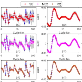
0 50 100 Cycle No. -0.05 0 0.05 IMF1 SE M52 RQ 0 50 100 Cycle No. -0.05 0 0.05 IMF2 0 50 100 Cycle No. -0.05 0 0.05 IMF1 0 50 100 Cycle No. -0.05 0 0.05 IMF2 0 50 100 Cycle No. -0.05 0 0.05 IMF1 0 50 100 Cycle No. -0.05 0 0.05 IMF2 (a1) (a2) (b1) (b2) (c1) (c2)
Fig. 6. Results for IMFs by using various kernel functions. (a) SE, (b) M52, (c) RQ
For the GPR model, selecting an appropriate kernel function is a key step. Three popular kernel functions including SE, M52 and RQ are compared to evaluate their performance for
fitting IMFs. In this subsection, all data of B18 are used to train the model, and the well-trained model is also validated under the same dataset of B18. The results by using different kernel functions are shown in Fig. 6. It is evident that for the IMF2, both M52 and RQ functions capture the whole fluctuation trend nicely. SE function is capable of capturing IMF2 before 70 cycles, after which the performance reduces with the increased confidence range. For the IMF1, SE and M52 functions achieve poor results with large uncertainties and low accuracies especially after 80 cycles. From Fig. 6(c1), the result by using RQ function is quite good, as indicated by the better match between the mean values and the true data. This is mainly due to the different length-scales capturing ability of RQ. Therefore, RQ function is selected as the kernel function for GPR model in the following study.
0 10 20 30 40 50 60 70 80 90 100 Cycle No. -0.05 0 0.05 IMF1
InNo.=6 InNo.=8 InNo.=10 InNo.=12
0 10 20 30 40 50 60 70 80 90 100 Cycle No. -0.04 -0.02 0 0.02 0.04 IMF1 0 10 20 30 40 50 60 70 80 90 100 Cycle No. -0.05 0 0.05 IMF1 0 10 20 30 40 50 60 70 80 90 100 Cycle No. -0.05 0 0.05 IMF1 (a) (b) (c) (d)
Fig. 7. Results for IMF1 by using different input number. (a) InNo.=6, (b) InNo.=8, (c) InNo.=10, (d) InNo.=12.
Besides, the number of input capacity terms (here means the value of i + 1 in Fig. 3) is also a key element to affect performance especially for the high-frequency signal IMF1. Increasing the number of inputs (InNo.) will generally enhance the accuracy but too much InNo. may lead to over-fitting problem. To evaluate the performance and prevent model from over-fitting, four values of InNo. including 6, 8, 10, and 12 are chosen. The corresponding results for IMF1 are illustrated in Fig. 7. It is clear that for the cases of InNo.=6 and InNo.=8, low accuracy occurs with bad match results and large uncertainties. In comparison, the mean values obtained in Fig. 7(c) are much closer to the true IMF1 with a narrower confidence range, indicating that better performance is achieved with InNo.=10. It is also evident that for the case of InNo.=12, GPR model cannot capture the true IMF1 after 94 cycle. This failure is mainly caused by the over-fitting. Therefore, when using GPR to fit IMF1, InNo.=10 is selected in this study to guarantee accuracy and prevent over-fitting.
C. Performance comparison of various models
Next, in order to highlight the effectiveness of our proposed LSTM+GPR model, the solo GPR model, solo LSTM model,
TABLE II
ACCURACY INDICATORS BY USING DIFFERENT DATA-DRIVEN MODELS Methods GPR LSTM GPR+EMD LSTM+EMD LSTM+GPR
RMSE 0.1826 0.0049 0.0036 0.0034 0.0032 Max error 0.162 0.054 0.022 0.017 0.011
solo GPR+EMD model and solo LSTM+EMD model are com-pared. Specifically, the first two models respectively utilize the solo GPR and solo LSTM to handle the original capacity data. The last two models respectively apply the GPRs and LSTMs to handle all components obtained after EMD decomposition.
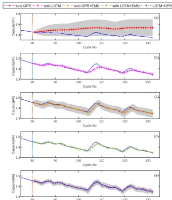
80 90 100 110 120 130 Cycle No. 1.4 1.6 1.8 Capacity[Ah]
solo GPR solo LSTM solo GPR+EMD solo LSTM+EMD LSTM+GPR
80 90 100 110 120 130 Cycle No. 1.3 1.4 1.5 Capacity[Ah] 80 90 100 110 120 130 Cycle No. 1.3 1.4 1.5 Capacity[Ah] 80 90 100 110 120 130 Cycle No. 1.3 1.4 1.5 Capacity[Ah] 80 90 100 110 120 130 Cycle No. 1.3 1.4 1.5 Capacity[Ah] (a) (b) (c) (d) (e)
Fig. 8. Capacity prediction results by using different data-driven models.(a) Solo GPR, (b) Solo LSTM, (c) Solo GPR+EMD, (d) Solo LSTM+EMD, (e)LSTM+GPR.
Fig. 8 and Table II illustrate the prediction results and accuracy indicators by using different models. Here all models are trained through using the previous 80 data from capacity degradation curve of B18. Then all the trained models are val-idated in its remaining cycles. It is worth noting that the solo GPR model cannot capture the trend of capacity degradation. The mean predictions from this solo model present a gradual upward trend with a wide confidence range, which shows little resemblance to the measured data. From Fig. 8 (b), it is observed that the whole degradation trend is well predicted, implying the satisfactory long-term capture performance of solo LSTM model. But several big mismatches appear in the regeneration points of around 105 cycles and 120 cycles, which means that the solo LSTM model may omit short-term fluctuations. In comparison, after EMD decomposition, it is obvious that all the prediction results become better. From Fig. 8 (c), the mean predictions of solo GPR+EMD become closer to the measured data but several delays occur
around the local regenerations. In Fig. 8 (d), by using the solo LSTM+EMD approach, mismatches between the pre-dictions and measured data decrease but no information on the prediction uncertainties are obtained. Through using the fusion way as illustrated in Eq. (4), our proposed LSTM+GPR model could provide both the predicted capacity values and the corresponding uncertainty quantification caused by the capacity regeneration phenomena. More details of this fusion way can be found in [19]. From. 8 (e), both long-term decline trend and short-term regeneration phenomena are well cap-tured as desired by using the combined LSTM+GPR model. Besides, the 95% confidence range in this case is distributed in a narrowest region, which indicates a small uncertainty for the predicted results. From Table II, the RMSE by using the LSTM+GPR model is just 0.0032, which is 98.2%, 34.7%, 11.1% and 5.9% less than the solo GPR, solo LSTM, solo GPR+EMD and solo GPR+LSTM, respectively. Accordingly, it can be concluded that the proposed LSTM+GPR model presents more efficient performance in predicting the long-term capacity decline trend whilst capturing the regeneration phenomena.
V. PREDICTION RESULTS AND DISCUSSIONS
In this section, to investigate the extrapolation performance of combined LSTM+GPR model, both 1-step and multi-step ahead capacity predictions are first conducted. Then the RUL prediction test is carried out for all battery cases. For 1-step and multi-step tests, due to page limitations, the prediction results of cells B05 and B06 are plotted but the accuracy indicators for all batteries are illustrated. Besides, to ensure enough information of capacity regeneration phenomena can be included in training process, first 80 data points (nearly 50/50 split) from capacity degradation curve are used as the training sets. Then the well-trained model is used to predict the future k-step capacity (k ≥ 1) in the remaining cycles without any retraining process. For our iterative prediction, the new estimation will be applied for the next prediction. Thus the corresponding uncertainty would be accumulated [33]. Considering this uncertainty propagation behaviour will lead to the estimation uncertainty bounds are getting larger with the cycle number increasing.
A. 1-step ahead capacity prediction TABLE III
ACCURACY INDICATORS OF1-STEP AHEAD PREDICTION. Battery No. B05 B06 B54 B55 C16 C38 RMSE (1-step) 0.0029 0.0037 0.0035 0.0038 0.0048 0.0042 Max error (1-step) 0.021 0.032 0.029 0.035 0.038 0.036
Maxcov(1-step) 0.027 0.016 0.021 0.025 0.034 0.031
Fig. 9 shows the 1-step ahead capacity prediction results of LSTM+GPR model for ’Case 1’ batteries. To evaluate the effectiveness of EMD, this test starts from a large regeneration process that occurs in the 87th cycle. From Fig. 9, it is evident that the trained model captures the evolution of both long-term capacity decline trends and regeneration phenomena for all
B05 80 90 100 110 120 130 140 150 160 170 Cycle No. 1.2 1.4 1.6 Capacity[Ah]
Test 1-step Ahead Prediction
B06 80 90 100 110 120 130 140 150 160 170 Cycle No. 1 1.2 1.4 1.6 Capacity[Ah] (a) (b)
Fig. 9. 1-step ahead prediction results. (a) B05, (b) B06.
batteries, as indicated by the satisfactory match between the predicted values and the actual data for the remaining points. Besides, all the 95% confidence bounds of these batteries are distributed in the narrow regions. According to the accuracy indicators as illustrated in Table III. The RMSE and the maximum error of the 1-step case are all within 0.0048 and 0.038 respectively, indicating that a high accuracy is attained by using our proposed model.
B. Multi-step ahead capacity prediction
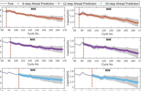
Next, to further investigate the extrapolation performance of proposed model for multi-step ahead prediction, tests based on various prediction horizons of 6, 12 and 24 steps are carried out. For these tests, inputs are obtained using 10 historical capacity data up to current cycle, and the prediction is conducted at the cyclek-step ahead of the current cycle.
TABLE IV
ACCURACY INDICATORS OF MULTI-STEP AHEAD PREDICTION Battery No. B05 B06 B54 B55 C16 C38 RMSE(6-step) 0.0038 0.0051 0.0041 0.0043 0.0054 0.0051 Max error(6-step) 0.027 0.035 0.032 0.037 0.042 0.041
Maxcov(6-step) 0.045 0.053 0.039 0.042 0.056 0.053 RMSE(12-step) 0.0036 0.0049 0.0045 0.0048 0.0059 0.0054 Max error(12-step) 0.023 0.034 0.035 0.036 0.048 0.046
Maxcov(12-step) 0.061 0.085 0.046 0.049 0.068 0.065 RMSE(24-step) 0.0041 0.0059 0.0056 0.0060 0.0068 0.0065 Max error(24-step) 0.025 0.037 0.042 0.047 0.055 0.052
Maxcov(24-step) 0.077 0.113 0.055 0.059 0.075 0.071
Fig. 10 presents the k-step ahead prediction results for ’Case 1’ batteries. It is obvious that several short-period mismatches occur in the multi-step prediction cases, which is mainly caused by the lack of priori information for the future large local fluctuations. However, the predicted capac-ities would gradually rematch the true test data again due to the effective information decomposition and the strong long-term capture ability of our proposed model. Interestingly, as the prediction step increases, the 95% confidence range will distribute in a wider region, indicating that the prediction uncertainty becomes larger. This is hardly surprising given that the long-step prediction generally contains much more uncertainty. Even so, the max cov value is still less than
TABLE V
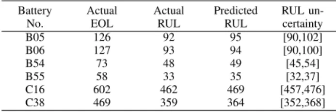
PERFORMANCE OFRULPREDICTIONS FOR ALL BATTERY CASES.
Battery No. Actual EOL Actual RUL Predicted RUL RUL un-certainty B05 126 92 95 [90,102] B06 127 93 94 [90,100] B54 73 48 49 [45,54] B55 58 33 35 [32,37] C16 602 462 469 [457,476] C38 469 359 364 [352,368]
±10% capacity range, which means that the prediction results are reliable. According to Table IV, the maximum RMSE for B05, B06, B54, B55, C16 and C38 become 0.0041, 0.0059, 0.0056, 0.0060, 0.0068 and 0.0065, which are 41.6%, 59.4%, 60.1%, 57.9%, 41.6% and 54.8% more than those of the 1-step case, respectively. However, all these values are less than 0.007, indicating that the satisfactory overall capacity predictions are also achieved for such cases. Therefore, the proposed LSTM+GPR model also presents good extrapolation performance for battery multi-step ahead prediction.
C. RUL prediction
According to the requirements of BHDS, predicting the future battery RUL as early as possible with a satisfactory accuracy level is more meaningful for battery real-world applications. In such a case, it is vital to predict battery RUL at an early cycle stage. In this subsection, in order to investigate the recursive prediction performance and the robustness of our proposed LSTM+GPR model, all batteries from NASA and CALCE are tested respectively. The corresponding quantitative results for all RUL prediction cases are illustrated in Table V. Here, the left and right bounds of uncertainty are defined by the first and last time instant when the obtained confidence range reaches the predefined battery EOL value, respectively. For ’Case 1’ batteries, to investigate the effects of various EOL values, the predefined EOLs of B05 and B06 are set as 75% and 66%, respectively. Fig. 11 illustrates the correspond-ing RUL prediction results. It is observed that for different batteries with different defined EOL values, the predicted ca-pacities present the similar trends with the real capacity curves. As illustrated in Table V, the actual EOL values of B05 and B06 are 126 and 127 cycles, respectively. When implementing the RUL prediction at the 34th cycle, the predicted RUL for B06 is 94, which is only 1 cycle (1.1%) later than the actual RUL. The predicted RUL for B05 is 3 cycles (3.3%) later than its actual RUL, respectively. Meanwhile, all the RUL uncertainty bounds of these predictions cover the real RUL values effectively.
Next, to verify the robustness of LSTM+GPR model, both ’Case 2’ batteries and ’Case 3’ batteries are used. For these batteries, the corresponding EOL values are all set as 80%. For ’Case 2’ batteries from NASA with low Tamb, the
corresponding RUL prediction results are plotted in Fig. 12. Although there are some mismatches exist especially in large fluctuation conditions, the whole capacity decline trends have been captured reliably. As illustrated in Table V, the capacity
B05 80 90 100 110 120 130 140 150 160 170 Cycle No. 1 1.2 1.4 1.6 Capacity[Ah]
Test 6-step Ahead Prediction 12-step Ahead Prediction 24-step Ahead Prediction B06 80 90 100 110 120 130 140 150 160 170 Cycle No. 1 1.2 1.4 1.6 Capacity[Ah] B05 80 90 100 110 120 130 140 150 160 170 Cycle No. 1 1.2 1.4 1.6 Capacity[Ah] B06 80 90 100 110 120 130 140 150 160 170 Cycle No. 1 1.2 1.4 1.6 Capacity[Ah] B05 80 90 100 110 120 130 140 150 160 170 Cycle No. 1 1.2 1.4 1.6 Capacity[Ah] B06 80 90 100 110 120 130 140 150 160 170 Cycle No. 1 1.2 1.4 1.6 Capacity[Ah]
Fig. 10. k-step ahead prediction results for ’Case 1’ batteries.
0 20 40 60 80 100 120 140 160 Cycle No. 1.2 1.4 1.6 1.8 2 Capacity[Ah] B05
Test Prediction RUL uncertainty
0 20 40 60 80 100 120 140 160 Cycle No. 1.2 1.4 1.6 1.8 2 Capacity[Ah] B06 (a) (b) 75% RUL 66% RUL
Fig. 11. RUL prediction results for ’Case 1’ batteries. (a) B05, (b) B06.
0 10 20 30 40 50 60 70 80 90 Cycle No. 0.8 0.9 1 1.1 1.2 Capacity[Ah] B54
Test Prediction RUL uncertainty
0 10 20 30 40 50 60 70 80 90 Cycle No. 1 1.1 1.2 1.3 1.4 Capacity[Ah] B55 (a) (b) 80% RUL 80% RUL
Fig. 12. RUL prediction results for ’Case 2’ batteries. (a) B54, (b) B55.
of B54 degrades below the EOL threshold at the 73rd cycle, thus the corresponding true RUL is 48. While the predicted RUL is 54, which is only 1 cycle (1.9%) delay. The RUL uncertainty bound here is [45, 54], covering the true RUL. For B55, the predicted RUL is 35, which is 2 cycles (5.3%) later
than the actual RUL. The corresponding uncertainty bound is [32, 37], which gets closer to the true RUL.
Fig. 13. RUL prediction results for ’Case 3’ batteries. (a) C16, (b) C38.
Fig. 13 illustrates the RUL prediction results for ’Case 3’ batteries from CALCE with long capacity aging cycle. Here the actual RULs of C16 and C38 are 602 and 409, respectively. Even so, it is observed that the overall trends of both C16 and C38 have been well captured by LSTM+GPR model. The predicted RULs for C16 and C38 become 468 and 363, which are 7 cycles and 5 cycles later than their true RULs, respectively. In comparison with NASA data with less than 200 cycles, these increased delays are reasonable due to the accumulated prediction errors in long iteration process. However, the corresponding uncertainty bounds still cover true RULs (here is [457, 476] for C16 and [352, 368] for C38), indicating that the uncertainty managements in such cases are still reliable. It can be observed that for the above experiments, the predicted capacity trajectories all present smooth fluctuations. These predicted fluctuations are reasonable due to the fact that after EMD decomposition, these
information within the IMFs can be extracted and learned. More information regarding these phenomena can be found in [19]. Therefore, based on the above experimental analyses, we can conclude that by training the developed model at early cycle conditions, the efficient RUL prediction can be achieved with acceptable accuracy and good robustness for different battery health diagnosis.
D. Further Discussions
This article focuses on the development of a data-driven approach to achieve reliable battery future capacities and RUL prediction with uncertainty quantification for Li-ion batteries by capturing both long-term dynamics and local regenerations directly. Due to the calculation environment is Matlab 2018, the computational complexity is relatively low through using the RNN and GPR toolboxes (here the maximum training time is within 5s). Indeed, developing a sufficiently accurate and robust data-driven model including uncertainty management is an open research problem. Even though the capacity long-term dependence and the prediction confidence level can be simultaneously considered by the proposed framework, the corresponding performance highly depends on the form of data and quality of test experiments, which is a common problem for pure data-driven applications.
VI. CONCLUSION
An innovative data-driven approach has been proposed to enable accurate health prognosis with reliable uncertainty quantification for Li-ion batteries. This is the first known application of combining the superiorities of LSTM (recurrent links and multiple gate) and GPR (non-parametric and prob-abilistic) for future capacities and RUL prediction. Through detailed result analyses and comparisons, some conclusions are obtained as:
1) The long-term capacity degradation dynamics is correctly captured by the LSTM, while the uncertainties caused by capacity regenerations can be well expressed through using GPR, further resulting in an improved prediction results.
2) In comparison with the solo GPR, solo LSTM, solo GPR+EMD and solo LSTM+EMD models, the proposed LSTM+GPR model outperforms other counterparts with just 0.0032 RMSE and 0.6% maximum error, respectively.
3) For both 1-step and multi-step ahead predictions, the LSTM+GPR model achieve satisfactory extrapolation perfor-mance with less than 1.8% maximum error for all cases.
4) Even starting the RUL predictions at the early cycle stages, LSTM+GPR model also presents the good general-ization ability and reliable uncertainty management for the applications of all ’Case 1’, ’Case 2’, and ’Case 3’ batteries. Future work includes effective feature extractions after collecting valuable data for the second stage trend of Li-ion batteries, and the improvement of our data-driven approach for the battery ’knee point’ prediction.
REFERENCES
[1] Z. Wei, J. Zhao, R. Xiong, G. Dong, J. Pou, and K. J. Tseng, “Online estimation of power capacity with noise effect attenuation for lithium-ion battery,”IEEE Transactions on Industrial Electronics, vol. 66, no. 7, pp. 5724–5735, 2018.
[2] M. Berecibar, I. Gandiaga, I. Villarreal, N. Omar, J. Van Mierlo, and P. Van den Bossche, “Critical review of state of health estimation meth-ods of li-ion batteries for real applications,”Renewable and Sustainable Energy Reviews, vol. 56, pp. 572–587, 2016.
[3] C. Lyu, Q. Lai, T. Ge, H. Yu, L. Wang, and N. Ma, “A lead-acid battery’s remaining useful life prediction by using electrochemical model in the particle filtering framework,”Energy, vol. 120, pp. 975–984, 2017. [4] G. Dong, Z. Chen, J. Wei, and Q. Ling, “Battery health prognosis using
brownian motion modeling and particle filtering,”IEEE Transactions on Industrial Electronics, 2018.
[5] Y. Chang, H. Fang, and Y. Zhang, “A new hybrid method for the prediction of the remaining useful life of a lithium-ion battery,”Applied Energy, vol. 206, pp. 1564–1578, 2017.
[6] D. Wang, F. Yang, K.-L. Tsui, Q. Zhou, and S. J. Bae, “Remaining useful life prediction of lithium-ion batteries based on spherical cubature particle filter,”IEEE Transactions on Instrumentation and Measurement, vol. 65, no. 6, pp. 1282–1291, 2016.
[7] L. Zhang, Z. Mu, and C. Sun, “Remaining useful life prediction for lithium-ion batteries based on exponential model and particle filter,” IEEE Access, vol. 6, pp. 17 729–17 740, 2018.
[8] K. Liu, K. Li, Q. Peng, and C. Zhang, “A brief review on key technologies in the battery management system of electric vehicles,” Frontiers of mechanical engineering, vol. 14, no. 1, pp. 47–64, 2019. [9] C. Zhang, Y. He, L. Yuan, and S. Xiang, “Capacity prognostics of
lithium-ion batteries using emd denoising and multiple kernel rvm,” IEEE Access, vol. 5, pp. 12 061–12 070, 2017.
[10] J. Wei, G. Dong, and Z. Chen, “Remaining useful life prediction and state of health diagnosis for lithium-ion batteries using particle filter and support vector regression,”IEEE Transactions on Industrial Electronics, vol. 65, no. 7, pp. 5634–5643, 2018.
[11] J. Wu, C. Zhang, and Z. Chen, “An online method for lithium-ion battery remaining useful life estimation using importance sampling and neural networks,”Applied energy, vol. 173, pp. 134–140, 2016.
[12] H. Dai, G. Zhao, M. Lin, J. Wu, and G. Zheng, “A novel estima-tion method for the state of health of lithium-ion battery using prior knowledge-based neural network and markov chain,”IEEE Transactions on Industrial Electronics, 2018.
[13] Y. Song, D. Liu, C. Yang, and Y. Peng, “Data-driven hybrid remain-ing useful life estimation approach for spacecraft lithium-ion battery,” Microelectronics Reliability, vol. 75, pp. 142–153, 2017.
[14] S. S. Ng, Y. Xing, and K. L. Tsui, “A naive bayes model for robust remaining useful life prediction of lithium-ion battery,”Applied Energy, vol. 118, pp. 114–123, 2014.
[15] X. Hu, J. Jiang, D. Cao, and B. Egardt, “Battery health prognosis for electric vehicles using sample entropy and sparse bayesian predictive modeling,”IEEE Transactions on Industrial Electronics, vol. 63, no. 4, pp. 2645–2656, 2016.
[16] C. Hu, H. Ye, G. Jain, and C. Schmidt, “Remaining useful life assess-ment of lithium-ion batteries in implantable medical devices,”Journal of Power Sources, vol. 375, pp. 118–130, 2018.
[17] Y. Zhang, R. Xiong, H. He, and M. Pecht, “Lithium-ion battery remaining useful life prediction with box-cox transformation and monte carlo simulation,”IEEE Transactions on Industrial Electronics, 2018. [18] B. E. Olivares, M. A. C. Munoz, M. E. Orchard, and J. F. Silva,
“Particle-filtering-based prognosis framework for energy storage devices with a statistical characterization of state-of-health regeneration phenomena,” IEEE Transactions on Instrumentation and Measurement, vol. 62, no. 2, pp. 364–376, 2013.
[19] Y. Zhou and M. Huang, “Lithium-ion batteries remaining useful life prediction based on a mixture of empirical mode decomposition and arima model,”Microelectronics Reliability, vol. 65, pp. 265–273, 2016. [20] Y. Xing, E. W. Ma, K.-L. Tsui, and M. Pecht, “An ensemble model for predicting the remaining useful performance of lithium-ion batteries,” Microelectronics Reliability, vol. 53, no. 6, pp. 811–820, 2013. [21] R. R. Richardson, M. A. Osborne, and D. A. Howey, “Gaussian process
regression for forecasting battery state of health,” Journal of Power Sources, vol. 357, pp. 209–219, 2017.
[22] J. Chung, C. Gulcehre, K. Cho, and Y. Bengio, “Empirical evaluation of gated recurrent neural networks on sequence modeling,”arXiv preprint arXiv:1412.3555, 2014.
[23] G.-W. You, S. Park, and D. Oh, “Diagnosis of electric vehicle batteries using recurrent neural networks,” IEEE Transactions on Industrial Electronics, vol. 64, no. 6, pp. 4885–4893, 2017.
[24] Y. Zhang, R. Xiong, H. He, and M. Pecht, “Long short-term memory recurrent neural network for remaining useful life prediction of lithium-ion batteries,”IEEE Transactions on Vehicular Technology, 2018.
[25] G. O. Sahinoglu, M. Pajovic, Z. Sahinoglu, Y. Wang, P. V. Orlik, and T. Wada, “Battery state-of-charge estimation based on regular/recurrent gaussian process regression,”IEEE Transactions on Industrial Electron-ics, vol. 65, no. 5, pp. 4311–4321, 2018.
[26] D. Yang, X. Zhang, R. Pan, Y. Wang, and Z. Chen, “A novel gaussian process regression model for state-of-health estimation of lithium-ion battery using charging curve,”Journal of Power Sources, vol. 384, pp. 387–395, 2018.
[27] B. Saha and K. Goebel, “Modeling li-ion battery capacity depletion in a particle filtering framework,” inProceedings of the annual conference of the prognostics and health management society, pp. 2909–2924, 2009. [28] R. R. Richardson, C. R. Birkl, M. A. Osborne, and D. Howey, “Gaussian
process regression for in-situ capacity estimation of lithium-ion batter-ies,”IEEE Transactions on Industrial Informatics, 2018.
[29] J. Han and M. van der Baan, “Empirical mode decomposition for seismic time-frequency analysis,”Geophysics, vol. 78, no. 2, pp. O9–O19, 2013. [30] C. K. Williams and C. E. Rasmussen, “Gaussian processes for machine
learning,”the MIT Press, vol. 2, no. 3, p. 4, 2006.
[31] M. Kl¨as and A. M. Vollmer, “Uncertainty in machine learning appli-cations: A practice-driven classification of uncertainty,” inInternational Conference on Computer Safety, Reliability, and Security, pp. 431–438. Springer, 2018.
[32] X. Tang, C. Zou, K. Yao, G. Chen, B. Liu, Z. He, and F. Gao, “A fast estimation algorithm for lithium-ion battery state of health,”Journal of Power Sources, vol. 396, pp. 453–458, 2018.
[33] K. Liu, X. Hu, Z. Wei, Y. Li, and Y. Jiang, “Modified gaussian process regression models for cyclic capacity prediction of lithium-ion batteries,”IEEE Transactions on Transportation Electrification, vol. 5, DOI 10.1109/TTE.2019.2944802, no. 4, pp. 1225–1236, Dec. 2019.
Kailong Liu(M’18) is a Senior Research Fellow in the Warwick Manufacturing Group, University of Warwick, United Kingdom. He received the B.Eng. degree in electrical engineering and the M.Sc. degree in control theory and control en-gineering from Shanghai University, China, and the Ph.D. degree in electrical engineering from the Energy, Power and Intelligent Control group, Queen’s University Belfast, United Kingdom, in 2011, 2014, and 2018, respectively.
He was a Visiting Student Researcher at the Tsinghua University and the North China Electric Power University, China, in 2016. His research interests include modeling, optimization and control with applications to electrical/hybrid vehicles, energy stor-age, as well as battery manufacture and management.
Dr. Liu was the student chair of IEEE QUB student branch and a re-cipient of awards such as EPSRC Scholarship, Santander International Scholarship, and QUB ESM International Scholarship.
Yunlong Shang(S’14-M’18) received the B.S. degree in automation from Hefei University of Technology, China, in 2008 and the Ph.D. degree in control theory and control engineering from Shandong University, China, in 2017.
In 2019, he joined Shandong University, where he is currently a full Professor and Qilu Youth Talent Scholar with the School of Control Science and Engineering. Between September 2015 and October 2017, he conducted scien-tific research as a joint Ph.D. student with the Department of Electrical and Computer Engineering, San Diego State University, San Diego, CA, USA, where between December 2017 and January 2019, he was a Postdoctoral Research Fellow. His current research interests include battery balancing, battery modeling and states estimation, self-heating for low-temperature batteries, and design of battery management systems (BMS). In 2018, Prof. Shang wined the excellent doctoral dissertation award of Chinese Association of Automation (CAA).
Quan Ouyang was born in 1991 in Hubei Province, China. He received the B. S. degree in Automation from Huazhong University of Sci-ence and Technology, China, in 2013, and the Ph.D. degree in Control Science and Engineer-ing from Zhejiang University, China, in 2018, respectively. He is currently a lecturer in the College of Automation engineering, Nanjing Uni-versity of Aeronautics and Astronautics, Nanjing, Jiangsu, China. His research interests mainly include battery management, modeling and con-trol of Fuel Cell systems, and nonlinear concon-trol.
Dhammika Widanalageis an Assistant Profes-sor in modelling and energy storage at WMG, Warwick University and was the recipient of the WMG Early Career Researcher of the Year award in 2016. His research is in system iden-tification theory, applied across several applica-tions including batteries.
He leads the battery modelling research in the department and recently secured funding to lead the modelling activity as a PI (for WMG) on the Faraday Multiscale Modelling project, as a Co-I on the EPSRC Prosperity Partnership with Jaguar Land Rover and a PI and Co-I on four Innovate UK projects (PI and three Co-I). He is a member of the European Materials Modelling Community Interoperabil-ity and Repository Advisory Group (EMMC-IRAG) and supported the compilation of the Materials modelling-Terminology, Classification and Metadata document which is now publicly available to increase the use of material modelling with industrial end-users.