Conjectures on an algorithm for convex parametric quadratic programs

Conjectures on an algorithm for convex parametric quadratic programs J. Spjøtvold, E. C. Kerrigan, C. N. Jones,

T. A. Johansen, P. Tøndel CUED/F-INFENG/TR.496

Conjectures on an algorithm for convex parametric

quadratic programs

Jørgen Spjøtvold

Eric C. Kerrigan

Colin N. Jones

Tor A. Johansen

Petter Tøndel

a_{Department of Engineering Cybernetics,}

Norwegian University of Science and Technology, N-7491 Trondheim, Norway.

b_{Department of Engineering,}

University of Cambridge, Trumpington Street, Cambridge CB2 1PZ, United Kingdom.

Abstract

An algorithm for convex parametric QPs is studied. The algorithm explores the parameter space by stepping a sufficiently small distance over the facets of each critical region and thereby identifying the neighboring regions. Some conjectures concerning this algorithm and the structure of the solution of a parametric QP are presented.

Key words: Parametric programming, Quadratic programming, Linear programming.

1 Introduction

Algorithms for solving parametric quadratic programs [2,6] and parametric linear programs [3] have been developed recently. The algorithms proposed in [2] and [3] introduce artificial cuts in the parameter space in the search for the solution, while in [6] an algorithm based on considering all faces of the constraint polyhedron is presented. In [1] and [4] the authors propose a method for exploring the parameter space, which is conceptually more efficient than in [2,3,6]; by stepping a suffi-1 _{Technical Report CUED/F-INFENG/TR.496, Department of Engineering, University of} Cambridge, UK, 28 October 2004.

ciently small distance over the boundary of a so-called critical region1 and solving an LP/QP for the resulting parameter, a new critical region is defined. This proce-dure looks promising, but seems to implicitly rely on the assumption that the facets of neighboring regions satisfy a certain property, namely that their intersection is a facet of both regions. We will refer to this as the facet-to-facet property. It seems intuitively correct that if the facet-to-facet property holds, an algorithm based on stepping over the facets will explore the whole parameter space; however, to the best of our knowledge, a proof that the critical regions satisfy the facet-to-facet property has not been presented in the literature.

In [7,8] the authors propose a method in which each facet of the critical region is examined and depending on whether the facet ensures feasibility or optimality, the active set in the neighboring is found by adding or removing a constraint from the current active set. This algorithm relies on the LICQ assumption and must, in some cases, also step anǫ-distance over a facet to determine the active set in the adjacent region.

The algorithms presented in [1,2,4,6] are applied to parametric QPs with a positive definite Hessian. We will, in addition to the strictly convex problem, consider the more general formulation given in [8] where the Hessian is allowed to be positive semidefinite, the objective function can be linear and/or include a bilinear term. We state some conjectures that need to be proven before an algorithm based on stepping over the facets will guarantee that the critical regions cover the part of the parameter space that renders the optimization problem feasible.

2 Notation, definitions, problem setup and assumptions

If A is a matrix, thenAi denotes the ith row of A andAI denotes the rows of A

corresponding to the index setI.

Recall that the set of affine combinations of points in a set S ⊂ Rn _{is called the}

affine hull ofS. The dimension of a setS ⊂_Rn_{is the dimension of the affine hull}

ofS, and is denoteddim(S); ifdim(S) = n, thenS is said to be full-dimensional (note that a set is full-dimensional if and only if its interior is non-empty). A poly-hedron is the intersection of a finite number of closed halfspaces. F is a face of the polyhedronP ⊂ _Rn_{if there exists a hyperplane {z ∈}

Rn | aT_{z = b}, wherea ∈}

Rn_{, b ∈ R, such that F = P ∩ {z ∈ R}n _{| a}T_{z = b} and a}T_{z ≤ b, ∀z ∈ P.}

Given an s-dimensional polyhedron P ⊂ _Rn_{, where s ≤ n, the facets of P are}

the(s−1)-dimensional faces ofP.

1 _{A critical region is the set of parameters for which some fixed set of constraints are} fulfilled with equality at all solutions of an optimization problem.

Consider the following parametric quadratic program (QP): J∗(θ), min x∈_Rn f(x, θ), 1 2x T_Hx+θT_FT_x+cT_{x|Ax≤b+Sθ,} (1)

whereθ ∈ _Rs _{is a parameter of the optimization problem, and the vector x ∈}

Rn

is to be optimized for all values of θ ∈ Θ, where Θ ⊆ Rs _{is some polyhedral}

set. Moreover, H = HT _∈

Rn×n, F ∈ _Rn×s_{, A ∈}

Rq×n, b ∈ _Rq×₁

, S ∈ _Rq×s

andc∈_Rn×1_{. If, in additionH≥0orH >0, then the parametric QP is convex or} strictly convex, respectively. IfH = 0, then we refer to (1) as a parametric linear program (LP).

The set of parameters for which the minimum in (1) exists, denotedΘ∗

, is generally a subset ofΘ. IfΘ∗

is a strict subset ofΘ, the set of parameters for which we seek the solution is redefined, i.e.Θ,Θ∗. IfΘ∗ is lower-dimensional, problem (1) can be re-parameterized [3] and one can consider a reduced parameter vector θ¯such thatΘ¯∗

is full-dimensional. Consequently, in the sequel we will make the following assumption:

Assumption 1 The set of admissible parametersΘis full-dimensional. We also as-sume that for allθ∈Θ, the set of feasible pointsX(θ),{x∈Rn_|Ax≤b+Sθ}

is non-empty and the minimum in (1) exists.

Definition 1 (Active set) Letx be a feasible point of (1) for a givenθ. We define the active constraints as the constraints that fulfill Aix−bi −Siθ = 0, and the

inactive constraints as those that fulfillAix−bi−Siθ <0. The active setA(x, θ)

is the set of indices of the active constraints, that is,

A(x, θ),{i∈ {1, . . . , q} |Aix−bi−Siθ = 0}.

Moreover, letN(x, θ)denote the set of inactive constraints, that is, N(x, θ),{1, . . . , q}\A(x, θ).

Definition 2 (Solution set) The set of solutions to (1) for a givenθis defined as

X∗(θ),{x∈Rn |Ax≤b+Sθ, f(x, θ) = J∗(θ)}.

Definition 3 (Optimal active set) Letθbe given, then the optimal active setA∗

(θ) is the set of constraints that are active for allx∈X∗(θ), that is

A∗(θ),{i|i∈ A(x, θ), ∀x∈X∗(θ)}= \ x∈X∗_(θ) A(x, θ). LetN∗ (θ),{1, . . . , q}\A∗ (θ).

Definition 4 (Critical region) Given an optimal active setA∗

, the critical regionΘA∗ is the set of parameters for which the optimal active set remains unchanged, that

is,

ΘA∗ ,{θ∈Θ| A

∗

(θ) =A∗}. (2)

Definition 5 (LICQ) For an active set A, we say that the linear independence constraint qualification (LICQ) holds if the set of active constraint gradients are linearly independent, i.e.AAhas full row rank.

3 An algorithm for exploring the parameter space

We will consider the performance of a conceptual algorithm based on stepping a small distance over all facets of a critical region and identifying the optimal active set in all (or some) of the neighboring regions. In [1,4] this algorithm is utilized to solve parametric QPs with a positive definite Hessian. The focal point of this document is to establish the properties (1) must fulfill in order to ensure that the al-gorithm is well behaved. Before the alal-gorithm is presented, the following properties for the parametric QP (1) should be noted [2,3,7]:

• Critical regions are convex and their closures are polyhedral. • Θis convex and polyhedral.

• The optimal active set is unique for allθ ∈Θ.

• Since the optimal active set is unique, critical regions cannot intersect. However, though the intersection of any two full-dimensional critical regions is empty, the intersection of their closures may be non-empty.

• Since the set of admissible parametersΘis assumed to be full-dimensional and the number of optimal active sets is finite, there exists a finite number of full-dimensional critical regions such that the union of their closures is equal toΘ. In the light of the properties above the goal of the algorithm considered here is to identify only the full-dimensional critical regions. Since we are only identifying the full-dimensional regions, we will, in conformity with [1–4,6–8], only work with the closure of each critical region instead of the region itself. In the sequel, we will therefore abbreviate closure of the/a full-dimensional critical region to critical region.

The procedure for exploring the parameter space is given in Algorithm 1. The out-put of Algorithm 1 is a collectionRof closures of full-dimensional critical regions for (1). From this point on, we will letK denote the number of sets inR andRk

refer to thekth_{set inR.}

Consider now the question: Under which assumptions on the problem data of (1) will Algorithm 1 guarantee thatSK

k=1Rk = Θ? For this purpose, we introduce the

Algorithm 1 Exploring the parameter space.

Input: A parameterθin the interior of a critical region. Output: Set of critical regionsR.

1: IdentifyA∗

(θ).

2: Construct the irredundant representation of the critical regioncl(ΘA∗_(θ)) ={θ |

Ciθ ≤di, i= 1, . . . , m}.

3: Addcl(ΘA∗_(θ))to the setRof discovered regions.

4: for each facetiin the description ofcl(ΘA∗_(θ))do

5: Letθ0 = ˆθ+ǫCi, whereθˆis such thatCiθˆ=di andCjθ < dˆ j, for allj 6=i,

and ǫ > 0 is a sufficiently small scalar such that the resulting parameter point θ₀ is in the interior of a neighboring, critical region ΘA∗_(θ0) in the

sense thatcl(ΘA∗_(θ))∩cl(ΘA∗_(θ0))6=∅.

6: If θ0 is not in a previously discovered critical region, make a recursive call to Algorithm 1 withθ₀ as the new parameter.

7: end for

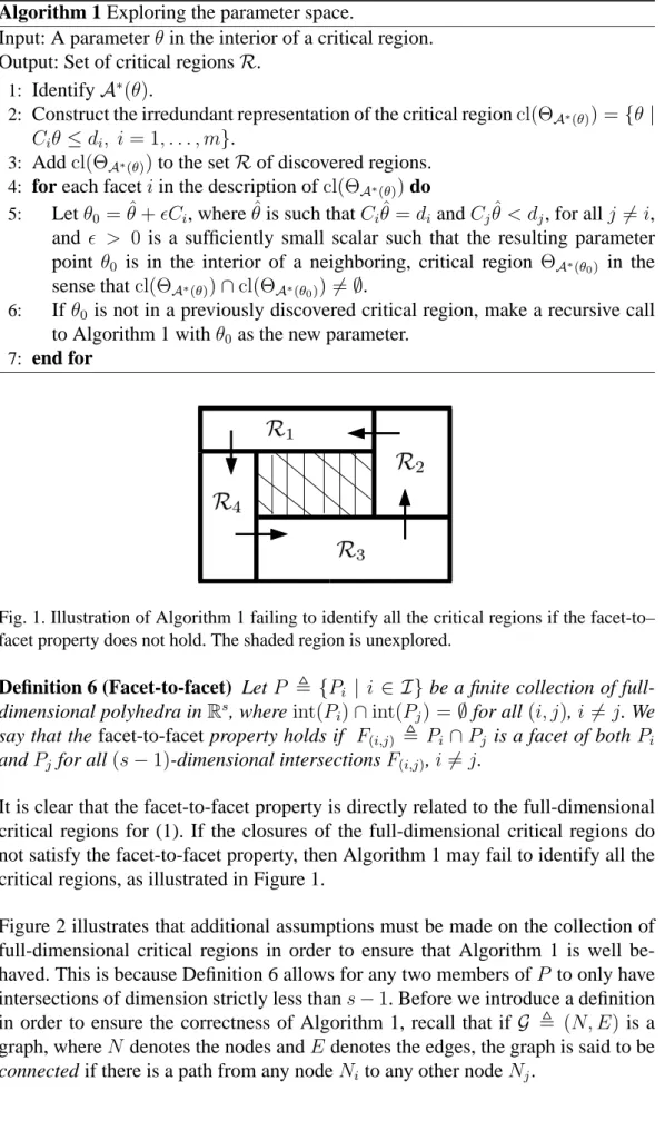
Fig. 1. Illustration of Algorithm 1 failing to identify all the critical regions if the facet-to– facet property does not hold. The shaded region is unexplored.

Definition 6 (Facet-to-facet) Let P , {Pi | i ∈ I}be a finite collection of

full-dimensional polyhedra in_Rs, whereint(Pi)∩int(Pj) = ∅for all(i, j),i 6=j. We

say that the facet-to-facet property holds if F₍i,j) , Pi∩Pj is a facet of both Pi

andPj for all(s−1)-dimensional intersectionsF(i,j),i6=j.

It is clear that the facet-to-facet property is directly related to the full-dimensional critical regions for (1). If the closures of the full-dimensional critical regions do not satisfy the facet-to-facet property, then Algorithm 1 may fail to identify all the critical regions, as illustrated in Figure 1.

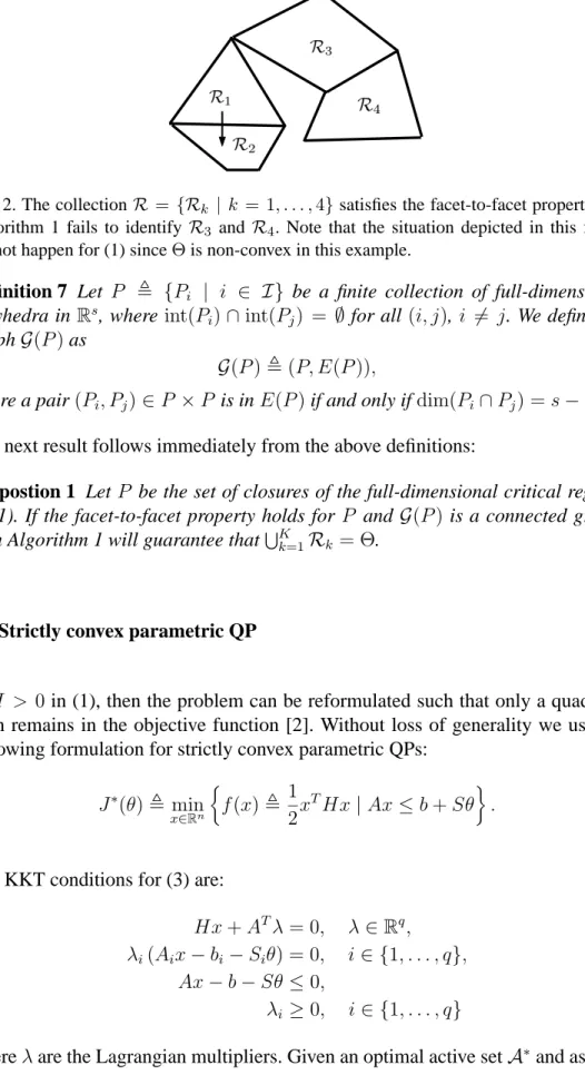
Figure 2 illustrates that additional assumptions must be made on the collection of full-dimensional critical regions in order to ensure that Algorithm 1 is well be-haved. This is because Definition 6 allows for any two members ofP to only have intersections of dimension strictly less thans−1. Before we introduce a definition in order to ensure the correctness of Algorithm 1, recall that if G _, (N, E) is a graph, whereN denotes the nodes andEdenotes the edges, the graph is said to be connected if there is a path from any nodeNi to any other nodeNj.

Fig. 2. The collectionR = {Rk | k = 1, . . . ,4}satisfies the facet-to-facet property, but

Algorithm 1 fails to identify R3 and R4. Note that the situation depicted in this figure cannot happen for (1) sinceΘis non-convex in this example.

Definition 7 Let P , {Pi | i ∈ I} be a finite collection of full-dimensional

polyhedra in _Rs_{, where int(P}

i)∩int(Pj) = ∅for all (i, j), i 6= j. We define the

graphG(P)as

G(P),(P, E(P)),

where a pair(Pi, Pj)∈P ×P is inE(P)if and only ifdim(Pi∩Pj) =s−1.

The next result follows immediately from the above definitions:

Propostion 1 LetP be the set of closures of the full-dimensional critical regions of (1). If the facet-to-facet property holds for P and G(P)is a connected graph, then Algorithm 1 will guarantee thatSK

k=1Rk = Θ.

4 Strictly convex parametric QP

IfH > 0in (1), then the problem can be reformulated such that only a quadratic term remains in the objective function [2]. Without loss of generality we use the following formulation for strictly convex parametric QPs:

J∗(θ), min x∈_Rn f(x), 1 2x T_Hx|Ax≤b +Sθ . (3)

The KKT conditions for (3) are:

Hx+ATλ = 0, λ∈_Rq_,

(4a)

λi(Aix−bi−Siθ) = 0, i∈ {1, . . . , q}, (4b)

Ax−b−Sθ ≤0, (4c)

λi ≥0, i∈ {1, . . . , q} (4d)

whereλare the Lagrangian multipliers. Given an optimal active setA∗

assum-ing that LICQ holds, the KKT conditions can be manipulated to obtain [2] x∗ =−H−1ATA∗λA∗, (5a) λA∗ =−(AA∗H −1_AT A∗) −1_(b A∗+SA∗θ), (5b)

and the closure of the critical region becomes cl(ΘA∗) ={θ ∈Θ|AN∗x

∗

(θ)≤bN∗+SN∗θ, λA∗(θ)≥0}. (6) Conjecture 1 LetH > 0in (3). If LICQ holds forAA∗ for all optimal active sets that define full-dimensional critical regions for (3), then Algorithm 1 guarantees thatSK

k=1Rk= Θ.

4.1 Non-unique Lagrangian multipliers

If LICQ is violated forAA∗then one cannot defineλA∗by (5b). In [2] this is solved simply by selecting a subset of the active constraints such that the resulting system of equalities has full rank. The region is then characterized using (5a) and (5b) on the reduced system. The resulting region is not a critical region in the sense of Definition 4; that is,ΘA∗is partitioned into subregions.

Consider the question: Will Algorithm 1 guarantee that SK

k=1Rk = Θ for (3) if

regions are constructed by using a reduced active set whenever LICQ is violated? Example 1 Consider the following problem [8]:

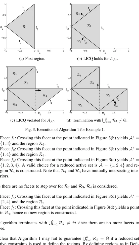
J∗(θ),min x∈_R3 1 2x T_{x |x∈X(θ), θ∈Θ,} X(θ),                    x∈_R3 x₁ −x₃ ≤ −1 +θ₁ −x₁ −x₃ ≤ −1 −θ₁ x₂ −x₃ ≤ −1 −θ₂ −x₂ −x₃ ≤ −1 +θ₂                    ,Θ,      θ∈_R2 −1 ≤ θ₁ ≤ 1 −1 ≤ θ₂ ≤ 1      . Letθ0 = −0.5 −0.2 T , which results in A∗

(θ0) = {1,2,3,4} and LICQ is vio-lated for AA∗. If the method in [2] is used, one may choose A = {1,3,4}as the reduced active set, and the resulting region is depicted in Figure 3(a). We iterate Algorithm 1 for the closure R1 of the first critical region. Note that the order in which the facets are stepped over differs slightly from Algorithm 1, however, the concept is the same.

−1 −0.5 0 0.5 1 −1 −0.5 0 0.5 1 θ₁ θ₂ f 1 f 2 f 3

(a) First region.

−1 −0.5 0 0.5 1 −1 −0.5 0 0.5 1 θ₁ θ₂ f 1 f 2 f 3

(b) LICQ holds forAA∗.

−1 −0.5 0 0.5 1 −1 −0.5 0 0.5 1 θ₁ θ₂ f 3 f₅ f₄

(c) LICQ violated forAA∗.

−1 −0.5 0 0.5 1 −1 −0.5 0 0.5 1 θ₁ θ₂ f 5 f 4 (d) Termination withS5 k=1Rk 6= Θ.

Fig. 3. Execution of Algorithm 1 for Example 1.

(1) Facetf1: Crossing this facet at the point indicated in Figure 3(b) yieldsA∗ = {1,3}and the regionR2.

(2) Facetf₂: Crossing this facet at the point indicated in Figure 3(b) yieldsA∗

= {1,4}and the regionR3.

(3) Facetf3: Crossing this facet at the point indicated in Figure 3(c) yieldsA∗ = {1,2,3,4}. A valid choice for a reduced active set isA = {1,2,4} and re-gionR4is constructed. Note thatR1 andR4 have mutually intersecting inte-riors.

Since there are no facets to step over forR2andR3,R4 is considered.

(1) Facetf₄: Crossing this facet at the point indicated in Figure 3(d) yieldsA∗

= {2,4}and the regionR5.

(2) Facetf5: Crossing this facet at the point indicated in Figure 3(d) yields a point inR1, hence no new region is constructed.

The algorithm terminates with S5

k=1Rk 6= Θ since there are no more facets to

explore.

It is clear that Algorithm 1 may fail to guarantee SK

k=1Rk = Θ if a reduced set

Defi-0 0.5 1 1.5 2 −2 −1.5 −1 −0.5 0 θ₁ θ₂

Fig. 4. Full-dimensional critical regions for Example 2.

nition 4, neighboring regions cannot have mutually intersecting interiors. Thus, we state the following conjecture:

Conjecture 2 Let H > 0in (3). If critical regions are defined as in Definition 4, then Algorithm 1 will guarantee thatSK

k=1Rk = Θfor (3).

5 Convex parametric QP

Consider (1) and letH =HT _{≥ 0. Note thatH ≥0includes the case whereH =}

0. An example will illustrate that the facet-to-facet property may not hold for this problem class. Example 2 J∗(θ),min x∈_R2{θ2x1+θ1x2 |x∈X(θ), θ∈Θ}, X(θ),                    x∈R2 x₁ −x₂ ≤ 0 −x₁ −x₂ ≤ 0 −x₂ ≤ −1−θ₂ x₂ ≤ 5                    ,Θ,      θ∈R2 0 ≤ θ₁ ≤ 2 −2 ≤ θ₂ ≤ 0      .

The unique solution for this problem is depicted in Figure 4 and the active sets and optimizers are given in Table 1.

The solution to the problem for some fixed parameter vectors are depicted in Fig-ures 5(a)–5(d). It is clear that by stepping over the diagonal facet ofR1, two re-gions can be defined, depending on the value of θˆ. Readers that are unfamiliar with the normal cone optimality condition are referred to the appendix. It should

Table 1

Active sets and optimizers for Example (2).

R1 R2 R3 A∗(θ) {1,4} {1,2} {1,3} x∗(θ) x ∗ 1(θ) = 5 x∗₂(θ) = 5 x∗₁(θ) = 0 x∗₂(θ) = 0 x∗₁(θ) =θ2+ 1 x∗₂(θ) =θ2+ 1 (a)θ1 = 0.5, θ2 =−0.4 (b) θ1= 0.5, θ2 =−0.6 (c) θ1= 1.5, θ2=−1.6 (d) θ1= 1.5, θ2=−1.4 Fig. 5. Illustration of Example 2.

be noted that the violation of the facet-to-facet property can just as easily occur ifH 6= 0. Adding an additional variablex₃ to the problem and modifying the cost to 1₂x2₃+θ₂x₁+θ₁x₂ yields the same collection of full-dimensional critical regions.

The violation of the facet-to-facet property seems to be a consequence of the bi-linear term in the objective function in combination with parameters on the right hand side of the constraints. In Example 2 the solution changes with the param-eter in a discontinuous fashion due to the presence of the bilinear term, and as a result the facet-to-facet property is violated. In the absence of a bilinear term, the point-to-set map X∗(·) is continuous and the authors have not been able to find an example for which the facet-to-facet property is violated. On the other hand, ifS = 0, butF 6= 0, then the solution may change in a discontinuous fashion, but then we are minimizing over a fixed polyhedron and it seems reasonable that the facet-to-facet property holds. We therefore state the following conjecture:

Conjecture 3 Let H ≥ 0in (1). If critical regions are defined as in Definition 4, then Algorithm 1 will guarantee thatSK

k=1Rk = Θfor (1) if eitherF = 0orS = 0.

6 Conclusions

We presented some conjectures that need to be proven before an algorithm for parametric QPs based on stepping over each facet of a critical region will guarantee that the whole parameter space is explored. An example showed that one needs to ensure that critical regions are uniquely defined for each parameter vector. A simple example also illustrated that the facet-to-facet property does not hold for a special class of parametric QPs. Current research is devoted to proving the conjectures.

References

[1] M. Baoti´c. An efficient algorithm for multi-parametric quadratic programming. Technical Report AUT02-05, ETH Z¨urich, Institut f¨ur Automatik, Physikstrasse 3, CH-8092, Switzerland, 2002.

[2] A. Bemporad, M. Morari, V. Dua, and E. N. Pistikopoulos. The explicit linear quadratic regulator for constrained systems. Automatica, 38(1):3–20, 2002.

[3] F. Borrelli, A. Bemporad, and M. Morari. A geometric algorithm for multi-parametric linear programming. Journal of Optimization Theory and Applications, 118(3):515– 540, 2003.

[4] P. Grieder, F. Borrelli, F. Torrisi, and M. Morari. Computation of the constrained infinite time linear quadratic regulator. Automatica, 40:701–708, 2004.

[5] J. Nocedal and S. J. Wright. Numerical Optimization. Springer, New York, USA, 1999.

[6] M. M. Seron, G. C. Goodwin, and J. A. De Don´a. Geometry of model predictive control for constrained linear systems. Technical Report EE0031, Department of Electrical and

Computer Engineering, The University of Newcastle, Callaghan, NSW 2308, Australia, September 2000.

[7] P. Tøndel, T. A. Johansen, and A. Bemporad. An algorithm for multi-parametric quadratic programming and explicit MPC solutions. Automatica, 39(3):489–497, 2003.

[8] P. Tøndel, T. A. Johansen, and A. Bemporad. Further results on multi-parametric quadratic programming. In Proc. 42nd IEEE Conf. on Decision and Control, pages 3173–3178, Hawaii, 2003.

A Normal cone optimality condition

Consider the following problem min

x f(x)such thatx∈Ω. (A.1)

where

Ω ={x∈_Rn _|g

i(x) = 0, i∈ E; gj(x)≤0, j ∈ I}, (A.2)

whereE andI are finite index sets,f,gi andgj are smooth, real-valued functions

on a subset of_Rn.

The following are taken from [5]:

Definition 8 (Tangent Vector) A vector w ∈ _Rn _{is tangent to Ω at x if for all}

vector sequences{xi}withxi →xandxi ∈ Ω, and all positive scalar sequences

ti ↓0, there is a sequencewi →wsuch thatxi+tiwi ∈Ωfor alli.

Definition 9 (Tangent Cone) The tangent cone T_Ω(x)is the collection of all tan-gent vectors toΩatx.

Definition 10 (Normal Cone) The normal cone toΩatx,N_Ω(x), is the orthogo-nal complement of the tangent cone, that is

NΩ(x) = n

v |vTw≤0, ∀w∈TΩ(x) o

. (A.3)

Theorem 1 (First order necessary optimality condition) If x∗ is a local mini-mizer off inΩ, then

−∇xf(x

∗