Sample Size Evaluation and Comparison of K-Means Clusterings of RNA-Seq Gene Expression Data

(1)

Sample Size Evaluation and Comparison of K-Means

Clusterings of RNA-Seq Gene Expression Data

A Thesis Submitted to the

College of Graduate and Postdoctoral Studies

in Partial Fulfillment of the Requirements

for the degree of Master of Science

in the Department of Computer Science

University of Saskatchewan

Saskatoon

By

H M Zabir Haque

c

(2)

Permission to Use

In presenting this thesis in partial fulfilment of the requirements for a Postgraduate degree from the University of Saskatchewan, I agree that the Libraries of this University may make it freely available for inspection. I further agree that permission for copying of this thesis in any manner, in whole or in part, for scholarly purposes may be granted by the professor or professors who supervised my thesis work or, in their absence, by the Head of the Department or the Dean of the College in which my thesis work was done. It is understood that any copying or publication or use of this thesis or parts thereof for financial gain shall not be allowed without my written permission. It is also understood that due recognition shall be given to me and to the University of Saskatchewan in any scholarly use which may be made of any material in my thesis. Requests for permission to copy or to make other use of material in this thesis in whole or part should be addressed to:

Head of the Department of Computer Science 176 Thorvaldson Building 110 Science Place University of Saskatchewan Saskatoon, Saskatchewan Canada S7N 5C9 Or Dean

College of Graduate and Postdoctoral Studies University of Saskatchewan

116 Thorvaldson Building, 110 Science Place Saskatoon, Saskatchewan S7N 5C9

(3)

Abstract

The process by which DNA is transformed into gene products, such as RNA and proteins, is called gene expression. Gene expression profiling quantifies the expression of genes (amount of RNA) in a particular tissue at a particular time. Two commonly used high-throughput techniques for gene expression analysis are DNA microarrays and RNA-Seq, with RNA-Seq being the newer technique based on high-throughput sequencing.

Statistical analysis is needed to deal with complex datasets — one commonly used statistical tool is clustering. Clustering comparison is an existing area dedicated to comparing multiple clusterings from one or more clustering algorithms. However, there has been limited application of cluster comparisons to clusterings of RNA-Seq gene expression data. In particular, cluster comparisons are useful in order to test the differences between clusterings obtained using a single algorithm when using different samples for clustering.

Here we use a metric for cluster comparisons that is a variation of existing metrics. The metric is simply the minimal number of genes that need to be moved from one cluster to another in one given clustering to produce another given clustering. As the metric only has genes (or elements) as units, it is easy to interpret for RNA-Seq analysis. Moreover, three different algorithmic techniques — brute force, branch-and-bound, and maximal bipartite matching — for computing the proposed metric exactly are compared in terms of time to compute, with bipartite matching being significantly more time efficient.

This metric is then applied to the important issue of understanding the effect of increasing the num-ber of RNA-Seq samples to clusterings. Three datasets were used where a large numnum-ber of samples were available: mouse embryonic stem cell tissue data, Drosophila melanogaster data from multiple tissues and micro-climates, and a mouse multi-tissue dataset. For each, a reference clustering was computed from all of the samples, and then it was compared to clusterings created from smaller subsets of the samples. All clusterings were created using a standard heuristic K-means clustering algorithm, while also systematically varying the numbers of clusters, and also using both Euclidean distance and Manhattan distance. The clustering comparisons suggest that for the three large datasets tested, there seems to be a limited impact of adding more RNA-Seq samples on K-means clusterings using both Euclidean distance and Manhattan distance (Manhattan distance gives a higher variation) beyond some small number of samples. That is, the clusterings compiled based on a limited number of samples were all either quite similar to the reference clustering or did not improve as additional samples were added. These findings were the same for different numbers of clusters. The methods developed could also be applied to other clustering comparison problems.

(4)

Acknowledgements

First, I would like to thank the almighty — Allah for giving me the chance to initiate this research and be able me to complete the work successfully. I always feel his blessing at every step of my life. Allah has embraced us with his grace. The blessing of the almighty helps me to keep patient and work continuously.

I would be glad to express my gratitude to my supervisor, Dr. Ian McQuillan, for his support, and assis-tance throughout my Master’s program. Ian’s technical and editorial advice was essential to the completion of this dissertation. His meticulous proofreading allowed this thesis to move in the right direction. As a student of engineering, I never learned the field of biology. Ian’s course and supervision helped me to become much more comfortable in understanding the biological parts of Bioinformatics. Besides being a supervisor, I have always found him to be a friend. The door to Ian’s office was always open whenever I faced any problem or had a question about my research or writing.

I thank my committee members: Dr. Tony Kusalik, Dr. Michael Horsch, and David Schneider for their valuable comments and feedback on the research. I would like to give special thanks to Dr. Kusalik for his Readings in Bioinformatics course. In this course, I had the opportunity to learn many aspects of bioinformatics. I would also like to thank Dr. Kevin Stanley for his machine learning courses. Before taking Dr. Stanley’s courses, I hardly knew the area of machine learning, but he helped me to link all the ideas of machine learning in a straight line which helped me to visualize the broader view of the area, and its diverse application areas.

I am grateful to all of my lab members and friends who helped me a lot. I thank Katie Ovens specifically for helping with datasets. Special mention goes to Gwen Lancaster, Sophie Findlay, Daniel Hogan, Md. Sowgat Ibne Mahmud, Faheem Abrar, Najeeb Ullah Khan, Musharaf Mamun, Kazi Ashik Ahmed, Nazifa Khan, Rifat Zahan, Farhad Maleki, and Kimberly MacKay.

Finally, I want to convey a very intense acknowledgment to my parents: Dr. Md. Zahurul Haque and Helen Haque and my relatives for providing me with endless support and constant inspiration. Without them, it would have been hard for me to accomplish the research work.

Last but the not least, I also like to show my appreciation to the University of Saskatchewan, and to Ian for their financial assistance.

(5)

List of Tables

3.1 A small subset of the gene expression data from theDrosophila melanogaster dataset. . . 22

3.2 SampleDisMatrix measures the distance between clusterings and the reference. The rows indicate the different number of samples (RSS) that were randomly chosen. The columns represent each iteration with that number of samples. The entries contain distance values to the reference. . . 25

3.3 Spearman’s correlation coefficient example. . . 34

4.1 Average clusterings comparison over the 100 iterations, with standard error of the mean in parentheses for the mouse stem cell dataset. . . 37

4.2 Average clusterings comparison over the 100 iterations, with standard error of the mean in parentheses for theDrosophila melanogaster dataset. . . 44

4.3 Linear regression results of Drosophila melanogaster dataset. . . 51

4.4 Linear regression results of mouse embryonic stem cell tissue dataset. . . 52

4.5 Linear regression results of mouse multi-tissue dataset. . . 52

4.6 Correlation analysis of various numbers of clusters using one factor ANOVA. . . 53

4.7 Example clusterings of multi-tissue dataset for three iterations. Each row indicates the number of an iteration of all 70 samples, and columns represent the number of genes in each cluster. . 59

B.1 Average clusterings comparison (K-means using Manhattan distance) over the 100 iterations, with standard error of the mean in parentheses for the mouse stem cell dataset. . . 71

B.2 Average clusterings comparison (K-means using Manhattan distance) over the 100 iterations, with standard error of the mean in parentheses for theDrosophila melanogaster dataset. . . . 74

B.3 Average clusterings comparison (K-means using Euclidean distance) over the 100 iterations, with standard error of the mean in parentheses for the mouse multi-tissue dataset. . . 76

B.4 Average clusterings comparison (K-means using Manhattan distance) over the 100 iterations, with standard error of the mean in parentheses for the mouse multi-tissue dataset. . . 79

(8)

List of Figures

2.1 Central dogma of molecular biology. . . 4

2.2 The yellow coloured box indicates gene names, the green colour box represents the sample numbers, and orange colour box shows the count for that gene in each individual sample. . . 6

2.3 An overview of machine learning algorithms [60]. . . 10

2.4 Each circle is a different person’s height (x-axis) and weight (y-axis). There are two clusters represented by orange and gold colour balls respectively. Green and blue colour stars (cluster center) indicate the pairwise distances within each cluster. . . 11

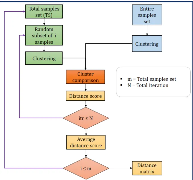
3.1 Workflow diagram of the clustering comparison technique. . . 27

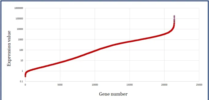
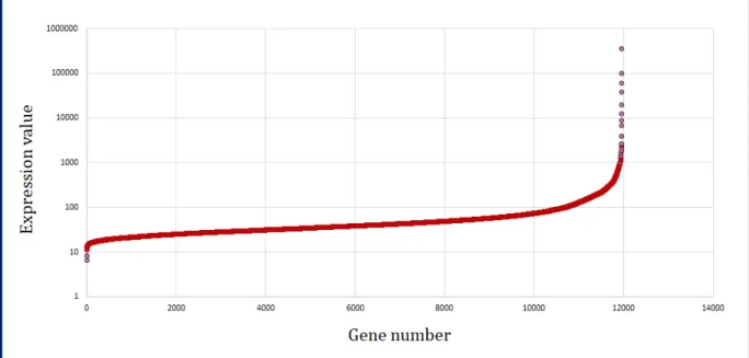
3.2 Sorted mean log distribution of stem cell tissue gene expression data. . . 28

3.3 Sorted mean log distribution ofDrosophila melanogaster multi-tissue, multiple micro-climates data. . . 29

3.4 Sorted mean log distribution ofMus musculus multi-tissue data. . . 29

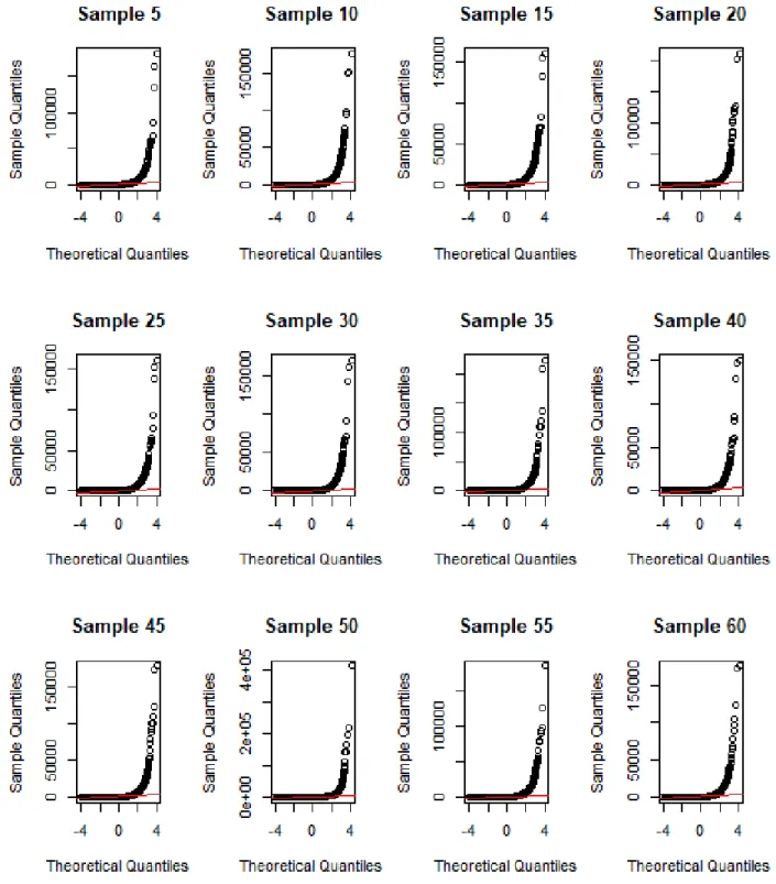
3.5 Q-Q plot of mouse embryonic stem cell tissue gene expression dataset. . . 31

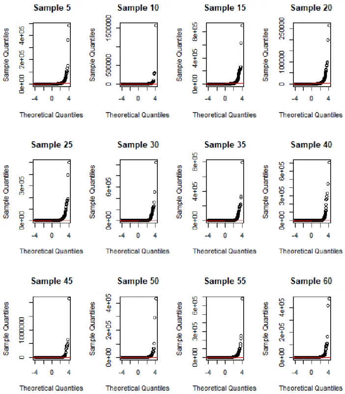
3.6 Q-Q plot ofDrosophila melanogaster gene expression dataset. . . 32

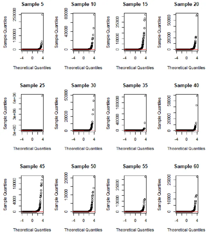
3.7 Q-Q plot of mouse multi-tissue gene expression dataset. . . 33

4.1 Clusterings comparison of mouse stem cell tissue dataset averaged over 100 iterations. . . 36

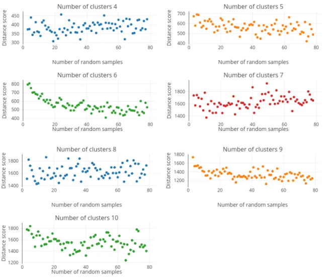
4.2 Comparison of clusterings (K-means V1) with the number of samples verses the average dis-tance score for all numbers of clusters from 4 to 10 of the mouse stem cell dataset. . . 37

4.3 Comparison of clusterings (K-means V2) with the number of samples verses the average dis-tance score for all numbers of clusters from 4 to 10 of the mouse stem cell dataset. . . 43

4.4 Comparison of clusterings (K-means V1) with the number of samples verses the average dis-tance score for all numbers of clusters from 4 to 10 of the mouse multi-tissue dataset. . . 43

4.5 Comparison of clusterings (K-means V2) with the number of samples verses the average dis-tance score for all numbers of clusters from 4 to 10 of the mouse multi-tissue dataset. . . 44

4.6 Clusterings comparison ofDrosophila melanogaster dataset averaged over 100 iterations. . . 49

4.7 Comparison of clusterings (K-means V1) with the number of samples verses the average dis-tance score for all numbers of clusters from 4 to 10 for theDrosophila melanogaster dataset. . . . 50

4.8 Comparison of clusterings (K-means V2) with the number of samples verses the average dis-tance score for all numbers of clusters from 4 to 10 of Drosophila melanogaster dataset. . . . 50

4.9 Spearman’s rank correlation coefficient (calculated from V1 distance score) using various num-bers of clusters for the mouse stem cell tissue dataset. . . 54

4.10 Spearman’s rank correlation coefficient (calculated from V1 distance score) using various num-bers of clusters for the mouse multi-tissue dataset. . . 54

4.11 Spearman’s rank correlation coefficient (calculated from V1 distance score) using various num-bers of clusters for theDrosophila melanogaster dataset. . . 55

4.12 Average clusterings comparing running time for a single iteration using brute force. . . 56

4.13 Average clusterings comparing running time for a single iteration using branch-and-bound. . 56

4.14 Average comparing running time between brute force and branch-and-bound using different numbers of clusters. . . 57

(9)

List of Abbreviations

CCD Cluster Comparison Distance

CD Clustering Distance

CE Classification Error DBI Davies-Bouldin Index

DI Dunn Index

DNA Deoxyribonucleic Acid DSC Dice Similarity Coefficient FMS Fowlkes-Mallows Score

FPKM Fragments Per Kilobase Million GEO Gene Expression Omnibus GFF General Feature Format

GTF Gene Transfer Format

KL Divergence Kullback-Leibler Divergence PCC Pearson Correlation Coefficient

RNA Ribonucleic Acid

RNA-Seq RNA Sequencing

SNP Single Nucleotide Polymorphism

(10)

1 Introduction

Gene expression profiling is a method to identify the activity of genes within cells at a given moment, tissue, or condition [66]. Using the activity of genes, gene expression profiling can help draw conclusions about cell type, state, environment, or biological processes. Gene expression analysis is especially useful for disease diagnosis or drug development. For example, it can help with determining the toxicity of a drug, or the treatment of cancer [79]. It is therefore one of the most important tasks for answering biological questions.

Many modern technologies for expression profiling are high-throughput, and they generate a huge amount of data. Thus, computer analysis has become indispensable to analyze data produced by them. Some com-monly used computer aided techniques for high-throughput expression data analysis are as follows: pattern recognition, data extraction, data preprocessing, data integration, differential expression, clustering analysis, and gene expression time series analysis [38].

Various techniques are used for gene expression profiling. DNA microarrays are a high-throughput hybridization-based technique. A comparatively newer high-throughput technique, RNA-Seq, involves se-quencing RNAs, and it has become widely adopted for studying gene expression profiling. Analyzing RNA-Seq datasets gives several advantages over DNA microarrays; for instance, the ability to detect SNPs (single-nucleotide polymorphisms), and alternative gene spliced transcripts [84].

The first commercially developed sequencing method was Sanger sequencing, developed by Frederick Sanger in 1977. The limitations of Sanger sequencing are mainly due to high sequencing costs and that they require a large amount of time per base to sequence. By way of contrast, modern sequencing platforms are relatively low cost, and are high throughout. Some examples are: Illumina NextSeq500 sequencing (US$42 per gigabase), SOLiD 5500 Wildfire (US$130 per gigabase), Pacific BioSciences RS II (US$1000 per gigabase) [28]. According to the National Human Genome Research Institute (NHGRI), the cost per genome is less than US$1000 (for a genome size of 3000 megabases) — excluding quality assessment, project management, and biological analyses expenses [2]. However, the impact of adding more samples on certain specific data analysis tasks is not well understood, nor are the trade-offs with time and costs.

Differential expression analysis has a pivotal role in gene expression profiling. In an organism, typically, all somatic cells contain the same set of genes. However, the functionality of the genes depends on how they are transcribed and translated in a cell. Genes being expressed differently between cell types was first observed using the DNA-RNA hybridization technique in 1968 [87]. As an example, say there are two patients, where one has tissue cells from an organ that are normal, and the other has a tumor. If there is a

(11)

gene with a large difference in expression levels between the normal and diseased cells, this difference could be important to, e.g. diagnosis or treatment. Hence, analysis of the entire set of RNAs (the transcriptome) is fast becoming a key instrument for differential expression analysis. Generally, differential expression is used to help measure the regulation of genes under differing conditions, or in various groups of samples, or across multiple developmental stages, or for other research purposes [66]. RNA-Seq and DNA microarrays both have emerged as powerful platforms for differential expression analysis.

Another one of the most common data analysis techniques used with expression data is clustering. Clus-tering in general involves grouping together objects into clusters based on similarity or dissimilarity. That is, the primary goal of clustering is to divide objects into sets, called clusters, such that objects within clusters are highly similar to each other, and more diverse relationships exist between objects in separate clusters. Grouping objects (in our case, genes) also plays an important role in gene expression analysis. Typically, genes are defined to be similar if they have similar expression patterns. When genes are grouped together based on this type of similarity, this can provide evidence of related functionality, or that they are involved in some joint process. Cluster analysis can also be applied to find out different gene expression patterns on a small subset of genes [79].

Cluster analysis is a process of data exploration. Data is commonly presented in two formats: a data matrix and a distance matrix [91]. In the data matrix, genes are represented as rows, and samples are represented as columns, with entries being expression values. The distance matrix is used to show the similarity or the pairwise distances between two or multiple gene’s expression values. Distances are created based on the data matrix, and a distance function (calculating the distance between two objects); for example, Euclidean distance. A higher distance between two genes expression patterns indicates lower similarity among them. Then, clustering can be performed from the distances in the distance matrix. Clusterings depend highly on the clustering algorithm used. Even the same datasets can give different results depending on which algorithms are being used.

The term clustering comparison refers to the process by which clusterings are analyzed and compared. A comparison can be used for two things: in particular, if a “correct answer” is known, then one could assess closeness between the true clustering and the predicted clustering. Additionally, comparisons might help to assess consistency of clusterings. Here consistency refers to how clusterings vary depending on the sets of samples used to construct them. Indeed, although cluster analysis is often used when no known ground truth information is known, with sufficient data, it is possible to assess the consistency of clusterings. This can be thought of as validating the clusterings in terms of approaching some local maxima. When clusterings are compared, some distance function is required (not to be confused with the distance function to create the clusterings). In this context, a small distance indicates similarity and large distance indicates dissimilarity between two clusterings.

The main objectives of this thesis are to:

(12)

clusterings — primarily focused on RNA-Seq datasets. This proposed distance should be easy to apply and interpret in the context of gene expression clustering.

2. Investigate different algorithms for computing the cluster comparison distance exactly.

3. Test the effect of adding more biological samples to existing RNA-Seq expression datasets on K-means clusterings, in order to find a relationship between the number of biological samples and clusterings.

The third objective can be done with the help of the work on cluster comparison and the algorithms from the first and second objectives. This could help in understanding the trade-offs between the number of samples and the clusterings, which could help to reduce the number of samples needed for certain types of analysis. This analysis could provide an effective method to either reduce costs by requiring fewer samples in certain situations, or an understanding of the benefits additional samples would bring. Although the small number of datasets tested (three) limits the ability to make general conclusions, the results, plus the general approach provide an important contribution to research on gene expression profiling using RNA-Seq gene expression data by creating a methodology to assess how clusterings change as the number of samples increase.

This thesis is composed of five chapters. Chapter 2 contains the background, and begins by laying out the theoretical aspects of the research; it introduces the basic gene expression profiling techniques and provides a brief description of supervised (e.g. classification and regression analysis), and unsupervised (e.g. clustering) learning. Distance functions for clustering are also described in this chapter, which are one of the important parameters for a clustering algorithm. A study of existing clustering comparison methods is also presented. Chapter 3 describes the methodology, tools, and techniques that are used for this research. It describes the data normalization pipelines used for the RNA-Seq datasets analyzed. The three datasets used to test the methodology (mouse embryonic stem cell tissue, Drosophila melanogaster from multiple tissues and micro-climates, and mouse data from multiple tissues) are also described. This chapter also provides a detailed explanation of the different implementations of the comparison method, and the method used to assess consistency of clusterings with additional samples. Chapter 4 presents the results of the consistency of clusterings on all three datasets. A statistical analysis, an analysis of performance, and an assessment of the effectiveness of the clustering comparison results are presented in this chapter as well. The latter part of Chapter 4 discusses some implications of the results. Lastly, Chapter 5 gives a general review of this research work, describes the limitations of the proposed methods, and gives an overview of future directions.

(13)

2 Background

DNA is a macromolecule that encodes information in the form of chromosomes. Chromosomes copy infor-mation via DNA replication [35]. The central dogma of molecular biology states that the flow of inforinfor-mation between molecules is mainly from DNA to RNA, and then RNA to protein (see Figure 2.1) [66, 35]. From a protein molecule, information will never pass back to nucleic acid. The central dogma can be divided into two parts. One is the transfer of information, and another is the conversion of information into other forms.

Figure 2.1: Central dogma of molecular biology.

Transcription is the process of creating RNA from DNA. Here, an enzyme called RNA polymerase reads the DNA, and produces an RNA molecule [35]. Then, in some genes of eukaryotic organisms, certain sections of RNAs, called introns, are removed, leaving the remaining sections, called exons. For protein coding RNAs, this produces messenger RNA (mRNA). In the process of translation, mRNA is converted into proteins, which is another type of macromolecule that consists of a chain of amino acids. The structure or the three-dimensional shape of a protein largely depends on the sequence of amino acids present in the polypeptide chain, and the structure largely dictates its function [94].

Both coding and noncoding RNAs (those that do not get translated to protein; e.g. tRNA, rRNA, etc.) together are called the transcriptome. Gene expression profiling is used to quantify the amount that each RNA sequence occurs in a set of cells from some tissue of an individual at a given time. This is usually multiple cells unless using single cell RNA-Seq. However, the amount of each RNA present varies from cell to cell, and tissue to tissue.

(14)

2.1 Gene expression profiling techniques

Different techniques are used for gene expression profiling. Early methods were low throughput and expensive [84]. More recently, high-throughput methods have become more common, which will be the focus of this work.

2.1.1 DNA microarrays

Variation in gene expression can be analyzed using microarrays. A DNA microarray or DNA-chip, is a glass slide that can contain thousands of microscopic DNA probes on its surface. DNA microarray technology uses the following two general steps [67, 84]: first, the production of a DNA microarray for a particular organism, and second, gene expression profiling of that organism’s experimental cells to measure the transcriptome. DNA microarrays, often produced by chemical synthesis, can involve attaching short 20−30 base pairs of single-stranded DNA, called probes, to the glass slides. Frequently, probes are constructed for each gene in an organism.

Two types of cells are commonly used for DNA microarray analyses. These are the control and targeted cells. Normal (or healthy) cells, and mutated (or diseased, or treated with a drug, etc.) cells of a particular organism are treated as control and target cells, respectively [67]. First, mRNA is extracted, then reverse transcribed into complementary DNA. Colour dyes (cyanide dyes) are applied to allow fluorescent intensity to be measurable. Then, these cells are placed onto the DNA microarrays (often separately). Hybridization occurs when one single-stranded copy of DNA binds to another complementary single-stranded DNA of one of the probes [26, 61]. After hybridization, a computer scanner is used to measure the amount of fluorescence label. Therefore, by looking at the intensity of the fluorescent labels, the quantity of each RNA sequence can be estimated. An alternative approach to using two types of cells are time trials, where samples are collected at multiple times of some biological process.

2.1.2 RNA-Seq

RNA-Seq, also called whole transcriptome shotgun sequencing (WTSS) [29, 84], involves sequencing RNAs in a sample using next-generation sequencing. This can determine which genes are active, and also estimate the amount of each mRNA produced at a certain time.

The first phase of RNA-Seq experiments is library preparation [84]. This involves RNA isolation, possible filtering, and then cDNA synthesis from the RNAs [28]. Sequencing the library is the second phase, which produces fragments of the cDNAs called reads. If an assembled genome already exists for the organism, the RNA-Seq reads can be aligned to the genome in a process called read mapping. Or if an assembled genome does not exist, the transcripts can be assembled into full RNAs in a de novo fashion. Then all transcript sequences are counted. Without normalization, it is not possible to compare expression levels between and within samples accurately. Li et al. [50] proposed a guideline for the selection of the most

(15)

appropriate normalization methods for experiments. Various normalization methods can be used, such as the non-abundance method, the abundance method, or the inter-sample method [50].

After read mapping and normalization of all reads sequenced, the data matrix is generated (see Figure 2.2). Each row represents a single transcript, and each column represents an individual sample.

Figure 2.2: The yellow coloured box indicates gene names, the green colour box represents the sample numbers, and orange colour box shows the count for that gene in each individual sample.

Data analysis is the final phase (for both RNA-Seq and DNA microarrays) of gene expression analysis. Firstly, it is common to assess differential expression, which involves calculating which genes are significantly different between the control and target sample sets. Clustering techniques are also widely applied in gene expression analysis. Cluster analysis can expose unknown connections among genes based on similar or correlated expression. Using gene expression profiling, clustering can also be helpful for pathway analyses of co-regulated genes [66]. Clustering will be discussed further in Section 2.2.2.

2.2 Machine learning

Machine learning and classification are important problems in engineering and scientific disciplines, and have been frequently applied to problems in biology, medicine, marketing, and many others. Classification involves the assigning of a discrete label to unlabelled data. Watanabe [86] defines a pattern “as opposite of a chaos; it is an entity, vaguely defined, that could be given a name.” A pattern could be a DNA fragment, an image of a handwritten cursive word, or it could be a speech signal. The recognition or classification can be categorized into two types: supervised classification and unsupervised classification. The aim of predictive or supervised learning is to map from input patterns to output patterns, given a (separate) set of a priori known input-output pairs called the training set. Input patterns consist of features, attributes, or covariates, in general. It could be of complex structure, a molecular shape, a graph, etc. [37]. The second main learning

(16)

approach is descriptive or unsupervised classification, sometimes called knowledge discovery. Figure 2.3 shows a characterization overview of machine learning algorithms.

For both supervised learning and unsupervised learning approaches, parameters need to be set to develop a probabilistic model [60]. If a fixed number of parameters are used in the model, then it is called a parametric model. Supervised classification algorithms use parametric models. When the number of parameters increases depending on the sample size, then it is called a non-parametric model. Parametric models tend to be faster than non-parametric models [60]. However, for large datasets, strong prediction is often easier by using a non-parametric model, as it gives high flexibility to fit the data. However, it can often cause an overfitting problem, whereby a model is dominated by random samples or noise instead of by general patterns. Overfitted models are excessively complex; with such a model, a learned hypothesis may fit the training set very well, however it fails to generalize to new examples.

Cross-validation is an evaluation technique for validating a predicted model [60]. Learning approaches, like supervised learning, can use cross-validation for analyzing the outcome of a prediction. It can also be used to test how well a model can perform when real samples are applied. K-fold cross-validation divides the training sample into K equal sized parts. After that, it considers the first part for testing while using the remaining parts for training. Then, the second part is used for testing, etc., and the process continues for each part. Before applying testing samples, it is helpful to use cross-validation to check the performance of the model. It also helps to understand how results of the statistical analysis will generalize to the entire dataset.

2.2.1 Supervised learning

Two common supervised learning approaches are classification and regression, which will be briefly described. Classification is a process to identify or categorize the features of a set of problems based on predefined labelled datasets. Classification varies depending on the features. If there are two different types of features, then it is called binary classification. If the features are classified into more than two types, then it is called multiclass classification. Multi-label classification can be mutually exclusive or not [60]. Features or attributes are often called explanatory variables. These features can be categorized in various ways; for instance, categorical (boy or girl), real-valued (temperature), integer-valued (frequency of arrival at a particular place), nominal (price range), or ordinal (rank of position).

A classifier is simply a mathematical function that is used to “solve” (by assigning labels to each item) a particular supervised classification problem. The goal of a classifier is to predict the outcome with maximum (or close to maximum) accuracy based on the labelled dataset. It can be formalized as calculating a function,

y =f(x), where y is the outcome, and xis in the predefined dataset. In machine learning, outcomes are often referred to by classes, and the predefined dataset types are called features or a feature vector [7].

Classifier performance evaluation is sometimes described as having “no-free-lunch”, meaning that no single method is suitable for all kinds of classification problems [89]. A classifier performance depends on the

(17)

characteristics of the training set, and choosing the right classifier should be found according to the problem specified.

One common example of a classification problem is detecting whether an email is spam or not. In this case, the training set can be built with regular email (i.e. non-spam) and spam email. Here, large data samples help the classifier to distinguish an email into a correct class. Other classic classification applications are in the areas of computer vision, drug discovery and development, handwriting recognition, speech recognition, biological classification, etc.

A problem is called a regression problem when the features are nominal (scalar real-valued) variables. Statistical regression is the prediction of the relationship among the dependent variable with one or multiple independent variables [60]. Various techniques are applied to predict the impact of independent variables on the dependent variable. For example, the input features or the experimental setting or the environmental factors on a given problem can be set as the independent variables. A dependent variable is simply the outcome of the experimental result or the solution of a particular problem. Specifically, regression analysis helps to predict or assume the influence of a single independent variable to the dependent variable.

Regression analysis performance widely depends on the data generating process and the choice of method used. A regression model z can be defined as: z≈f(x, c), and approximation can be formalized as: E(z |

x) =f(x, c), where xis the independent variable(s), and the unknown factor isc. The functionf must be defined between dependent and independent variables based on prior knowledge [60].

Linear regression: Linear regression creates a relationship between a dependent variable and indepen-dent variables. A regression line is used to build this relationship, which is a best fit straight line. An example is y=a+bx+cn, wherecn is an error term for eachn(number of data points); aand b are the intercept

and slope, respectively. Simple linear regression occurs when the number of independent variables is one. Multiple independent variables are used for multiple linear regression [60].

Some other popular regression analyses are: polynomial regression and logistic regression. Polynomial regression is similar to linear regression except for the exponent on the independent variables. Higher order polynomial regression often has a lower error rate [60]. Depending on the independent variables or input features, logistic regression develops a model of probability for an event occurring. Logistic regression gives the estimation of a probability based on an event occurring or not occurring.

2.2.2 Unsupervised learning

Unsupervised learning is a predictive model, where datasets are not previously labelled, and also there is no defined output format. The outcome of this learning approach always depends on the observations. Unsu-pervised learning methodology looks for common patterns or structures in the testing data samples. It is a sort of a similar learning technique to how a human or an animal learns. It gains knowledge through expe-riences and from the environment. Unsupervised learning systems infer output without any prior knowledge or predefined labelled data.

(18)

Unsupervised learning methods develop a density estimation (constructs a probability distribution model based on unlabelled random responses) model for each input rather than defined outlines, like supervised learning [60]. Comparing the supervised learning technique to unsupervised learning, there are primarily two differences [32]. Because supervised learning predicts a single outcome for particular input variables, then it uses univariate probability density estimation. On the other hand, an unsupervised learning outcome is a vector of features; therefore, multivariate probability models are needed.

One of the most important types of unsupervised learning methods is clustering. The primary goal of clustering is to group data elements based on similarity or dissimilarity. It creates smaller subsets or partitions of related data. In various disciplines, clustering techniques are widely applied. For example, based on internet browsing history or interest, customers are being clustered by e-commerce sites to increase sales, and also to help to find target consumer groups. In biology, gene expression analysis uses clustering techniques to group sequences based on similar expression patterns. Clustering can be used as a stand-alone tool and also, can be used as a processing tool for other algorithms.

Clustering finds structure in a collection of unlabelled instances. For example, consider a collection ofn

objects, xi, 1≤i≤n; eachxi is ap-dimensional feature vector. Then, one goal with clustering is to divide

thesenobjects intok(a fixed number) of clusters such that the objects within a cluster are more “similar” to each other than objects between clusters. But what does this mean? There is no single answer — it depends on what distance is used to assess similarity on the data. For this reason, clustering is often referred to as an “art.”

Two different types of clustering algorithms exist: strict partition clustering (each object is placed in some cluster and is not placed in more than one cluster) and overlapping clustering (cluster results may overlap) [93]. An example of strict partition clustering is K-means clustering, and an example of overlapping clustering is the expectation maximization (EM) algorithm. Some other popular clustering methods are hierarchical, self-organizing maps (SOMs), and mixture models.

Clustering is useful for identification of genes (in our case, these objects are genes) that are “working together” or that are co-related. This is beneficial for biological identification of distinct functional subgroups. A good clustering method will produce clusters with high intra-class similarity (objects that are similar belong to a single cluster) and low inter-class similarity (higher the distance for objects in different clusters) [93]. Seen as a graph where objects are connected if their distance is small, then after clustering, objects in the same cluster are connected densely, and only sparse connections exist between different clusters.

One unsupervised clustering method of interest is K-Means clustering. The goal of the K-means clus-tering problem is to partition a set of objects into K subsets or K clusters in order to minimize the within cluster variance [41]. The problem is NP-hard in general [6], and therefore any exact algorithms to solve it likely requires more than polynomial time complexity, and therefore heuristic algorithms are needed. A heuristic algorithm often called the K-means algorithm is commonly used for K-means clustering [52]. The approach of the K-means algorithm starts from an initial partition of the objects (e.g. genes) and proceeds

(19)

by iteratively calculating the centers (means) of the clusters and then it reassigns each object to the closest cluster according to some measurement of distance such as Euclidean distance. This iteration continues until no more reassignments take place. From a computational perspective, this heuristic K-means algorithm is relatively efficient as it has a time complexity ofO(tkn), where nis the number of objects,kis the number of clusters, and tis the number of iterations, which is why the heuristic algorithm is more commonly used than the exact algorithm. Notice that this heuristic K-means algorithm is not deterministic in the sense that running it multiple times on the same input will often give different results.

Figure 2.3: An overview of machine learning algorithms [60].

Distance functions

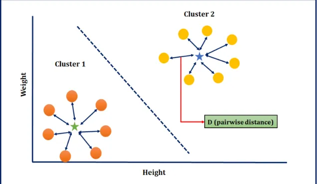
The objective of cluster analysis is to group objects based on similarity. Distance functions used for the purposes of creating clusterings will be called clustering distances (CD). These kinds of distance functions quantify the distance between two sets of objects, which can be used to measure similarity. Given a distance function, the goal with clustering is to place elements into clusters in order to minimize the intra-cluster distance, and maximize the inter-cluster distance (see Figure 2.4) [93]. Deza et al. [22] published a book named “Encyclopedia of Distances” which is one of the leading references of distance metrics, and covers most of the active research areas in distance functions.

(20)

Figure 2.4: Each circle is a different person’s height (x-axis) and weight (y-axis). There are two clusters represented by orange and gold colour balls respectively. Green and blue colour stars (cluster center) indicate the pairwise distances within each cluster.

Euclidean Distance, Minkowski Distance, Pearson’s Distance, Hamming Distance, and Manhattan Distance, which are described next.

Euclidean distance

Euclidean distance is a simple distance measurement that can be used in Euclidean space. It measures the dis-tance between points inn-dimensional space. In Cartesian coordinates, for two vectorsa= (a1, a2, a3, . . . , an),

b= (b1, b2, b3, . . . , bn), the Euclidean distance betweenato b(orb toa), is defined as follows:

DE(a, b) = r (a1−b1) 2 + (a2−b2)2+· · ·+ (an−bn)2 .

For example, say a and b are both vectors with five components, a = (5,6,9,10,18) and b = (3,8,9,8,20). Then the distance DE(a, b) =

r

(5−3)2+ (6−8)2_{+ (9}₋₉₎2_{+ (10}₋₈₎2_{+ (18}₋₂₀₎2_.

Therefore,DE(a, b) = 4.

Another variant of Euclidean distance is Euclidean squared distance,

D2_E(a, b) =(a1−b1)2+ (a2−b2)2+· · ·+ (an−bn)2

.

Euclidean squared distance and Euclidean distance both use almost the same base equation. Although, Euclidean distance is suitable for small distance calculations, using the Euclidean squared distance in clus-tering algorithms is faster in comparison to using Euclidean distance [60].

(21)

The Euclidean distance from the origin to a vector is a called the Euclidean norm or Euclidean magni-tude [16]. That is, the Euclidean norm ofa= (a1, a2, . . . , an) is:||a||=

p

a2

1+a22+· · ·+a2n.

Manhattan (city-block) distance

The Manhattan distance or city block distance is defined as the sum of the absolute differences of each component of the two points in Cartesian coordinates [14]. Here, the distance is equal to the length of all shortest paths connecting to aandb along horizontal and vertical segments. For n-dimensions data points,

a= (a1, a2, a3, . . . , an) andb= (b1, b2, b3, . . . , bn), then the Manhattan distance is:

DM n(a, b) = (|a1−b1|+|a2−b2|+· · ·+|an−bn|).

For example, given two pointsa= (2,2) andb= (3,1), the Manhattan distance betweenaandbisDM n(a, b) =

(|2−3|+|2−1|) = 2

The name Manhattan distance came from the grid layout of most streets in Manhattan Island [14]. Often Manhattan distance is called the L1 distance (norm), which is the summation of the absolute values of

two sides in a right angled triangle. Manhattan distance is employed for discrete frequency distribution. For example, to compare the positional distribution of hexamers in RNA splicing, Manhattan distance is used [51]. It is also used in sparse sampling (also known as compressed sensing) which is a signal processing technique in an undetermined linear system for acquiring and reconstructing a signal.

Minkowski distance

Minkowski distance is a generalized form of both Euclidean distance and Manhattan distance [14]. It is a distance function which can be defined as the norm (length of the vector) in a norm vector space. The general form of Minkowski distance is calledLmdistance. The Minkowski distance of ordermbetween twon-tuples

points is given below: fora= (a1, a2, a3, . . . , an) andb= (b1, b2, b3, . . . , bn),

DM i(a, b) = (|a1−b1|m+|a2−b2|m+· · ·+|an−bn|m)

1/m

.

Another variation of Minkowski distance is weighted Minkowski distance,

DM i(a, b, w) = (w1|a1−b1|m+w2|a2−b2|m+· · ·+wn|an−bn|m)

1/m

,

where weights w= (w1, w2, w3, . . . , wn) are chosen based on the application.

Pearson’s distance

Based on Pearson’s correlation coefficient, Pearson’s distance is calculated between twon-tuples to measure their linear relationship [22]. For a = (a1, a2, a3, . . . , an) and b = (b1, b2, b3, . . . , bn), then the Pearson’s

distance is:

(22)

wherer(a, b) = Pn i=1(ai−a)(bi−b) pPn i=1(ai−a) 2pPn i=1(bi−b)

2, withathe mean of values ina, and similarly withb, is Pearson’s

correlation coefficient between aandb.

Canberra distance

Canberra distance is a weighted form of Manhattan distance developed and improved by Williams Lance and Adkins in 1966 [44]. It measures distances between scatter data or to group individuals from an origin. For

n-dimensions data points,a= (a1, a2, a3, . . . , an) andb= (b1, b2, b3, . . . , bn), then the Canberra distance is:

DCa(a, b) =

|a1−b1|+|a2−b2|+· · ·+|an−bn|

|a1+b1|+|a2+b2|+· · ·+|an+bn|

.

χ2 distance

To calculate the distance between two histograms, a distance metric called χ2 distance can be used [39]. In theχ2 _{distance, two histograms (discrete probability distributions) should have an equal number of bins to}

calculate the difference between them. It is often used for document classification in computer vision (which is called the bag-of-words model). Aχ2_{distance is a weighted form of Euclidean distance. Given an observed}

value a = (a1, a2, a3, . . . , an), and an expected value b = (b1, b2, b3, . . . , bn) having n bins, theχ2 distance

betweenaandbis as follows:

Dχ2(a, b) = 1 2 X (ai−bi) 2 /(ai+bi) . Hamming distance

The Hamming distance function is used to calculate the distance between two categorical variables [31]. Here, 0 indicates a similar feature of two categorical variables, and 1 otherwise. The Hamming distance is obtained after adding all those differences. For example, ifaandbare two categorical variables ofdfeatures, then the Hamming distance between aandbis as follows:

DH(a, b) = d

X

i=1

(ai⇔bi),

where (ai⇔bi) = 0 if and only ifai andbi indicate similar features, and 1 otherwise.

Kullback–Leibler divergence

In machine learning, Kullback–Leibler (KL) divergence is used to measure the distance between two distribu-tions [43]. It measures the divergence of a probability distribution from a reference probability distribution. The KL divergence score varies from 0 to 1. Here, 0 indicates that the two distributions are the same or there is no difference between them, and 1 depicts that comparing distribution shows a different pattern than the reference distribution. IfP andQare two probability distributions, then the KL divergence betweenP and

(23)

Qis: DKL(P||Q) = Z x∈D p(x) logp(x) q(x)dx,

where,p(x) andq(x) are the probability density ofP andQrespectively, andxis in the range of domainD.

2.3 Cluster comparison

A cluster comparison is a measure of similarity between two different clusterings. The two clusterings could have been produced by the same algorithm using different parameters, by using different algorithms altogether, or using the same algorithm by using different subsets of the data. It could ultimately be used as a technique to validate clusterings.

It is necessary to clarify exactly what is meant by clustering comparison. As previously mentioned, a group of similar instances that have been grouped together is called a cluster. When multiple clusters are created from a dataset, this is a clustering. The comparison between two clusterings is called a clustering comparison. Just as distances are used to create a clustering, distances can also be used to compare two clusterings. The distance functions used to compare two clusterings are called cluster comparison distances (CCD). It is important to keep in mind the differences between CDs (clustering distances) and CCDs. In this context, a lower distance score indicates that two clusterings are similar. This score can be used as an indication of a clustering algorithm’s quality if a correct answer is known.

Meil˘a [56] surveyed different cluster comparison methods. Here, only cluster comparisons of strict partition clusterings will be discussed. LetX be a set ofnelements: X ={x1, x2, x3, . . . , xn}. Next, letG1andG2be

two clusterings, whereG1={P1, P2, P3, . . . , Pk}andG2={Q1, Q2, Q3, . . . , Ql}. Each element ofG1andG2

is a subset of X, and the elements ofG1 orG2 are disjoint sets, such thatSk_i₌₁Pi=X, andSl_i₌₁Qi =X.

Thus, G1 and G2 are sets of disjoint sets of elements of X whose union is the set of all elements. For

example, if X = {x1, x2, x3, x4}, and k = l = 2, then one possible clustering could be: G1 = {P1, P2},

where P1 = {x1, x2, x3} and P2 = {x4}, and another possible clustering could be G2 = {Q1, Q2}, where

Q1 = {x1, x3} and Q2 ={x2, x4}. A clustering comparison distance measures the difference between the

elements inG1andG2.

A similar task is cluster evaluation which can be used to assess the quality of clusterings. Evaluating or validating clusterings is a difficult task. As clustering is often used as an unsupervised method (if the ground truth is unknown), it is hard to evaluate a clustering [60]. Popular approaches of evaluating clusterings fall into two groups: internal evaluation and external evaluation. An internal evaluation technique is only evaluated within a clustering (e.g., Dann index). External evaluation can be applied when a predefined or reference clustering is available (e.g., purity).

There are several techniques used for clustering evaluation and cluster comparison, which are discussed in the next section.

(24)

Cluster comparison distances

One natural approach for comparing clustering is pair counting. This classifies each pair of objects in discrete categories and then counts the results. A pair of unordered objects can be classified in four different ways: 1.

the pair appears in the same cluster of both clusterings, 2.the pair does not appear in the same cluster within both clusterings, 3.the pair appears in the same cluster of the first clustering, and in different clusters of the second clustering, or, 4.the pair appears in the same cluster of the second clustering, and different clusters of the first clustering. Several mathematical measures are found in the literature for cluster comparison based on the pair counting technique, such as Rand index [68], andχ2 _{coefficient [64].}

The Rand index is the ratio of the number of elements where both clusterings put them in the same cluster, plus the number that are placed in different clusters of both clustering, divided by the total number of pairs. The range of Rand index varies from 0 (all pairs that appear in the same cluster of one clustering appear in different clusters of the other clustering, and vice-versa) to 1 (each pair either appears in the same cluster of both clusterings, or in different clusters of both clusterings). If it is preferred, one minus the Rand index gives smaller values for similar clusterings. Different variations of Rand index exist in statistics; for example, adjusted Rand index is commonly used [75]. Albatineh et al. [5] give a list of 28 comparison measures based on Rand index and pair counting. However, some of the measures become equivalent after making some changes to the pair counting technique [85].

Meil˘a [56] presents a Classification Error (CE) metric between two clusterings. Let G1 and G2 be two

clusterings where G1 has K clusters, G2 has K0 clusters and K ≤ K0, and n be the number of elements

clustered. Then DCE(G1, G2) = 1−_n1maxσPK_k₌₁nk,σ(k), where σ is any injective mapping function to

match clusters of G1 to G2 (injective means no two clusters of G1 map to the same cluster of G2). The

author mentioned that despite the at leastK! possible injective mappings, the maximal bipartite matching algorithm in graph theory can calculate the distance exactly in polynomial time. Meil˘a also points out that CE distance is simple and intuitive, especially when clusterings are similar.

Probabilistic approaches use likelihood to compare clusterings. One commonly applied technique is to compute the distance between two probability distributions. One method for this is called EMD (earth mover’s distance) [48, 72]. Here each clustering represents a distribution. To compare the distributions, it first fragments each of them. The EMD can then be calculated by measuring the distances between each fragment of the two distributions. To get the final EMD between two distributions, it adds all the distances between each fragment.

Mutual information of two clusterings measures the number of common objects obtained from one clus-tering compared to the other. The mutual information is inspired by the idea of entropy theory (calculating the missing information) [20]. One of the variations of mutual information is adjusted mutual information (AMI) [81]. The adjusted mutual information measure is often used to calculate the similarity between two clusterings. It measures two clusterings based on their distribution of results. If two distributions are randomly distributed, then AMI returns 0; otherwise, it returns 1 which means the two distributions are

(25)

identical.

Another common technique, named word mover’s distance (primarily focused on text matching), measures the relatedness of two words by measuring the closeness in meaning [83]. One of the pioneer researchers of distribution-based clustering comparison is Marina Meil˘a [56, 33, 55, 57]. Meil˘a introduced more partitioning properties in cluster comparison using entropy theory. D. Zhou et al. [93] proposed a clustering comparison metric for global optimization, inspired by the Mallows distance — computing the distance between two distributions. For clustering comparison, the authors use both strict partition clustering and overlapping clusterings.

Clustering evaluation metrics

Validity measure, or v-measure, is an external measure of clustering, and it uses a ground truth clustering. For a given clustering, completeness and homogeneity metrics are calculated. A clustering satisfies the completeness if all class members (data points) are in the same cluster compared to the reference class. A clustering satisfies homogeneity when each of the class members are in the same class label and in the same cluster compared to the reference clustering. Rosenberg et al. [70] combined these into v-measure to evaluate a clustering. Its scores are calculated by using the harmonic mean of homogeneity and competence values.

Purity is another external measure of clustering quality for overlapping clusterings [60]. It measures the intra-cluster similarity. Purity only considers majority clusters and numbers of objects of those majority clusters. Then, it counts the maximum number of objects in each cluster, and adds those maximum counts. Therefore: purity = 1

N

P

i∈kmaxj(nij), where, kis the set of clusters, N is the total numbers of objects,

andnij indicates the numbers of objectsj in a clusteri. Its scores vary from 0 (poor similarity) to 1 (good

similarity). However, purity never penalizes different cluster sizes in clusterings, and a major drawback of purity is its often high value.

Set matching or set overlaps are primarily used for document classification. Set matching defines a set of objects which are common to both clusters. A classic example of a scoring metric for set matching is F-score (defined below). There are other measurement tools that are available based on set matching, for example, Van Dongen-Measure [23, 82]. For error counting or to test the accuracy, F-score is commonly used in set matching [47]. F-score is used as a binary classification — positive or negative — and is also called the harmonic mean of precision and recall. Here, precision is the ratio of the numbers of correctly identified results divided by all positive results returned by a classifier. The recall is the ratio of the numbers of correctly identified results divided by the number of true positives plus false negatives. Then,F–score=

2(precision×recall)

precision+recall . The F-score varies from 0 (total incorrect prediction) to 1 (correct prediction). Based on

the principle of precision and recall, another clustering comparison metric — Fowlkes-Mallows score — is generally used. The Fowlkes-Mallows score depends on the predefined clusterings, which is used as a reference or a benchmark [27]. Fowlkes-Mallows scores can be defined as a geometric mean of precision and recall:

(26)

TheR2 _{coefficients is defined by the summation of within cluster and between cluster sum of squares,}

which can be used as an evaluation metric for unsupervised clusterings [74].

Silhouette coefficient is another clustering evaluation metric [71]. It is a graphical tool which is used to test the validity and consistency of clusterings. Such a comparison depends on the variance of clustering elements. A lower variance between cluster elements and higher variance within clusters is expected for better similarity. Predefined labelled or reference output is not necessary for silhouette index score. However, the computational cost is high for higher cluster size. Its scores vary from−1 to +1, where−1 indicates incorrect clustering, 0 and +1 represents overlapping and dense clustering, respectively.

David et al. [21] introduced an internal clustering comparison metric named the Davies–Bouldin index (DBI). The DBI index primarily focuses on the assignment of objects within a cluster. It measures the distance of each object in a cluster from the centroid of the cluster. By comparing the distance within a cluster, the DBI validates clusterings — how well clusters are created. The norm distance function is generally used to calculate the distance from a cluster centroid to each data object.

Dunn [25] proposed another clustering evaluation metric which is referred to as the Dunn index (DI). The Dunn index calculates the mean difference of within-cluster objects compared to between cluster objects. A high score of DI indicates that objects within a cluster are densely connected, and sparse connections exist between different clusters. One of the limitations of DI is high execution time as the cluster size and numbers of data points increase.

Based on the dispersion of cluster objects, the Calinski Harabasz (CH) measure was developed for compar-ing clustercompar-ings [17]. The CH metric is calculated by the ratio of within and between cluster dispersion scores (variance of a distribution). A higher CH index shows that objects within a cluster are densely connected and are well separated by the other cluster objects.

Other frequently applied clustering evaluation metrics are the following unsupervised evaluation tech-niques: Gamma and Tau [13], C-Index [34], Gap statistics [76], I-Index [54], S Dbw (separation and density based) [30], DBVC (density based cluster validation) [59], and the following supervised evaluation techniques: B-Cubed evaluation [12], Set matching purity [92], Gini-based evaluation [73].

Other related works

To characterize a clustering, and to overcome the limitation of previously existing clustering comparison techniques, E. Bae et al. [11] proposed a density profile to measure the similarity. The proposed comparison method is ADCO (Attribute Distribution Clustering Orthogonality), which is inspired by the area of data mining. Here, the similarity between two clusterings depends on the prediction model, and two clusterings are more likely similar if the two predictive models are similar. Additionally, other methods are proposed, for example, to identify structural dissimilarity, and to compare non-overlapping clustering methods.

To minimize the error rate of different clusterings, Backer and Jain [10] suggest various partitioning techniques for different clustering algorithms. For clustering validation, S. Monti et al. [58] used unsupervised

(27)

learning algorithms (K-means, SOM, etc.) on DNA microarrays of gene expression datasets. They show that the experimental results (both simulated and real data) are biologically meaningful for cluster analysis.

2.4 Tools for machine learning and for clusterings comparison

Due to the diversity and complex nature of bioinformatics problems, it is important to choose the right tool for the given task [24]. In our case, the tool often dictates a programming language. The most popular modern interpreted scripting languages are Perl, Python, and R. There are many reasons for using these languages: for example, memory management, code readability, dynamic type system, and the ability to build prototype programs in an interpreted and extensible environment [24].

For scientific computing, a number of open-source frameworks are commonly used. For example, NumPy, SciPy for Python, Ruby on Rails, etc. Besides that, many other structured frameworks particularly designed for bioinformatics are available, such as BioPython (Python), BioJava (Java), BioConductor (R), BioPERL (Perl), and BioRuby (Ruby). These structured frameworks are well documented, rigorously scrutinized, and involve an enthusiastic community providing regular improvement.

A scripting language is also often used for automating the execution of tasks using the run-time environ-ment. They can combine complex programs or API calls, and can be used as a domain specific language.

The main difference between a compiled language and a scripting language is its compilation step. To run a program, compiled languages require a compiler to convert into some other format of code, either machine code or some higher-level intermediate code such as Java’s bytecode. On the other hand, scripting languages can execute a program without compiling the entire program in advance. Scripting languages can make it easier for the developer to modify functionality. In the case of Python, it can work both as a compiled language (use CPython for implementation, convert source code into bytecode, then return the bytecode in a virtual machine), and a scripting language as well.

Here two main platforms are used: VLFeat (MATLAB) and Python scikit-learn. R is also used for some statistical analysis.

VLFeat

VLFeat is an open source MATLAB library [80]. It is a collection of cross-platform classes and packages, primarily developed for popular computer vision algorithms, with a special focus on local feature extraction, and the matching of images on large datasets. Of interest, VLFeat has implemented a large pool of machine learning algorithms. For example, the following statistical methods are included: GMM (Gaussian mixture model) using the expectation maximization algorithm, K-means, SVM (Support vector machine), KD-trees, etc. There are many visual features implemented, for instance, covariant detectors, HOG (histogram of oriented gradients), SIFT (scale invariant feature transform), dense SIFT, Fisher vector, and many others. VLFeat provides a C wrapper function for other programming languages and supported on multiple platforms,

(28)

for example, Windows, macOS, and Linux. The MATLAB interface is an easy way to use the VLFeat library that allows to run the same algorithm on different platforms.

Python scikit-learn

Scikit-learn [65] is a toolkit of SciPy (Scientific Python). It is primarily developed for machine learning algorithms. Data distribution, filtering, aggregation, and classic machine learning algorithms are implemented in the scikit-learn library. For instance, classification clustering algorithms — K-means, K-nearest neighbor (KNN), hierarchical clustering; regression algorithms, support vector machine (SVM), etc. Standardized tools are available for data preprocessing, and it is easy to create one’s own model to fit the test data using scikit-learn. Multiple library functions are available for evaluating model’s performance; for example, classification matrices (accuracy score, classification report, confusion matrix), regression matrices (mean absolute error, mean squared error, R2 score), clustering matrices (adjusted rand index, homogeneity, V-measure), and cross-validation.

(29)

3 Methodology

In this chapter, first, the data and the procedure used to preprocess the datasets will be described. Then, the methodology and metric used for the clustering comparison will be given, along with the algorithms for its calculation. Then, the methodology for evaluation of the RNA-Seq datasets will be described.

3.1 Datasets

Three major datasets were used in this study: a mouse embryonic stem cell tissue dataset, a mouse multi-tissue dataset, and aDrosophila melanogaster dataset from multiple tissues and microclimates. The following sections describe the data preprocessing pipeline and the standard tools used.

Mouse embryonic stem cell tissue

The first dataset is RNA-Seq gene expression data from mouse embryonic stem cell tissue containing 78 samples [62]. The data is available from the European Bioinformatics Institute (EMBL-EBI) (EBI’s array express accession codes: E-MTAB-3234 and E-MTAB-2830). The mm10 version of the mouse genome annotation files from Ensembl was used as a reference. Illumina sequencing was used.

Mouse multi-tissue

Preprocessed mouse multi-tissue data was used (GEO accession: GSE108990) [36]. It contains 70 samples with 23 lung tissue samples, 23 liver tissue samples, and 24 kidney tissue samples with 24485 genes in each sample. Illumina sequencing was used. The already normalized read counts are available in GEO.

Drosophila melanogaster

RNA-Seq data was used from Drosophila melanogaster consisting of 64 samples from two divergent micro-climates: heads of 32 isofemale fly lines, and whole bodies of 32 isofemale fly lines [90], with 16 samples from each microclimate (GEO accession: GSE104073). For mapping, aDrosophilareference genome [4] from Ensembl was downloaded. Illumina sequencing was used.

(30)

3.2 Preprocessing

Since we are looking for clustering differences only within each of the three dataset, and they are each independent, different preprocessing methods are used for each of the three different datasets. A systematic study of the effect of different preprocessing methodologies on clusterings is beyond the scope of this work. The two mouse datasets (embryonic stem cell and multi-tissue) were already preprocessed, and we preprocessed the Drosophila melanogaster dataset. Major steps involved in the preprocessing of all three datasets are described below.

Preprocessing mouse embryonic stem cell data

This dataset was preprocessed by Katie Ovens in the McQuillan Lab [62]. The preprocessing she used is described next.

It was necessary to check the quality of raw sequences, which was done using FastQC [1]. FastQC does some initial quality control validation of raw sequences as it helps to identify probable problems or biases before drawing any biological conclusions. A Java application, Trimmomatic [15], was applied after FastQC to filter out low quality reads.

TopHat (version 2.0.13) was used to align RNA-Seq reads to a reference genome [77]. For the alignments, TopHat uses an alignment program, Bowtie (version 2.1.0) [46], which is a high-throughput short read alignment tool for large genomes. Both tools are popular partially due to their high computing efficiency, use of parallel processing, and low memory usage. The SAM (sequence alignment map) format is used for output, which is a generic format for storing read alignments against a reference genome for short and long reads.

A Python library, HTSeq, was then used for analyzing the high-throughput sequencing data. It can be used to count the number of discrete transcripts for each sample [8].

Normalization is needed to remove biases, while ensuring minimal impact of bias on the result. Without normalization, it is not possible to compare expression levels between and within samples accurately. Trimmed mean of M values (TMM) normalization was used to correct for library size [69]. The edgeR (a batch normalization technique) package, depend on the total read counts among all samples, from Bioconductor was used to normalize with TMM.

Preprocessing mouse multi-tissue data

A quality control score of 20 was used to filter out low quality reads. Adapters were removed with cu-tadapt [53]. STAR (Spliced Transcripts Alignment to a Reference) is an alignment tool that was used for mapping and alignment of this dataset. It has a high computation speed; however, STAR needs more memory than TopHat [40]. Reads per kilobase million (RPKM) was used for the postalignment quantification.

(31)

Preprocessing Drosophila melanogaster data

The downloaded reference genome contains the reference index for Bowtie and TopHat. The index for Bowtie was built using the “bowtie2−build” command, which uses the genome FASTA file. To prepare the reference index, TopHat uses genomic annotation file format. The annotation file was downloaded from Ensembl (https://uswest.ensembl.org/info/data/ftp/index.html) in GTF (gene transfer format) [40].

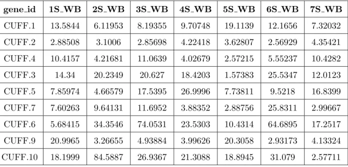
The same pipeline to analyze the RNA-Seq data from Trapnell et al. [78] was used. Since the samples are paired-end, in TopHat, the strand-specific RNA-Seq protocol for sequence alignment was followed. After running TopHat, Cufflinks (version 2.1.1) was used here to quantify transcript counts. The Cufflinks suite uses the FPKM (Fragments Per Kilobase Million) normalization method to express transcript levels. The output folder contained the FPKM-tracking files of gene-level, transcripts, and isoforms with confidence. Then the FPKM tracking files from the Cufflinks output were merged to obtain the expression levels of all samples (see e.g. Table 3.1). In Figure 3.3, the mean sorted log distribution ofDrosophila melanogaster gene expression data is summarized.

A Linux server (OS) was used for preprocessing the Drosophila melanogaster dataset. Sample code is provided in the appendix section.

Table 3.1: A small subset of the gene expression data from theDrosophila melanogaster dataset.

gene id

1S WB

2S WB

3S WB

4S WB

5S WB

6S WB

7S WB

CUFF.1

13.5844

6.11953

8.19355

9.70748

19.1139

12.1656

7.32032

CUFF.2

2.88508

3.1006

2.85698

4.22418

3.62807

2.56929

4.35421

CUFF.4

10.4157

4.21681

11.0639

4.02679

2.57215

5.55237

10.4282

CUFF.3

14.34 20.2349

20.627 18.4203

1.57383

25.5347

12.0123

CUFF.5

7.85974

4.66579

17.5395

26.9996

7.73811

9.5218

16.8399

CUFF.7

7.60263

9.64131

11.6952

3.88352

2.88756

25.8311

2.99667

CUFF.6

5.68415

34.3546

74.0531

23.5303

10.4314

64.6895

17.2517

CUFF.9

20.9965

3.26655

4.93884

3.99626

20.3058

2.93173

4.13324

CUFF.10

18.1999

84.5887

26.9367

21.3088

18.8945

31.079 2.57711

3.3 Cluster comparison metric

Cluster comparison methods can compare two clusterings generated by a given algorithm. Such a method of comparison can answer the question of how much the clusterings can change when using different subsets of the samples to construct them. In this section, a cluster comparison metric is described, as well as three

Sample Size Evaluation and Comparison of K-Means Clusterings of RNA-Seq Gene Expression Data