Open Access
Research article
Evaluation of normalization methods for cDNA microarray data by
k
-NN classification
Wei Wu*
1,2, Eric P Xing
3, Connie Myers
1, I Saira Mian
1and Mina J Bissell
1Address: 1Life Sciences Division, Lawrence Berkeley National Laboratory, Berkeley, CA 94720, USA, 2Dorothy P. and Richard P. Simmons Center for Interstitial Lung Disease, Division of Pulmonary, Allergy and Critical Care Medicine, University of Pittsburgh Medical Center, Pittsburgh, PA 15213, USA and 3Center for Automated Learning and Discovery and Language Technology Institute, School of Computer Science, Carnegie Mellon University, Pittsburgh, PA 15213, USA
Email: Wei Wu* - [email protected]; Eric P Xing - [email protected]; Connie Myers - [email protected]; I Saira Mian - [email protected]; Mina J Bissell - [email protected]
* Corresponding author
Abstract
Background: Non-biological factors give rise to unwanted variations in cDNA microarray data. There are many normalization methods designed to remove such variations. However, to date there have been few published systematic evaluations of these techniques for removing variations arising from dye biases in the context of downstream, higher-order analytical tasks such as classification.
Results: Ten location normalization methods that adjust spatial- and/or intensity-dependent dye biases, and three scale methods that adjust scale differences were applied, individually and in combination, to five distinct, published, cancer biology-related cDNA microarray data sets. Leave-one-out cross-validation
(LOOCV) classification error was employed as the quantitative end-point for assessing the effectiveness of
a normalization method. In particular, a known classifier, k-nearest neighbor (k-NN), was estimated from data normalized using a given technique, and the LOOCV error rate of the ensuing model was computed. We found that k-NN classifiers are sensitive to dye biases in the data. Using NONRM and GMEDIAN as baseline methods, our results show that single-bias-removal techniques which remove either spatial-dependent dye bias (referred later as spatial effect) or intensity-spatial-dependent dye bias (referred later as intensity effect) moderately reduce LOOCV classification errors; whereas double-bias-removal techniques which remove both spatial- and intensity effect reduce LOOCV classification errors even further. Of the 41 different strategies examined, three two-step processes, IGLOESS-SLFILTERW7, ISTSPLINE-SLLOESS and IGLOESS-SLLOESS, all of which removed intensity effect globally and spatial effect locally, appear to reduce LOOCV classification errors most consistently and effectively across all data sets. We also found that the investigated scale normalization methods do not reduce LOOCV classification error.
Conclusion: Using LOOCV error of k-NNs as the evaluation criterion, three double-bias-removal normalization strategies, IGLOESS-SLFILTERW7, ISTSPLINE-SLLOESS and IGLOESS-SLLOESS, outperform other strategies for removing spatial effect, intensity effect and scale differences from cDNA microarray data. The apparent sensitivity of k-NN LOOCV classification error to dye biases suggests that this criterion provides an informative measure for evaluating normalization methods. All the computational tools used in this study were implemented using the R language for statistical computing and graphics.
Published: 26 July 2005
BMC Bioinformatics 2005, 6:191 doi:10.1186/1471-2105-6-191
Received: 17 December 2004 Accepted: 26 July 2005 This article is available from: http://www.biomedcentral.com/1471-2105/6/191
© 2005 Wu et al; licensee BioMed Central Ltd.
This is an Open Access article distributed under the terms of the Creative Commons Attribution License (http://creativecommons.org/licenses/by/2.0), which permits unrestricted use, distribution, and reproduction in any medium, provided the original work is properly cited.
Background
Molecular profiling technology allows for the simultane-ous assaying of the abundance of tens of thsimultane-ousands of transcripts in a biological sample. Once these abundance values have been obtained for many samples, prevalent higher-order data analyses may include clustering, classi-fication, feature selection, and network estimation. A vari-ety of algorithms seeking to address these higher-order tasks have been investigated and applied, to interpret gene expression patterns and to generate biological predic-tions. However, the accuracy of these predictions may depend on the low-level transformations utilized to pro-duce abundance values from raw measurements, i.e., data pre-processing may be a critical factor in determining the validity and success of downstream studies. Some key pre-processing steps for profiling data include image quantifi-cation and normalization. Several image analysis software (e.g., GenePix and SPOT) have been designed for image analysis of the spots on microarrays [1,2]. Background estimation has also been considered as an important issue in image quantification, however, evidence [2,3] showed that 'inappropriate' local background adjustment could add noise into the microarray data and thus be detrimen-tal to the downstream studies. Background adjustment, therefore, is still an issue to be resolved. After image anal-ysis, normalization usually needs to be performed. It is a procedure designed to minimize the unwanted variations in measurements arising from the technology, but to retain the intrinsic biological variations, and is also the focus of this work. In this study, we examined normaliza-tion in the context of a particular transcripnormaliza-tional profiling platform, cDNA microarrays [4-6], and the specific analyt-ical task of classifying biologanalyt-ical samples characterized by gene expression profiles.
In cDNA microarray-based investigations, RNA from two samples are reverse-transcribed and labeled with distinct (red and green) fluorescent dyes, then hybridized to a microarray spotted with DNA sequences ("probes"). An ensuing scanned image of the microarray is processed to yield an intensity measurement for each dye at every spot (Figure 1). If R and G are the spot-specific, quantitated, fluorescent intensities of the target and reference expres-sion signals respectively, relative gene expresexpres-sion is defined as the log ratio M = log2(R / G), and average
expression is the log intensity . Based on
different biological assumptions and design principles, many normalization methods for cDNA microarray data have been proposed. Global normalization techniques adjust the center (e.g., mean or median) of the distribu-tion of the log ratio M values on each microarray to a con-stant [1,7-9]. These methods, however, do not correct for any intensity- or spatial effect.
A variety of techniques have been proposed to remove intensity effect. A non-linear approach employs robust locally weighted regression (lowess) [10] to smooth the dependence of log ratios on intensities [4,11,12]. The basic assumption of this approach is either that the major-ity of genes are not differentially expressed, or that genes are influenced by random effects (i.e., the numbers of up-regulated and down-up-regulated genes are similar) [4,11,12]. A 'qspline' method uses a target array to adjust R and G values so that their distribution is similar for all arrays [13], but the performance of this method may depend upon the choice of the baseline array [14]. A com-posite method employs both external control samples and total genes on a microarray to remove intensity effect [15]. To relax critical biological assumptions, 'housekeep-ing-gene'-related methods first identify non-differentially-expressed genes, and then use these genes for normaliza-tion [16-18]. Semi-linear models are designed to account for the effects of print-tips (PTs), signal intensity, and
A=log2 RG
A scanned image of an illustrative cDNA microarray
Figure 1
A scanned image of an illustrative cDNA microarray. The configuration (layout of spots) can be described via a previously defined notation encompassing four numbers (ngr, ngc, nsr, nsc) [12]. A print-tip (PT) group is a set of spots arranged in a grid with "nsr" rows and "nsc" columns. A microarray is a set of PT groups arranged in a pattern of "ngr" rows and "ngc" columns. The configuration of the microarray shown is (ngr = 2, ngc = 2, nsr = 24, nsc = 24), i.e., 2 × 2 PT groups each composed of 24 × 24 spots. The terms "local" and "global" level refer to the spots in a PT group and the entire microarray respectively.
differences in gene expression levels jointly in a single model [19,20].
The removal of intensity effect at the PT level can partially remove spatial effect [4,11]. To remove spatial effect more completely, the dependence of M values on physical posi-tion can be smoothed using lowess [12], or can be elimi-nated using weighted mean [13] or median filter methods [17], both of which assume that differentially expressed genes are not co-localized in the neighboring spots. Since spatial- and intensity effect may be mutually dependent, a method that removes global spatial effect and global intensity effect in a single step has been proposed [21]. Whereas the above location normalization methods remove spatial- and intensity effect, scale normalization methods adjust differences in the scale of M values within and/or between microarrays. The assumption is that since the majority of genes are not differentially expressed, the scale of their M values should be constant. A robust esti-mate of the scale factor for scale normalization is median absolute deviation [15].
Normalization approaches seek to ensure that dye effect is removed, while biological variations are retained. Spatial-and intensity effect Spatial-and scale effect arise from printing, hybridization, scanning, or other technical factors, and can mask the signals arising from genuine biological vari-ations in gene expression. Visual aids used to assess the effectiveness of normalization methods [11,13,15,21] include scatter plots of log ratio (M) versus average log intensity (A) ("MA plots"). Spatial plots are a color-coded representation of each spot on a microarray that depicts M values, or a quality (e.g., shape, size) measure of some test statistic. These two types of diagnostic plots [4,21] suggest that raw M values are often biased estimates of relative expression and that the dye intensities per spot need to be adjusted. Quantitative criteria used to assess the robust-ness of normalization methods in removing dye effect include (i) rank variations of spot intensity in non-nor-malized versus nornon-nor-malized data [9,22], and (ii) correla-tion [16,21], variance [8,13], or error [18,22] of the normalized M values in replicated data.
To ensure that biological variations are retained after nor-malization, several functional criteria have been employed. Prevailing approaches determine the ability to predict a fixed number of differentially expressed genes in real or simulated data using quantitative measures based on t-statistics [4,11,13,21], adjusted p-values [11], and false-discovery rates [23]. However, there is uncertainty associated with these measures, and the true number of differentially expressed genes is unknown. Spike-in data have been used to assess normalization approaches for Affymetrix GeneChip data [14,24,25]. However, external
control samples are not widely used for evaluation of nor-malization methods for cDNA microarrays.
In this paper, we evaluated normalization methods for cDNA microarray data using the k-NN LOOCV classifica-tion error (of biological samples characterized by the gene expression profiles), an alternative quantitative functional measure that is relatively unambiguous, objective and readily computed. We used k-NN classifiers because (i) their sensitivity enables us to discriminate between, and hence evaluate normalization techniques, (ii) they are readily available, (iii) they perform well in practice, and (iv) their non-parametric nature means that assumptions about how the data are distributed have little influence on classification performance. Since the primary aim of our evaluation of normalization methods was to assist practi-tioners in choosing effective data pre-processing schemes, we did not consider factors that may influence classifica-tion performance, such as feature selecclassifica-tion and distance metrics. We investigated a wide spectrum of well-known and widely available normalization techniques: ten loca-tion normalizaloca-tion methods that adjust spatial effect and/ or intensity effect (Table 1), and three scale methods that adjust scale differences (Table 3). We applied these meth-ods, individually and in combination (41 strategies in all, Tables 1, 2, 3), to five diverse, published, cancer biology-related cDNA microarray data sets (Table 4), and we gen-erated data sets with spatial effect, intensity effect and scale differences removed to varying degrees. Computing
the LOOCV classification error of k-NNs estimated from
these multi- and two-class data sets allowed us to investi-gate which and how much of the dye effect are removed by the 41 strategies.
Results
Spatial- and intensity-dependent normalization Diagnostic plots
We used diagnostic plots to examine the ability of differ-ent location normalization methods to remove spatial-and/or intensity effect (Tables 1 and 2). Figure 2 shows spatial plots for two specific LYMPHOMA microarrays normalized with four approaches designed to correct spa-tial effect (SLLOESS, SLFILTERW3, SLFILTERW7, IG
S-GLOESS). The non-normalized M values (NONRM) for microarray "5850" display global spatial effect (left-to-right, green-to-red pattern) whereas those for microarray "5938" exhibit local spatial effect (top-to-bottom, green-to-red pattern in each PT group). Removal of spatial effect should result in a "random" red and green pattern of M values. SLLOESS and SLFILTERW7 exhibit similar dye bias-removal abilities in that they both remove global spa-tial effect more effectively than local spaspa-tial effect. SLFILTERW3 removes both global and local dye effect effectively, largely because it uses a median filter of a small window size (3 × 3 spots) for normalization. IGSGLOESS
removes most, but not all, global and local spatial effect (a strip of red spots on the right side of "5850" and on the bottom of the PT groups in the first row of "5938" remain). IGSGLOESS may not be as effective at removing dye effect as expected because, as the developers indicate,
lowess curve construction uses the standardized spatial variables (rloc, cloc), which may not be appropriate for location variables [21].
Figure 3 shows intensity-dependent MA plots for one spe-cific LYMPHOMA microarray overlaid with one lowess
curve (left) or one lowess curve per print tip group (right) using six methods designed to correct intensity effect (IGLOESS, ILLOESS, ISTSPLINE, QSPLINEG, QSPLINER, IGSGLOESS). For non-normalized M values (NONRM), the curvature in the MA plot indicates the presence of intensity effect at the array (left) and PT (right) level. All six methods remove global intensity effect completely
(flat lowess curves, left), but only ILLOESS and IG
S-GLOESS remove local intensity effect thoroughly (right). Visual inspection of the diagnostic plots in Figures 2 and 3 suggest that SLFILTERW3 is an effective method for removing both global and local spatial effect, whereas ILLOESS is good at removing intensity effect.
k-NN LOOCV Classification error
For a functional, quantitative evaluation of location nor-malization methods, we first computed k-NN LOOCV classification error rates for data normalized using these methods individually and/or in combination. Then for each data set, we ranked the normalization methods based on their LOOCV classification error rates. The smaller the LOOCV classification error rate, the lower the rank of the normalization strategy. In order to assess whether normalization is beneficial (or not), we also
Table 1: Single-bias-removal location normalization techniques used in this study. These strategies remove spatial- or intensity effect in a single step. The abbreviations are as follows, (for a given microarray), Ml: location-normalized log ratio; median(M): median value of non-normalized log ratios; lowess(rloci, cloci): lowess curve fitted as a function of the row location (rloci) and column location (cloci) of spots in PT group i; median(Mw): median value of non-normalized log ratios within the window size determined by w; lowess(A): lowess curve fitted to an MA plot of spots on a microarray; lowess(Ai): lowess curve fitted to an MA plot of spots in PT group i;
spline(Aiset): spline curve fitted to an MA plot of spots in the invariant set, iset; Rl: location-normalized R value; qspline(Gi): qspline smoothing using geometric mean of the G channels of all arrays as a target array; Gl: location-normalized G value; qspline(Rt): qspline smoothing using geometric mean of the R channels of all arrays as a target array.
Name * Description: Effect/Level Bioconductor R package/function(parameters)
NONRM No normalization Ml = M marray/maNorm(norm="none")
GMEDIAN Global Ml = M - median(M) marray/maNorm (norm="median", subset = T)
SLLOESS Spatial/local lowess Ml = M - loess(rloci, cloci) marray/maNormMain (f.loc = list(maNorm2D(g="maPrintTip", subset = T, span = 0.4))
SLFILTERW3 Spatial/Local median filter Ml = M - median(Mw), W = 3 × 3
tRMA/SpatiallyNormalise** (M, width = 3, height = 3) SLFILTERW7 Spatial/Local median filter
Ml = M - median(Mw), W = 7 × 7
tRMA/SpatiallyNormalise** (M, width = 7, height = 7) IGLOESS Intensity/Global lowess Ml = M - loess(A) marray/maNorm (norm="loess", subset = TRUE, span = 0.4)
ILLOESS Intensity/Local lowess Ml = M - loess(Ai) marray/maNorm (norm="printTipLoess", subset = T, span = 0.4) ISTSPLINE Intensity/Global spline Ml = M - spline(Aiset) affy/normalize.invariantset**(prd.td = c(0.003, 0.007))
QSPLINEG Intensity/Global qspline
Rl = R - qspline(Gt), Gl = G - qspline(Gt), Ml = log(Rl / Gl)
affy/Rl ← normalize.qspline(R, 2^rowMeans(log2(G), na.rm = T), na.rm = T, *default*)
Gl ← normalize.qspline(G, 2^rowMeans(log2(G), na.rm = T), na.rm = T, *default*)
QSPLINER Intensity/Global qspline
Rl = R - qspline(Rt), Gl = G - qspline(Rt), Ml = log(Rl / Gl)
affy/ Rl ← normalize.qspline(R, 2^rowMeans(log2(R), na.rm = T), na.rm = T, *default*)
Gl ← normalize.qspline(G, 2^rowMeans(log2(R), na.rm = T), na.rm = T, *default*)
* We adopted the terminology given in the table to avoid confusion within this work. Elsewhere, these methods are known as: GMEDIAN, global or median [4]; SLLOESS, 2D spatial [12]; SLFILTERW3, spatial normalization using median filter of the block size 3 × 3 [17]; SLFILTERW7, spatial normalization using median filter of the block size 7 × 7 [17]; IGLOESS, global loess [4, 26]; ILLOESS, print-tip loess [4]; ISTSPLINE, invariant set normalization [38]; QSPLINER, qspline using geometric mean of the R channels of all arrays as the target array [13]; QSPLINEG, qspline using geometric mean of the G channels of all arrays as the target array [13].
** The SpatiallyNormalise function in the tRMA package was modified to remove scale normalization. The normalize.invariantset function in Affy package was modified so that the function could be applied on cDNA microarray data.
*default* The default parameters for QSPLINEG and QSPLINER are (fit.iters = 5, min.offset = 5, spline.method="natural", smooth = T, spar = 0, p.min = 0, p.max = 1.0, incl.ends = T, converge = F)
computed the following quantity for a normalization method in each data set:
IMPROVEMENT = (ErrorRate(NONRM) -
Error-Rate(Method)) / ErrorRate(NONRM) × 100%
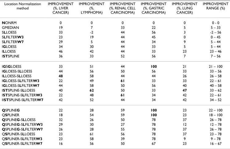
where ErrorRate(NONRM) is the error rate of NONRM, and ErrorRate(Method) is the error rate of the method. Tables 5 and 6 give results for five data sets (Table 4) and 23 location methods designed to remove spatial- and/or intensity effect (Tables 1 and 2). Figures 4 and 5 are alter-native, visual representations of the classification "Error Rate" and "Rank" in Table 5.
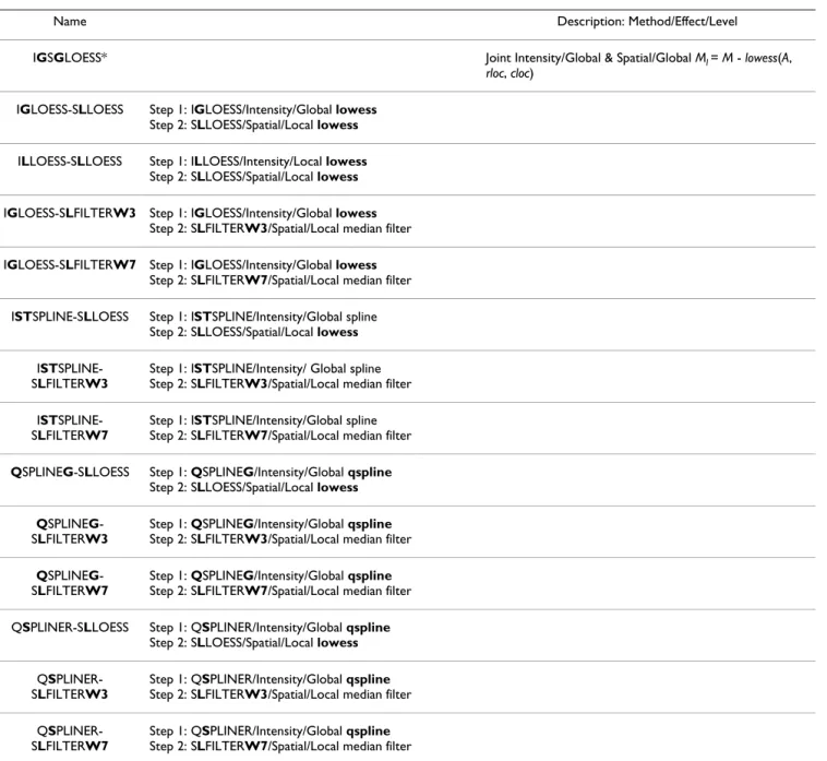
Table 2: Double-bias-removal location normalization techniques used in this study. These strategies remove both spatial- and intensity effect either in a single step (IGSGLOESS) or in two steps (the remaining thirteen approaches) by combining methods listed in Table 1.
Name Description: Method/Effect/Level
IGSGLOESS* Joint Intensity/Global & Spatial/Global Ml = M - lowess(A,
rloc, cloc) IGLOESS-SLLOESS Step 1: IGLOESS/Intensity/Global lowess
Step 2: SLLOESS/Spatial/Local lowess ILLOESS-SLLOESS Step 1: ILLOESS/Intensity/Local lowess
Step 2: SLLOESS/Spatial/Local lowess IGLOESS-SLFILTERW3 Step 1: IGLOESS/Intensity/Global lowess
Step 2: SLFILTERW3/Spatial/Local median filter IGLOESS-SLFILTERW7 Step 1: IGLOESS/Intensity/Global lowess
Step 2: SLFILTERW7/Spatial/Local median filter ISTSPLINE-SLLOESS Step 1: ISTSPLINE/Intensity/Global spline
Step 2: SLLOESS/Spatial/Local lowess IST
SPLINE-SLFILTERW3
Step 1: ISTSPLINE/Intensity/ Global spline Step 2: SLFILTERW3/Spatial/Local median filter IST
SPLINE-SLFILTERW7
Step 1: ISTSPLINE/Intensity/Global spline Step 2: SLFILTERW7/Spatial/Local median filter QSPLINEG-SLLOESS Step 1: QSPLINEG/Intensity/Global qspline
Step 2: SLLOESS/Spatial/Local lowess QSPLINEG
-SLFILTERW3
Step 1: QSPLINEG/Intensity/Global qspline Step 2: SLFILTERW3/Spatial/Local median filter QSPLINEG
-SLFILTERW7
Step 1: QSPLINEG/Intensity/Global qspline Step 2: SLFILTERW7/Spatial/Local median filter QSPLINER-SLLOESS Step 1: QSPLINER/Intensity/Global qspline
Step 2: SLLOESS/Spatial/Local lowess QS
PLINER-SLFILTERW3
Step 1: QSPLINER/Intensity/Global qspline Step 2: SLFILTERW3/Spatial/Local median filter QS
PLINER-SLFILTERW7
Step 1: QSPLINER/Intensity/Global qspline Step 2: SLFILTERW7/Spatial/Local median filter * IGSGLOESS was implemented in the following package/function: MAANOVA R package/smooth (method="rlowess", f = 0.4, degree = 2). Elsewhere, IGSGLOESS is known as joint loess [21]. lowess(A, rloc, cloc): lowess curve fitted as a function of average log intensity (A), row location (rloc), and column location (cloc) of spots on a microarray.
Single-bias-removal methods
These strategies can be classified into two categories, spa-tial-dependent and intensity-dependent normalization methods. Three spatial-dependent normalization meth-ods (SLLOESS, SLFILTERW3, SLFILTERW7) reduce k-NN
LOOCV classification error rates to a similar extent (Tables
5 and 6) and have almost identical ranks (Figure 5), despite the fact that their abilities to remove spatial effect are quite different (Figure 2). Since both SLLOESS and SLFILTERW7 fail to remove local spatial patterns effec-tively (Figure 2, rows 2 and 4), SLFILTERW3 may be too aggressive in removing "dye effect" (Figure 2, row 3). However, the three intensity-dependent methods (IGLOESS, ILLOESS, ISTSPLINE) reduce k-NN LOOCV classification error rates to different degrees. The k-NN
LOOCV classification error rate and rank of IGLOESS are
similar to those of the three spatial-dependent methods (SLLOESS, SLFILTERW3, SLFILTERW7) (Figure 5), whereas ILLOESS, which removes intensity effect more completely than IGLOESS, has smaller k-NN LOOCV clas-sification error rates than IGLOESS in all five data sets. ISTSPLINE, which uses a rank invariant set for
normaliza-tion, is also better than IGLOESS in all five data sets (Fig-ure 5).
In all five data sets, except for LYMPHOMA (SLLOESS), the single-bias-removal normalization methods consistently yield smaller LOOCV classification error rates than no-bias-removal methods, NONRM and GMEDIAN (which only sets the median of the distribution of M val-ues to zero). The greatest benefit, an IMPROVEMENT of 56%, is seen with GASTRIC CARCINOMA (SLLOESS, IST -SPLINE) (Table 6).
Double-bias-removal methods
IGSGLOESS removes both spatial- and intensity effect in one step, whereas the remaining seven approaches are two-step strategies consisting of single-bias-removal methods applied sequentially (first a method to remove intensity effect, followed by a method to remove spatial effect).
In general, double-bias-removal methods have smaller k
-NN LOOCV classification error rates and bigger
IMPROVEMENT than single-bias-removal methods, and
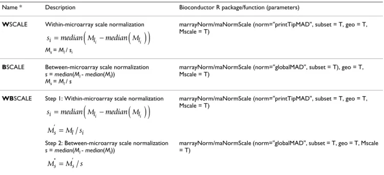
Table 3: Extant scale normalization techniques used in this study. For a given microarray, if Ml is a location-normalized log ratio, then
Ms is the scale-normalized log ratio, where Ms = Ml / s, and s is median absolute deviation from the median (MAD), a robust estimate of the scale of the data distribution. The remaining abbreviations are as follows, median(Ml): median value of Ml values of spots on all
microarrays in a data set; : median value of Ml values of spots in PT group i on a microarray.
Name * Description Bioconductor R package/function (parameters)
WSCALE Within-microarray scale normalization
Ms = Ml / si
marrayNorm/maNormScale (norm="printTipMAD", subset = T, geo = T, Mscale = T)
BSCALE Between-microarray scale normalization
s = median(Ml - median(Ml)) Ms = Ml / s
marrayNorm/maNormScale (norm="globalMAD", subset = T), geo = T, Mscale = T)
WBSCALE Step 1: Within-microarray scale normalization marrayNorm/maNormScale (norm="printTipMAD", subset = T, geo = T, Mscale = T)
Step 2: Between-microarray scale normalization s = median(Ml - median(Ml))
marrayNorm/maNormScale (norm="globalMAD", subset = T, geo = T, Mscale = T)
* We adopted the terminology given in this table to avoid confusion within this work. Elsewhere, the methods are known as: WSCALE, within-print-tip-group scale normalization [4]; and BSCALE, between slide scale normalization [4, 15].
median Ml i
( )
si median Ml median Ml i i =(
−( )
)
si median Ml median Ml i i =(
−( )
)
M’s =M sl/ i M"s =Ms’/sall perform better than NONRM and GMEDIAN (Tables 5 and 6, Figures 4 and 5). Using an arbitrary cut-off value of 10 for both median and upper quantile ranks (Figure 5), IGLOESS-SLFILTERW7, ISTSPLINE-SLLOESS and IGLOESS-SLLOESS (all of which remove intensity effect globally and then spatial effect locally) appear to be the best methods overall. These three two-step strategies not only have the lowest ranks amongst all normalization methods and across all data sets (Figure 5), they also showed most consistent and significant IMPROVEMENT over both NONRM and GMEDIAN across all five data sets (Table 6). The benefits of using IGLOESS-SLFILTERW7
over no normalization (NONRM) range from an IMPROVEMENT value of 40% in LUNG CANCER to 58% in LYMPHOMA (Table 6), whereas the IMPROVEMENT values of ISTSPLINE-SLLOESS range from 33% in GAS-TRIC CARCINOMA to 62% in LYMPHOMA and the IMPROVEMENT values of IGLOESS-SLLOESS range from 33% in LUNG CANCER to 56% in GASTRIC CARCINOMA.
The ranks of the SLFILTERW3-related approaches (IGLOESS-SLFILTERW3, ISTSPLINE-SLFILTERW3,
QSPLINEG-SLFILTERW3, QSPLINER-SLFILTERW3) are higher than their SLFILTERW7 counterparts (Figure 5), suggesting that a window size of 7 × 7 is more preferable than that of 3 × 3. A smaller window size may over nor-malize the data, and thus conceal real biological variations.
Compared to the two-step approaches, the rank of the one-step method, IGSGLOESS, is higher than IG LOESS-SLFILTERW7 and ISTSPLINE-SLLOESS (yet lower than IGLOESS-SLFILTERW3 and ISTSPLINE-SLFILTERW3). This indicates that the one-step IGSGLOESS has no appar-ent advantage over the two-step bias-removal strategies. Overall, the classification performances of data normal-ized using the double-bias-removal methods are better than that of NONRM, and the benefits (IMPROVEMENT) of doing so range from 21% in the case of LUNG CANCER
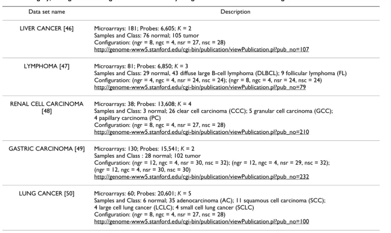
Table 4: The multi-class, cancer-biology related transcriptional profiling data sets analyzed in this work. For each of the five published studies, the fluorescent intensities, microarray images, and associated information were downloaded from the URLs indicated. The statistics refer to data sets produced after application of all pre-normalization data processing, location/scale normalization, and post-normalization data processing steps. The abbreviations are as follows, Microarrays: number of cDNA microarrays; Probes: number of probes; K: total number of categories to which a sample could be assigned; Samples and Class: number of samples in the specified pre-defined category; Configuration: configuration of a microarray using the convention described in Figure 1.
Data set name Description
LIVER CANCER [46] Microarrays: 181; Probes: 6,605; K = 2 Samples and Class: 76 normal; 105 tumor
Configuration: (ngr = 8, ngc = 4, nsr = 27, nsc = 28)
http://genome-www5.stanford.edu/cgi-bin/publication/viewPublication.pl?pub_no=107
LYMPHOMA [47] Microarrays: 81; Probes: 6,850; K = 3
Samples and Class: 29 normal, 43 diffuse large B-cell lymphoma (DLBCL); 9 follicular lymphoma (FL) Configuration: (ngr = 4, ngc = 4, nsr = 24, nsc = 24); (ngr = 8, ngc = 4, nsr = 24, nsc = 24) http://genome-www5.stanford.edu/cgi-bin/publication/viewPublication.pl?pub_no=79 RENAL CELL CARCINOMA
[48]
Microarrays: 38; Probes: 13,608; K = 4
Samples and Class: 3 normal; 26 clear cell carcinoma (CCC); 5 granular cell carcinoma (GCC); 4 papillary carcinoma (PC)
Configuration: (ngr = 8, ngc = 4, nsr = 27, nsc = 28)
http://genome-www5.stanford.edu/cgi-bin/publication/viewPublication.pl?pub_no=210 GASTRIC CARCINOMA [49] Microarrays: 130; Probes: 15,541; K = 2
Samples and Class : 28 normal; 102 tumor
Configuration: (ngr = 12, ngc = 4, nsr = 30, nsc = 32); (ngr = 12, ngc = 4, nsr = 29, nsc = 32); (ngr = 12, ngc = 4, nsr = 30, nsc = 30)
http://genome-www5.stanford.edu/cgi-bin/publication/viewPublication.pl?pub_no=232
LUNG CANCER [50] Microarrays: 60; Probes: 20,601; K = 5
Samples and Class: 6 normal; 35 adenocarcinoma (AC); 11 squamous cell carcinoma (SCC); 4 large cell lung cancer (LCLC); 4 small cell lung cancer (SCLC)
Configuration: (ngr = 8, ngc = 4, nsr = 27, nsc = 28)
(IGSGLOESS) to 100% in GASTRIC CARCINOMA (IG
S-GLOESS) (Table 6). Qspline-related approaches
Unlike the location normalization methods discussed above, qspline-related approaches require a target array.
QSPLINEG and QSPLINER are single-bias-removal tech-niques and use G and R respectively as the target array. The reduction in k-NN LOOCV classification error rates for these methods is quite significant compared to the other single-bias-removal methods. However, it is noticeable that although QSPLINEG and QSPLINER produce similar results in almost all data sets, their results are different in LYMPHOMA (Figures 4 and 5). In addition, when
QSPLINEG or QSPLINER is combined with one of the three spatial-dependent methods, the rank of the resulting double-bias-removal technique is different from that of its counterpart technique (Figure 5). These results suggest that, similar to other baseline array-based normalization methods [14], the performances of the qSpline-related methods may also depend on the choice of the target array.
Overall, the classification performance of data normal-ized using the qspline-related methods is better than
NONRM by IMPROVEMENT values of 9% in LUNG CAN-CER (QSPLINER-SLFILTERW3) and of 100% in GASTRIC CARCINOMA (QSPLINEG, QSPLINER). None of these
qSpline-related methods, however, outperforms the IGLOESS-SLFILTERW7 (Table 6).
Scale normalization
Figure 6 shows boxplots of the distribution of non-nor-malized M values for microarrays in the five studies. Scale effect is more apparent between (right) rather than within (left) microarrays in a study. The LYMPHOMA data set shows considerable variations in box size and whisker length both within and between microarrays.
1 2 3 4 4 3 2 1 −4 −2 0 2 4 Nonorm: 5850 1 2 3 4 4 3 2 1 −4 −2 0 2 4 Nonorm: 5938 1 2 3 4 4 3 2 1 −4 −2 0 2 4 sLloess: 5850 1 2 3 4 4 3 2 1 −4 −2 0 2 4 sLloess: 5938 1 2 3 4 4 3 2 1 −4 −2 0 2 4 sLfilterW3: 5850 1 2 3 4 4 3 2 1 −4 −2 0 2 4 sLfilterW3: 5938 1 2 3 4 4 3 2 1 −4 −2 0 2 4 sLfilterW7: 5850 1 2 3 4 4 3 2 1 −4 −2 0 2 4 sLfilterW7: 5938 1 2 3 4 4 3 2 1 −4 −2 0 2 4 iGsGloess: 5850 1 2 3 4 4 3 2 1 −4 −2 0 2 4 iGsGloess: 5938
Spatial plots of microarrays 5850 and 5938 in the Lymphoma data set
Figure 2
Spatial plots of microarrays 5850 and 5938 in the Lymphoma data set. Spatial plots of microarrays 5850 and 5938 in the LYMPHOMA data set. The plots show the results before and after location normalization designed to remove spatial effect. The spatial plot is a spatial representa-tion of spots on the microarray color-coded by their M val-ues (marrayPlots/maImage(x="maM", subset = T)). Spots in white are spots flagged in the original microarray data (missing values). Rows depict non-normalized (NONRM), and normalized Ml values (SLLOESS, SLFILTERW3, SLFILTERW7, IGSGLOESS).
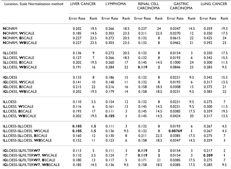
Tables 7 and 8 and Figure 7 show LOOCV classification error rates, ranks and IMPROVEMENT for the k-NN clas-sifiers estimated using 3 scale normalization methods combined with other spatial- and/or intensity-dependent normalization methods (18 strategies in all). For data normalized first with spatial- and/or intensity-dependent methods, little or no reduction in LOOCV classification error rates was observed when within-microarray scale normalization (WSCALE) was applied later. However, when between-microarray scale normalization (BSCALE) was used alone, or when both scale normalization tech-niques were used sequentially (WBSCALE), there was an increase in both median and upper quantile ranks (Figure 7), suggesting that BSCALE should not be applied on the studied data sets. With regard to our running example, the LYMPHOMA data set, scale normalization has no appar-ent beneficial effect on classification performance.
Discussion
This computational investigation employed two types of visual diagnostic plots and k-NN LOOCV classification error rates to evaluate a broad suite of known normaliza-tion strategies. These analyses were applied to cDNA microarray data from five published cancer studies. Since all these data sets were acquired using GenePix image analysis software and a recent study showed that back-ground adjustment using GenePix can increase variability of microarray data and compromise downstream data analyses [3], we used foreground intensity values of the probes without background adjustment in this work. The normalization approaches examined are based on a vari-ety of different techniques and implementations that are readily available and accessible.
6 8 10 12 14 Ŧ 4 Ŧ 2 024 A M Nonorm 6 8 10 12 14 Ŧ 4 Ŧ 2 024 A M Nonorm 6 8 10 12 14 Ŧ 4 Ŧ 2 024 A M iGloess 6 8 10 12 14 Ŧ 4 Ŧ 2 024 A M iGloess 6 8 10 12 14 Ŧ 4 Ŧ 2 024 A M iLloess 6 8 10 12 14 Ŧ 4 Ŧ 2 024 A M iLloess 6 8 10 12 14 Ŧ 4 Ŧ 2 024 A M iSTspline 6 8 10 12 14 Ŧ 4 Ŧ 2 024 A M iSTspline 6 7 8 9 10 11 12 13 Ŧ 4 Ŧ 2 024 A M qsplineG 6 7 8 9 10 11 12 13 Ŧ 4 Ŧ 2 024 A M qsplineG 6 7 8 9 10 11 12 13 Ŧ 4 Ŧ 2 024 A M qsplineR 7 8 9 10 11 12 13 Ŧ 4 Ŧ 2 024 A M qsplineR 6 8 10 12 14 Ŧ 4 Ŧ 2 024 A M iGsGloess 6 8 10 12 14 Ŧ 4 Ŧ 2 024 A M iGsGloess
MA plots of microarray 5812 in the LYMPHOMA data set
Figure 3
MA plots of microarray 5812 in the LYMPHOMA data set. The plots show the results before and after loca-tion normalizaloca-tion designed to remove intensity effect. The MA plot is a scatter plot of log ratio M = log2(Rf / Gf) (abscissa) versus average log intensity
(ordinate). Columns depict non-normalized (NONRM), and normalized Ml values (IGLOESS, ILLOESS, ISTSPLINE,
QSPLINEG, QSPLINER, IGSGLOESS). Plots in the same row represent same data except that each plot in the left panel shows one lowess curve for all the spots ( marray-Plots/maPlot(data, z = NULL)); while that in the right panel shows one lowess curve per PT group (marrayPlots/ maPlot(x="maA", y="maM", z="maPrintTip")). Dif-ferent colors and line types are used to represent difDif-ferent groups from different rows ("ngr", Figure 1) and columns ("ngc") respectively.
Our results show that the LOOCV classification error of k -NN classifiers depends on how much of spatial- and intensity effect can be removed by a normalization strat-egy. Overall, the single-bias-removal location approaches perform better than GMEDIAN and NONRM, while the double-bias-removal location strategies perform better than the single-bias-removal location approaches. Of the twenty-three location normalization techniques investi-gated, three two-step processes (IGLOESS-SLFILTERW7, ISTSPLINE-SLLOESS and IGLOESS-SLLOESS), all of which removes intensity effect at the global level and spa-tial effect at the local level, appear to be the most effective at reducing LOOCV classification error. However, remov-ing spatial- or intensity effect alone is not sufficient for reducing LOOCV classification error (see below).
A recent review of normalization methods [26] raised the concern that removing spatial effect (SLLOESS and the related methods) may add additional noise to normalized
data, and suggested that a safe alternative was removing only intensity effect at the local level (ILLOESS) [26]. Our results show that, although the classification performance of data normalized with SLLOESS alone can be worse than non-normalized data as in the case of the LYM-PHOMA data set, when SLLOESS is combined with another intensity-dependent approach (IGLOESS, ILLOESS, ISTSPLINE, QSPLINEG, or QSPLINER), there is
considerable improvement over NONRM, with
IMPROVEMENT ranging from 23% in LIVER CANCER (QSPLINER-SLLOESS) to 78% in GASTRIC CARCINOMA (QSPLINER-SLLOESS, QSPLINEG-SLLOESS). Thus, removing both spatial- and intensity effect is beneficial for the downstream analytical task of classification. Another study compared various lowess-based single-bias-removal intensity normalization approaches, and found that ILLOESS may not significantly improve the results compared to IGLOESS [27]. Our results show that the benefits (IMPROVEMENT) of IGLOESS over NONRM
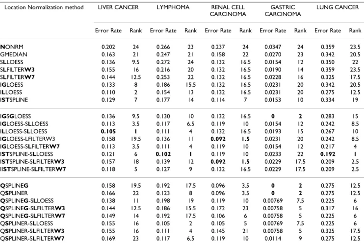
Table 5: Leave-one-out cross-validation k-NN error rates for location normalized data. For each data set, the normalization methods were ranked based on their LOOCV classification error rates ("Rank"). The smaller the LOOCV classification error rate, the lower the rank. The methods are arranged in the following order: single-bias-removal methods (block 1), double-bias-removal methods (block 2) and the qspline-related methods (block 3). For a given data set, the smallest error rate(s) and rank(s) are shown in bold. The methods and data sets are described in Tables 1, 2 and 4, respectively.
Location Normalization method LIVER CANCER LYMPHOMA RENAL CELL
CARCINOMA
GASTRIC CARCINOMA
LUNG CANCER
Error Rate Rank Error Rate Rank Error Rate Rank Error Rate Rank Error Rate Rank
NONRM 0.202 24 0.266 23 0.237 24 0.0347 24 0.359 23.5 GMEDIAN 0.163 21 0.247 21 0.158 22 0.0270 23 0.342 20.5 SLLOESS 0.136 9.5 0.272 24 0.132 16.5 0.0154 12 0.350 22 SLFILTERW3 0.155 16 0.216 20 0.132 16.5 0.0190 14 0.359 23.5 SLFILTERW7 0.144 12.5 0.253 22 0.132 16.5 0.0228 16 0.325 17.5 IGLOESS 0.133 8 0.186 15.5 0.132 16.5 0.0231 20 0.342 20.5 ILLOESS 0.110 2 0.154 13 0.132 16.5 0.0231 20 0.275 12.5 ISTSPLINE 0.129 7 0.177 14 0.114 7 0.0153 10 0.334 19 IGSGLOESS 0.136 9.5 0.130 10 0.132 16.5 0 2 0.283 15 IGLOESS-SLLOESS 0.113 3.5 0.117 6.5 0.119 10 0.0154 12 0.242 8.5 ILLOESS-SLLOESS 0.105 1 0.111 4 0.132 16.5 0.0193 15 0.267 10 IGLOESS-LFILTERW3 0.158 19.5 0.136 11 0.092 1.5 0.0231 20 0.242 8.5 IGLOESS-SLFILTERW7 0.113 3.5 0.111 4 0.119 10 0.0154 12 0.217 4 ISTSPLINE-SLLOESS 0.121 6 0.102 1 0.119 10 0.0233 22 0.192 1 ISTSPLINE-SLFILTERW3 0.157 18 0.139 12 0.092 1.5 0.0229 17.5 0.209 2.5 IISTSPLINE-SLFILTERW7 0.118 5 0.127 9 0.132 16.5 0.0229 17.5 0.209 2.5 QSPLINEG 0.158 19.5 0.192 17.5 0.096 3.5 0 2 0.275 12.5 QSPLINER 0.166 22 0.123 8 0.096 3.5 0 2 0.275 12.5 QSPLINEG-SLLOESS 0.138 11 0.198 19 0.119 10 0.00769 7.5 0.225 6 QSPLINEG-SLFILTERW3 0.144 12.5 0.186 15.5 0.172 23 0.00758 5 0.317 16 QSPLINEG-SLFILTERW7 0.149 14 0.192 17.5 0.106 6 0.00758 5 0.225 6 QSPLINER-SLLOESS 0.155 16 0.105 2 0.105 5 0.00769 7.5 0.225 6 QSPLINER-SLFILTERW3 0.155 16 0.111 4 0.145 21 0.00758 5 0.325 17.5 QSPLINER-SLFILTERW7 0.169 23 0.117 6.5 0.119 10 0.0114 9 0.275 12.5
range from 5% in LUNG CANCER to 44% in RENAL CELL CARCINOMA; while that the benefits (IMPROVEMENT) of ILLOESS over NONRM range from 23% in RENAL CELL CARCINOMA to 46% in LIVER CANCER. Therefore, ILLOESS performs better than IGLOESS in our study. However, as a single-bias-removal approach, ILLOESS still fail to outperform IGLOESS-SLFILTERW7, IST SPLINE-SLLOESS and IGLOESS-SLLOESS, which are the best over-all methods and whose IMPROVEMENT values over
NONRM range from 40% in LUNG CANCER to 58% in LYMPHOMA for IGLOESS-SLFILTERW7, from 33% in GASTRIC CARCINOMA to 62% in LYMPHOMA for IST -SPLINE-SLLOESS and from 33% in LUNG CANCER to 56% in GASTRIC CARCINOMA for IGLOESS-SLLOESS (Table 6).
A previous study employed k-NN classification of diluted samples to assess a small number of global linear meth-ods for normalization [28]. The study presented here is more comprehensive, both in terms of the range of data
sets and the diversity of normalization techniques. Our results indicate that the k-NN LOOCV classification error of real biological samples provides an informative functional quantitative measure that can be used to eval-uate normalization approaches.
Differences in scale between microarrays can arise from both unwanted technical factors (differences in experi-mental reagents, equipment, personnel, and so on), as well as from genuine biological variations. The scale nor-malization techniques applied here aim to remove unwanted technical factors, and assume the existence of little biological variations between samples. For the five studied data sets, scale normalization of non- or location-normalized data do not result in an overall reduction in
LOOCV classification error. Indeed, two
between-micro-array normalization methods (BSCALE, WBSCALE) result in an overall increase in LOOCV classification error (poorer performance, Figure 7). These results suggest that in the examined cancer-related data sets, there can be
con-Table 6: IMPROVEMENT of location normalization methods. IMPROVEMENT is defined (in the Results) based on improvement of
LOOCV classification error rate of a given normalization method over that of NONRM. The methods are arranged in the same order
as those in Table 5. For a given data set, the biggest IMPROVEMENT(s) is shown in bold. The methods and data sets are described in Tables 1, 2 and 4, respectively.
Location Normalization method IMPROVEMENT (%, LIVER CANCER) IMPROVEMENT (%, LYMPHOMA) IMPROVEMENT (%, RENAL CELL CARCINOMA) IMPROVEMENT (%, GASTRIC CARCINOMA) IMPROVEMENT (%, LUNG CANCER) IMPROVEMENT RANGE (%) NONRM 0 0 0 0 0 0 - 0 GMEDIAN 19 7 33 22 5 5 – 33 SLLOESS 33 -2 44 56 3 -2 – 56 SLFILTERW3 23 19 44 45 0 0 – 45 SLFILTERW7 29 5 44 34 9 5 – 44 IGLOESS 34 30 44 33 5 5 – 44 ILLOESS 46 42 44 33 23 23 – 46 ISTSPLINE 36 33 52 56 7 7 – 56 IGSGLOESS 33 51 44 100 21 21 – 100 IGLOESS-SLLOESS 44 56 50 56 33 33 – 56 ILLOESS-SLLOESS 48 58 44 44 26 26 – 58 IGLOESS-SLFILTERW3 22 49 61 33 33 22 – 61 IGLOESS-SLFILTERW7 44 58 50 56 40 40 – 58 ISTSPLINE-SLLOESS 40 62 50 33 47 33 – 62 ISTSPLINE-SLFILTERW3 22 48 61 34 42 22 – 61 IISTSPLINE-SLFILTERW7 42 52 44 34 42 34 – 52 QSPLINEG 22 28 59 100 23 22 – 100 QSPLINER 18 54 59 100 23 18 – 100 QSPLINEG-SLLOESS 32 26 50 78 37 26 – 78 QSPLINEG-SLFILTERW3 29 30 27 78 12 12 – 78 QSPLINEG-SLFILTERW7 26 28 55 78 37 26 – 78 QSPLINER-SLLOESS 23 61 56 78 37 23 – 78 QSPLINER-SLFILTERW3 23 58 39 78 9 9 – 78 QSPLINER-SLFILTERW7 16 56 50 67 23 16 – 67
Bar plots of leave-one-out cross-validation error rates for k-NNs in Table 5
Figure 4
Bar plots of leave-one-out cross-validation error rates for k-NNs in Table 5. The classifiers were estimated from five data sets (Table 4) either without normalization (NONRM) or normalized using twenty-three normalization techniques that remove spatial- and/or intensity effect to varying degrees (Tables 1 and 2). In each plot, the normalization methods are arranged in the following order: (A) Methods that remove no dye bias (GMEDIAN), or a single dye bias (SLLOESS, SLFILTERW3, SLFILTERW7, IGLOESS, ILLOESS, ISTSPLINE). (B) Methods that remove two dye biases (IGSGLOESS, IGLOESS-SLLOESS, ILLOESS-SLLOESS, IGLOESS-SLFILTERW3, IGLOESS-SLFILTERW7, ISTSPLINE-SLLOESS, IST SPLINE-SLFILTERW3, ISTSPLINE-SLFILTERW7). (C) Qspline-related methods (QSPLINEG, QSPLINER, QSPLINEG-SLLOESS, QSPLINEG-SLFILTERW3, QSPLINEG-SLFILTERW7, QSPLINER-SLLOESS, QSPLINER-SLFILTERW3, QS PLINER-SLFILTERW7).
Nonorm Gmedian sLloess sLfilterW3 sLfilterW7 iGloess iLloess iSTspline 0.00 0.05 0.10 0.15 0.20 0.25 (A) iGsGloess iGloess Ŧ sLloess iLloess Ŧ sLloess iGloess Ŧ sLfilterW3 iGloess Ŧ sLfilterW7 iSTspline Ŧ sLloess iSTspline Ŧ sLfilterW3 iSTspline Ŧ sLfilterW7 (B) QsplineG QsplineR QsplineG Ŧ sLloess QsplineG Ŧ sLfilterW3 QsplineG Ŧ sLfilterW7 QsplineR Ŧ sLloess QsplineR Ŧ sLfilterW3 QsplineR Ŧ sLfilterW7 (C) LiverCancer
Nonorm Gmedian sLloess sLfilterW3 sLfilterW7 iGloess iLloess iSTspline 0.00 0.05 0.10 0.15 0.20 0.25 0.30 (A) iGsGloess iGloess Ŧ sLloess iLloess Ŧ sLloess iGloess Ŧ sLfilterW3 iGloess Ŧ sLfilterW7 iSTspline Ŧ sLloess iSTspline Ŧ sLfilterW3 iSTspline Ŧ sLfilterW7 (B) QsplineG QsplineR QsplineG Ŧ sLloess QsplineG Ŧ sLfilterW3 QsplineG Ŧ sLfilterW7 QsplineR Ŧ sLloess QsplineR Ŧ sLfilterW3 QsplineR Ŧ sLfilterW7 (C) Lymphoma
Nonorm Gmedian sLloess sLfilterW3 sLfilterW7 iGloess iLloess iSTspline 0.00 0.05 0.10 0.15 0.20 0.25 (A) iGsGloess iGloess Ŧ sLloess iLloess Ŧ sLloess iGloess Ŧ sLfilterW3 iGloess Ŧ sLfilterW7 iSTspline Ŧ sLloess iSTspline Ŧ sLfilterW3 iSTspline Ŧ sLfilterW7 (B) QsplineG QsplineR QsplineG Ŧ sLloess QsplineG Ŧ sLfilterW3 QsplineG Ŧ sLfilterW7 QsplineR Ŧ sLloess QsplineR Ŧ sLfilterW3 QsplineR Ŧ sLfilterW7 (C) RenalCellCarcinoma
Nonorm Gmedian sLloess sLfilterW3 sLfilterW7 iGloess iLloess iSTspline 0.00 0.01 0.02 0.03 0.04 (A) iGsGloess iGloess Ŧ sLloess iLloess Ŧ sLloess iGloess Ŧ sLfilterW3 iGloess Ŧ sLfilterW7 iSTspline Ŧ sLloess iSTspline Ŧ sLfilterW3 iSTspline Ŧ sLfilterW7 (B) QsplineG QsplineR QsplineG Ŧ sLloess QsplineG Ŧ sLfilterW3 QsplineG Ŧ sLfilterW7 QsplineR Ŧ sLloess QsplineR Ŧ sLfilterW3 QsplineR Ŧ sLfilterW7 (C) GastricCarcinoma
Nonorm Gmedian sLloess sLfilterW3 sLfilterW7 iGloess iLloess iSTspline 0.0 0.1 0.2 0.3 0.4 (A) iGsGloess iGloess Ŧ sLloess iLloess Ŧ sLloess iGloess Ŧ sLfilterW3 iGloess Ŧ sLfilterW7 iSTspline Ŧ sLloess iSTspline Ŧ sLfilterW3 iSTspline Ŧ sLfilterW7 (B) QsplineG QsplineR QsplineG Ŧ sLloess QsplineG Ŧ sLfilterW3 QsplineG Ŧ sLfilterW7 QsplineR Ŧ sLloess QsplineR Ŧ sLfilterW3 QsplineR Ŧ sLfilterW7 (C) LungCancer
Rank summary for location normalization methods
Figure 5
Rank summary for location normalization methods. The median and upper quantile ranks of each method are defined as the median and upper quantile values of the ranks of each method across all five data sets (see Table 5, "Ranks"). The bar plots present a visual depiction of the results in the table. (Median ranks are shown in pink; upper quantile ranks are shown in blue.)
Location Normalization Method Median Rank Upper Quantile Rank
Nonorm 24 24 Gmedian 21 22 sLloess 16.5 22 sLfilterW3 16.5 20 sLfilterW7 16.5 17.5 iGloess 16.5 20 iLloess 13 16.5 iSTspline 10 14 iGsGloess 10 15 iGloess–sLloess 8.5 10 iLloess–sLloess 10 15 iGloess–sLfilterW3 11 19.5 iGloess–sLfilterW7 4 10 iSTspline–sLloess 6 10 iSTspline–sLfilterW3 12 17.5 iSTspline–sLfilterW7 9 16.5 QsplineG 12.5 17.5 QsplineR 8 12.5 QsplineG–sLloess 10 11 QsplineG–sLfilterW3 15.5 16 QsplineG–sLfilterW7 6 14 QsplineR–sLloess 6 7.5 QsplineR–sLfilterW3 16 17.5 QsplineR–sLfilterW7 10 12.5
Nonorm Gmedian sLloess
sLfilterW3 sLfilterW7 iGloess iLloess iSTspline 0 5 10 15 20
25 singleŦbias removal method
iGsGloess iGloess Ŧ sLloess iLloess Ŧ sLloess iGloess Ŧ sLfilterW3 iGloess Ŧ sLfilterW7 iSTspline Ŧ sLloess iSTspline Ŧ sLfilterW3 iSTspline Ŧ sLfilterW7
doubleŦbias removal method
QsplineG QsplineR QsplineG Ŧ sLloess QsplineG Ŧ sLfilterW3 QsplineG Ŧ sLfilterW7 QsplineR Ŧ sLloess QsplineR Ŧ sLfilterW3 QsplineR Ŧ sLfilterW7
qsplineŦrelated method Rank summary for location normalization methods
Boxplots of the distributions of non-normalized M values for microarrays in the five studies
Figure 6
Boxplots of the distributions of non-normalized M values for microarrays in the five studies. In each boxplot, the box depicts the main body of the data and the whiskers show extreme values. The variability is indicated by the size of the box and the length of the whiskers (marray/marraymaBoxplot(y="maM")). Each panel in the left-hand column shows results for M values at the local level of a microarray chosen at random from a given data set. The bars are color-coded by PT group. Each panel in the right-hand column shows results for M values at the global level for 50 microarrays chosen at random from a given data set (the total number of microarrays in RENAL CELL CARCINOMA is 38). Each row corresponds to a particular study. (1,1)(1,2)(1,3)(1,4)(2,1)(2,2)(2,3)(2,4)(3,1)(3,2)(3,3)(3,4)(4,1)(4,2)(4,3)(4,4)(5,1)(5,2)(5,3)(5,4)(6,1)(6,2)(6,3)(6,4)(7,1)(7,2)(7,3)(7,4)(8,1)(8,2)(8,3)(8,4) M Ŧ 4 Ŧ 2 024 PrintTip LiverCancer: Array 10009 Ŧ 4 Ŧ 2 024 Array index M 0 5 10 15 20 25 30 35 40 45 50 LiverCancer (1,1)(1,2)(1,3)(1,4)(2,1)(2,2)(2,3)(2,4)(3,1)(3,2)(3,3)(3,4)(4,1)(4,2)(4,3)(4,4)(5,1)(5,2)(5,3)(5,4)(6,1)(6,2)(6,3)(6,4)(7,1)(7,2)(7,3)(7,4)(8,1)(8,2)(8,3)(8,4) M Ŧ 4 Ŧ 2 024 PrintTip Lymphoma: Array 5822 Ŧ 4 Ŧ 2 024 Array index M 0 5 10 15 20 25 30 35 40 45 50 Lymphoma (1,1)(1,2)(1,3)(1,4)(2,1)(2,2)(2,3)(2,4)(3,1)(3,2)(3,3)(3,4)(4,1)(4,2)(4,3)(4,4)(5,1)(5,2)(5,3)(5,4)(6,1)(6,2)(6,3)(6,4)(7,1)(7,2)(7,3)(7,4)(8,1)(8,2)(8,3)(8,4) M Ŧ 4 Ŧ 2 024 PrintTip RenalCellCarcinoma: Array 1935 Ŧ 4 Ŧ 2 024 Array index M 0 5 10 15 20 25 30 35 RenalCellCarcinoma (1,1) (1,2) (1,3) (1,4) (2,1) (2,2) (2,3) (2,4) (3,1) (3,2) (3,3) (3,4) (4,1) (4,2) (4,3) (4,4) (5,1) (5,2) (5,3) (5,4) (6,1) (6,2) (6,3) (6,4) (7,1) (7,2) (7,3) (7,4) (8,1) (8,2) (8,3) (8,4) (9,1) (9,2) (9,3) (9,4)(10,1) (10,2) (10,3) (10,4) (11,1) (11,2) (11,3) (11,4) (12,1) (12,2) (12,3) (12,4) M Ŧ 4 Ŧ 2 024 PrintTip GastricCarcinoma: Array 14715 Ŧ 4 Ŧ 2 024 Array index M 0 5 10 15 20 25 30 35 40 45 50 GastricCarcinoma (1,1)(1,2)(1,3)(1,4)(2,1)(2,2)(2,3)(2,4)(3,1)(3,2)(3,3)(3,4)(4,1)(4,2)(4,3)(4,4)(5,1)(5,2)(5,3)(5,4)(6,1)(6,2)(6,3)(6,4)(7,1)(7,2)(7,3)(7,4)(8,1)(8,2)(8,3)(8,4) M Ŧ 4 Ŧ 2 024 PrintTip LungCancer: Array 11581 Ŧ 4 Ŧ 2 024 Array index M 0 5 10 15 20 25 30 35 40 45 50 LungCancer
siderable genuine biological variations (which is plausi-ble because genomic aberrations found in cancer cells [29,30] may alter the number and nature of expressed genes compared to normal cells), and that these variations are masked by the applied scale normalization. The data sets considered here do not contain replicated data, so it is difficult to ascertain how much of the scale effect result from unwanted technical factors. Scale normalization may be warranted in situations where technical differ-ences can be discerned by examination of the replicated data and genuine biological variations are known or believed to exist. In such cases, scale normalization using external control samples may be more useful than the total gene approaches.
While our empirical analyses are thoroughgoing in terms of both normalization procedures and test data sets, we acknowledge that there are two caveats in this study that
deserve attention and further investigation. First, we employed the LOOCV classification error as a functional measure to assess normalization methods. In principle,
LOOCV provides an almost unbiased estimate of the
gen-eralization ability of a classifier [31], especially when the number of the available training samples is severely lim-ited (as in the case of LYMPHOMA and RENAL CELL CAR-CINOMA in Table 4), and is thus highly desirable for model selection or other relevant algorithm evaluation [32,33]. However, it is also known that the LOOCV error estimator may have high variance in some situations [34,35], which could in turn affect the accuracy of the rankings of the normalization methods. Empirically, however, we found that the LOOCV errors we obtained from various round of classification are quite stable, therefore we believe that our estimation is in practice reli-able and suitreli-able for ranking. Nevertheless, error
estima-Table 7: Leave-one-out cross-validation k-NN error rates for scale normalized data. Error rate and rank of each scale normalization method. "Rank" is described in detail in Table 5. For a given data set, the smallest error rate(s) and rank(s) are shown in bold. The methods and data sets are described in Tables 3 and 4, respectively.
Location, Scale Normalization method LIVER CANCER LYMPHOMA RENAL CELL
CARCINOMA
GASTRIC CARCINOMA
LUNG CANCER
Error Rate Rank Error Rate Rank Error Rate Rank Error Rate Rank Error Rate Rank
NONRM 0.202 19.5 0.266 18.5 0.237 24 0.0347 14.5 0.359 19.5 NONRM, WSCALE 0.185 14.5 0.303 23.5 0.211 22.5 0.0270 12 0.350 17.5 NONRM, BSCALE 0.227 23.5 0.272 20.5 0.132 8 0.0615 22 0.425 24 NONRM, WBSCALE 0.227 23.5 0.303 23.5 0.132 8 0.0462 21 0.392 23 SLLOESS 0.136 9 0.272 20.5 0.132 8 0.0154 3 0.350 17.5 SLLOESS, WSCALE 0.127 7 0.266 18.5 0.132 8 0.0193 6 0.342 15.5 SLLOESS, BSCALE 0.202 19.5 0.260 17 0.145 14.5 0.1000 24 0.300 11.5 SLLOESS, WBSCALE 0.191 16 0.284 22 0.119 2 0.0846 23 0.283 9.5 IGLOESS 0.133 8 0.186 15 0.132 8 0.0231 9.5 0.342 15.5 IGLOESS, WSCALE 0.141 10 0.148 11 0.132 8 0.0193 6 0.317 13.5 IGLOESS, BSCALE 0.215 22 0.216 16 0.158 18.5 0.0308 13 0.375 21 IGLOESS, WBSCALE 0.202 19.5 0.179 14 0.158 18.5 0.0231 9.5 0.383 22 ILLOESS 0.110 3.5 0.154 12 0.132 8 0.0231 9.5 0.275 7 ILLOESS, WSCALE 0.116 6 0.161 13 0.145 14.5 0.0231 9.5 0.300 11.5 ILLOESS, BSCALE 0.193 17 0.111 3 0.145 14.5 0.0385 17.5 0.359 19.5 ILLOESS, WBSCALE 0.202 19.5 0.105 1 0.145 14.5 0.0424 20 0.317 13.5 ILLOESS-SLLOESS 0.105 1.5 0.111 3 0.132 8 0.0193 6 0.267 4.5
ILLOESS-SLLOESS, WSCALE 0.105 1.5 0.136 9.5 0.132 8 0.00769 1 0.267 4.5
ILLOESS-SLLOESS, BSCALE 0.160 12 0.130 8 0.211 22.5 0.0385 17.5 0.275 7
ILLOESS-SLLOESS, WBSCALE 0.152 11 0.123 6 0.158 18.5 0.0347 14.5 0.259 3
IGLOESS-SLFILTERW7 0.113 5 0.111 3 0.119 2 0.0154 3 0.217 2
IGLOESS-SLFILTERW7, WSCALE 0.110 3.5 0.124 7 0.119 2 0.0154 3 0.209 1
IGLOESS-SLFILTERW7, BSCALE 0.180 13 0.117 5 0.171 21 0.0385 17.5 0.275 7
tors that have shown to have low variance (e.g., bootstrapping and k-fold cross-validation [34,35]) are worth further investigation in the future.
The second caveat of this work is that normalization methods were evaluated using k-NN classification with-out the aid of auxiliary techniques, such as feature selection. The reasons we did not employ feature selec-tion, but rather used all the probes that are present in the majority of the microarrays for classification are as follow: i) We believe that the influence of the dye effect (which usually affect a large number of the probes) on the down-stream data analysis can be better and more consistently reflected when a large number of the probes are exam-ined. As such, using all valid probes for training a classifier can best reflect the effectiveness of the normalization methods, whereas using subsets of the probes may gener-ate inconsistent results due to the heterogeneous nature of
the dye effect across microarrays. ii) We also included low intensity probes in the analyses. Although this may add noise and therefore could compromise the absolute clas-sification performance of the examined normalization methods, we nevertheless think that these probes should not be excluded because reducing variability in low inten-sity probes is by itself an important objective of normalization methods. That is, a good normalization approach should be able to reduce variability in both low intensity- and high intensity probes effectively. And iii) we are aware that k-NNs without feature selection may add variability to the classification results, however, k-NN classification is also appealing in that it is simple and requires no data pre-processing or assumption on data distribution. In addition, k-NN classifiers have been widely used in many classification tasks including high-dimensional problems arising from image and text data [36].
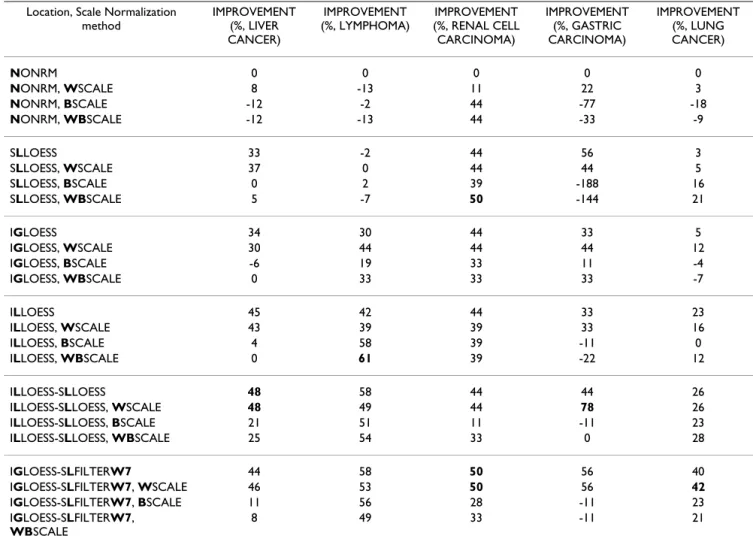
Table 8: IMPROVEMENT of the scale normalization methods. IMPROVEMENT is described in detail in Table 6. For a given data set, the biggest IMPROVEMENT(s) is shown in bold. The methods and data sets are described in Tables 3 and 4, respectively.
Location, Scale Normalization method IMPROVEMENT (%, LIVER CANCER) IMPROVEMENT (%, LYMPHOMA) IMPROVEMENT (%, RENAL CELL CARCINOMA) IMPROVEMENT (%, GASTRIC CARCINOMA) IMPROVEMENT (%, LUNG CANCER) NONRM 0 0 0 0 0 NONRM, WSCALE 8 -13 11 22 3 NONRM, BSCALE -12 -2 44 -77 -18 NONRM, WBSCALE -12 -13 44 -33 -9 SLLOESS 33 -2 44 56 3 SLLOESS, WSCALE 37 0 44 44 5 SLLOESS, BSCALE 0 2 39 -188 16 SLLOESS, WBSCALE 5 -7 50 -144 21 IGLOESS 34 30 44 33 5 IGLOESS, WSCALE 30 44 44 44 12 IGLOESS, BSCALE -6 19 33 11 -4 IGLOESS, WBSCALE 0 33 33 33 -7 ILLOESS 45 42 44 33 23 ILLOESS, WSCALE 43 39 39 33 16 ILLOESS, BSCALE 4 58 39 -11 0 ILLOESS, WBSCALE 0 61 39 -22 12 ILLOESS-SLLOESS 48 58 44 44 26
ILLOESS-SLLOESS, WSCALE 48 49 44 78 26
ILLOESS-SLLOESS, BSCALE 21 51 11 -11 23
ILLOESS-SLLOESS, WBSCALE 25 54 33 0 28
IGLOESS-SLFILTERW7 44 58 50 56 40
IGLOESS-SLFILTERW7, WSCALE 46 53 50 56 42
IGLOESS-SLFILTERW7, BSCALE 11 56 28 -11 23
IGLOESS-SLFILTERW7,
WBSCALE
Rank summary for scale normalization methods
Figure 7
Rank summary for scale normalization methods. The median ranks and upper quantile ranks are defined as described in Figure 5. The bar plots present a visual depiction of the results in the table. (Mean ranks are shown in pink; median ranks are shown in blue.) In each plot, normalization strategies are arranged in the following order: a location normalization method, a location normalization method followed by WSCALE (+WSCALE), a location normalization method followed by BSCALE (+BSCALE), a location normalization method followed by WBSCALE (+WBSCALE).
Location, Scale normalization method Median Rank Upper Quantile Rank
Nonorm 19.5 19.5 Nonorm,Wscale 17.5 22.5 Nonorm,Bscale 22 23.5 Nonorm,WBscale 23 23.5 sLloess 9 17.5 sLloess,Wscale 8 15.5 sLloess,Bscale 17 19.5 sLloess,WBscale 16 22 iGloess 9.5 15 iGloess,Wscale 10 11 iGloess,Bscale 18.5 21 iGloess,WBscale 18.5 19.5 iLloess 8 9.5 iLloess,Wscale 11.5 13 iLloess,Bscale 17 17.5 iLloess,WBscale 14.5 19.5 iLloess–sLloess 4.5 6
iLloess–sLloess,Wscale 4.5 8
iLloess–sLloess,Bscale 12 17.5
iLloess–sLloess,WBscale 11 14.5
iGloess–sLfilterW7 3 3
iGloess–sLfilterW7,Wscale 3 3.5
iGloess–sLfilterW7,Bscale 13 17.5
iGloess–sLfilterW7,WBscale 14.5 17.5
Nonorm +Wscale +Bscale
+WBscale 0 5 10 15 20 25
sLloess +Wscale +Bscale
+WBscale 0 5 10 15 20 25 iGloess +Wscale +Bscale +WBscale 0 5 10 15 20 25 iLloess +Wscale +Bscale +WBscale 0 5 10 15 20 25 iLloess Ŧ
sLloess +Wscale +Bscale
+WBscale 0 5 10 15 20 25 iGloess Ŧ
sLfilterW7 +Wscale +Bscale +WBscale
0 5 10 15 20 25
Due to the above two caveats, the relative rankings of the investigated normalization strategies can hardly be obtained accurately in this work. For example, our results show that IGLOESS-SLFILTERW7, ISTSPLINE-SLLOESS and IGLOESS-SLLOESS reduce LOOCV classification errors most consistently and effectively across all five data sets. It is difficult, however, to determine further which of these three strategies is the best, because small differences in classification results can either arise from inherent dif-ferences in these approaches and/or from the variability introduced by the LOOCV error estimator and less opti-mal k-NN classifiers. Moreover, our results should not be taken as a warrant of directly using baseline methods, such as k-NNs without feature selection, for high-dimen-sional classification tasks. More investigations are needed to understand the interplay between normalization (which improves data quality) and feature selection (which improves the classifier by throwing away non-informative data) to ascertain normalization strategies to produce an optimal classifier.
Conclusion
Using LOOCV error of k-NNs as the evaluation criterion, we assessed a variety of normalization methods that remove spatial effect, intensity effect and scale differences from cDNA microarray data. Overall, the single-bias-removal location approaches (which remove either spa-tial- or intensity effect from the data) perform better than GMEDIAN and NONRM, while the double-bias-removal location strategies (which remove both spatial- and inten-sity effect) perform better than the single-bias-removal location approaches. Of the 41 different strategies exam-ined, IGLOESS-SLFILTERW7, ISTSPLINE-SLLOESS and IGLOESS-SLBSCALE, all of which are two-step approaches and remove both intensity effect at the global level and spatial effect at the local level, appear to be the most effective at reducing LOOCV classification error. The investigated scale normalization methods do not have beneficial effect on classification performance. These results also indicate that spatial- and intensity effect do have profound impact on downstream data analyses, such as classification, and that removing these effects can improve the quality of such analyses.
Methods
Extant data sets and software
Table 4 summarizes relevant information on the cDNA microarray data sets from the Stanford Microarray Data-base (SMD) reexamined here. These data sets were selected because the published studies assayed samples from distinct cancers, the profiling experiments were per-formed at different times, four out of the five data sets were produced by different investigators, and the microar-rays used were printed with different probes on different
occasions. The LYMPHOMA study has been used as the illustrative, running example.
A variety of computational tools for manipulating, ana-lyzing, and visualizing microarray data are available. These include open source implementations based on the R language for statistical computing http://www.r-project.org[37] such as the Bioconductor http://www.bio conductor.org, MAANOVA http://www.jax.org/staff/ churchill/labsite/software/download.html, tRMA http:// www.pi.csiro.au/gena/tRMA, and braju http:// www.maths.lth.se/help/R/aroma packages. Standard R and Bioconductor packages and functions were used apart from one normalization method found in MAANOVA (joint removal of both spatial- and intensity effect at the global microarray level, IGSGBSCALE) and two normalization methods found in tRMA (removal of spatial effect at the local PT level, SLFILTERW3 and SLFILTERW7).
Pre-normalization data processing
For each spot, the foreground red (Rf) and green (Gf) quantitated fluorescent intensities (acquired using Gene-Pix image analysis software) of the arrayed DNA sequences were used to compute the non-normalized log ratio, M = log2(Rf / Gf), and average log intensity, . Because of the concern that local back-ground values estimated by GenePix may add additional noise to the data [3], these values were not subtracted from their corresponding foreground values. For a given microarray, the log ratios were normalized using location-and/or scale-normalization techniques and its particular configuration (the LYMPHOMA and GASTRIC CARCINOMA studies employed microarrays with two and three distinct configurations respectively).
Normalization methods
Tables 1 and 2 summarize the 23 location normalization methods that remove none, one, or both of spatial- and intensity effect (detailed descriptions of how they adjust
M values can be found elsewhere
[4,6,12,13,17,21,38,39]). In particular, Table 1 includes two methods that remove no spatial- or intensity-depend-ent dye bias: (i) NONRM neither removes any effect nor alters the distribution of M values; and (ii) GMEDIAN does not remove any effect but acts as a baseline normal-ization method because it sets the mean or median of M to zero. There are eight methods that remove either spatial- or intensity effect: (i) SLBSCALE removes spatial effect at the PT level using lowess; (ii) SLFILTERW3 and SLFILTERW7 remove spatial effect using median filters of the block sizes 3 × 3 and 7 × 7, respectively [17]; (iii) IGB -SCALE removes intensity effect at the global level; (iv) ILBSCALE removes intensity effect at the local level and as