Fast Clustering Using a Grid-Based Underlying Density Function Approximation

(1)

DigitalCommons@Kennesaw State University

Master of Science in Computer Science Theses Department of Computer Science

Spring 4-15-2020

Fast Clustering Using a Grid-Based Underlying Density Function

Approximation

Daniel Brown

Kennesaw State University

Follow this and additional works at: https://digitalcommons.kennesaw.edu/cs_etd

Part of the Other Computer Sciences Commons, and the Theory and Algorithms Commons

Recommended Citation Recommended Citation

Brown, Daniel, "Fast Clustering Using a Grid-Based Underlying Density Function Approximation" (2020). Master of Science in Computer Science Theses. 31.

https://digitalcommons.kennesaw.edu/cs_etd/31

This Thesis is brought to you for free and open access by the Department of Computer Science at

DigitalCommons@Kennesaw State University. It has been accepted for inclusion in Master of Science in Computer Science Theses by an authorized administrator of DigitalCommons@Kennesaw State University. For more

(2)

Fast Clustering Using a Grid-Based Underlying Density

Function Approximation

A Thesis Presented to

The Faculty of the Computer Science Department

by

Daniel Brown

In Partial Fulfillment

of Requirements for the Degree Master of Science, Computer Science

Kennesaw State University January 2020

(3)

Fast Clustering Using a Grid-Based Underlying Density

Function Approximation

Approved:

_______________________________ Dr. Yong Shi – Thesis Committee Chair _______________________________ Dr. Selena He – Committee Member _______________________________ Dr. Xiaohua Xu – Committee Member _______________________________ Dr. Coskun Cetinkaya - Department Chair _______________________________ Dr. Jon Preston - Dean

(4)

In presenting this thesis as a partial fulfillment of the requirements for an advanced degree from Kennesaw State University, I agree that the university library shall make it available for inspection and circulation in accordance with its regulations governing materials of this type. I agree that permission to copy from, or to publish, this thesis may be granted by the professor under whose direction it was written, or, in his absence, by the dean of the appropriate school when such copying or publication is solely for scholarly purposes and does not involve potential financial gain. It is understood that any copying from or publication of, this thesis which involves potential financial gain will not be allowed without written permission.

(5)

Notice To Borrowers

Unpublished theses deposited in the Library of Kennesaw State University must be used only in accordance with the stipulations prescribed by the author in the preceding statement.

The author of this thesis is:

Daniel Brown

1100 S Marietta PKWY, Marietta, GA 30060 The director of this thesis is:

Dr. Yong Shi 1100 S Marietta PKWY,

Marietta, GA 30060

Users of this thesis not regularly enrolled as students at Kennesaw State University are required to attest acceptance of the preceding stipulations by signing below. Libraries borrowing this thesis for the use of their patrons are required to see that each user records here the information requested.

(6)

Fast Clustering Using a Grid-Based Underlying Density

An Abstract of A Thesis Presented to

by

Daniel Brown

Bachelor of Science, Kennesaw State University, 2017

of Requirements for the Degree Master of Science, Computer Science

(7)

Abstract

Clustering is an unsupervised machine learning task that seeks to partition a set of data into smaller groupings, referred to as “clusters”, where items within the same cluster are somehow alike, while differing from those in other clusters. There are many different algorithms for clustering, but many of them are overly complex and scale poorly with larger data sets. In this paper, a new algorithm for clustering is proposed to solve some of these issues. Density-based clustering algorithms use a concept called the “underlying density function”, which is a conceptual higher-dimension function that describes the possible results from the continuous data set that our input data is just a discrete sample of. The algorithm proposed in this paper seeks to use this concept by creating a piecewise approximation of the underlying density function, and then merging points towards local density maxima from this higher-dimensioned space. First, the data space is divided into a grid-based structure and the density of each grid is calculated. Second, each of these “grid-squares” determines the densest space in its local area. Finally, the grid squares are merged together in the direction of their local density maximum, ultimately merging with one of the density maxima that form the root of a cluster. The experimental results show significant time improvements over standard algorithms such as DBSCAN with no accuracy penalty. Furthermore, the algorithm is also suitable for use with parallel and distributed systems, as an implementation with Apache Spark showed proper parallel scaling with low data set sizes required to overtake the serial implementation.

(8)

Fast Clustering Using a Grid-Based Underlying Density

A Thesis Presented to

by

Daniel Brown

of Requirements for the Degree

Master of Science, Computer Science

Advisor: Dr. Yong Shi

(9)

ACKNOWLEDGEMENTS

I would like to thank my Advisor, Dr. Yong Shi, for his expertise, guidance, support, and patience. Without his help I would never have gotten into the field of data analysis, let alone research it. I would also like to thank Arialdis Japa, another former student of Dr. Shi’s who I worked alongside for over a year. Finally, I would like to thank my family for their support, especially my fiancée for being with me every step of the way. Without her support I don’t think I would have been able to finish graduate school, let alone this thesis.

(10)

Experiments

...36

(11)

5.1.1 Data Sets ...36 5.1.2 Experimental Procedures ...38 5.1.3 Results ...39 5.2 Parallel Experiments ...44 5.2.1 Data Sets ...44 5.2.2 Experimental Procedures ...44 5.2.3 Results ...45 VI.

CONCLUSION

...49 VII.

REFERENCES

...52

(12)

LIST OF TABLES

Table 1. Synthetic Data Set Information ...37

Table 2. Real Data Set Information ...38

Table 3. Synthetic Data Runtime Averages ...40

Table 4. Real Data Runtime Averages ...40

Table 5. Synthetic Data Accuracy Comparison ...43

Table 6. Real Data Accuracy Comparison ...43

(13)

LIST OF FIGURES

Figure 1. Sample One-Dimensional Data Set ...16

Figure 2. Illustration of Grid Space Density Calculation ...17

Figure 3. Illustration of Densest Neighbor Determination ...17

Figure 4. Illustration of Cluster Creation ...18

Figure 5. Grid Space Density Calculation Pseudocode ...19

Figure 6. Densest Neighbor Determination Pseudocode ...22

Figure 7. Cluster Creation Pseudocode ...24

Figure 8. Parallel Data Import and Grid Square Assignment Pseudocode ...30

Figure 9. Parallel Grid Square Density Calculation Pseudocode ...30

Figure 10. Parallel Densest Neighbor Determination Pseudocode ...32

Figure 11. Parallel Cluster Creation Pseudocode ...34

Figure 12. Synthetic Data Runtime Difference vs Number of Instances ...41

Figure 13. Real Data Runtime Difference vs Number of Instances ...41

Figure 14. Parallel and Serial Runtime Comparison ...46

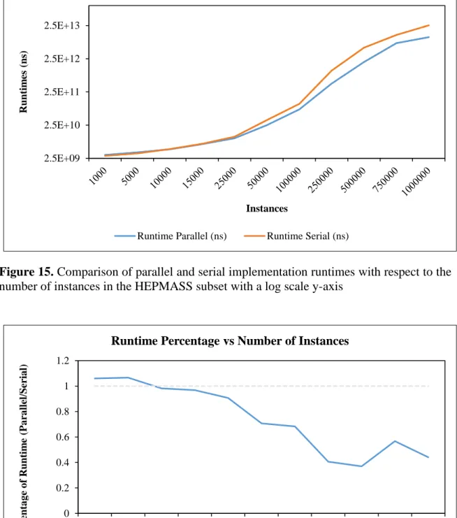
Figure 15. Log Scale Parallel and Serial Runtime Comparison ...48

(14)

CHAPTER I

INTRODUCTION

Clustering is an unsupervised machine learning task common in the world of data analysis. Clustering algorithms seek to discover groupings of related data within a dataset, each of which is referred to as a cluster. As clustering is an unsupervised task, it must do so without utilizing any external information or training datasets. Clustering’s ability to determine trends in data while only looking at the data itself has made it very attractive as an early-stage part of image recognition and many other data analysis tasks. Clustering algorithms exist in many different forms, which are broadly separated into classes of algorithms. The most common form of clustering are the Partitioning methods such as k-means which simply partition the set into clusters based on a metric such as Euclidian distance. There is also Density-based clustering which views the data points as individual instances of output from a higher-level underlying density function, and clusters are viewed as areas of relatively high density that correspond to areas that function is more likely to produce results. Grid-based methods seek to use a grid substructure to reduce the amount of calculations needed by scaling off of the number of grids instead of the number of records. Hierarchical methods seek to create a hierarchy of clusters, each at a different level of strictness, to show sub-clusters within normal clusters. Fuzzy clustering is also a commonly seen technique in which each record may exist in several clusters simultaneously, having a similarity measure for each instead of a binary yes or no to belonging.

(15)

All of these different types of algorithms result in a wide selection when it comes to choosing a clustering algorithm. Different algorithms are suitable for different applications, and as such, many different algorithms are useful for real-world data analysis. In this paper, we propose a new clustering algorithm that combines the underlying principles of density-based clustering methods with the grid structure from grid-based methods. By doing so we are able to maintain accuracy on par with other density-based methods while having the algorithm itself scale off of the grid substructure, resulting in greatly reduced runtimes. Throughout this paper, this algorithm will be referenced as the Density-Grid algorithm.

One of the most important elements of modern real-world data analysis, with or without involving clustering, are the concepts of parallel and distributed computing (known collectively as “High-Performance Computing” or HPC). Due to the massive sizes and complexities of modern “Big Data” datasets, running analysis algorithms in serial is unfeasible. As such, all real-world data analysis of importance utilizes HPC in order to vastly reduce runtimes. As such, this paper also discusses our attempts to parallelize the Density-Grid algorithm, in order to show its viability for real-world use, and we ultimately propose a parallel implementation using Apache Spark.

The rest of this paper is organized as follows. Chapter II discusses the related work and research, Chapter III discusses the Density-Grid algorithm and its development, Chapter IV discusses the parallel implementation of the Density-Grid algorithm, Chapter V covers our experiments and results for both the serial and parallel implementations, and Chapter VI summarizes our work with the Density-Grid algorithm and its contribution to the field.

(16)

CHAPTER II

RELATED WORK

This chapter is divided into two parts: Clustering Algorithms and Parallel

Computing Frameworks. Both subjects are important for the discussion of our work, so in this section we summarize previous work and research involving these two domains.

2.1 Clustering Algorithms

A wide range of traditional and novel clustering algorithms exist, and attempting to summarize each and every one is a task beyond the scope of this paper. As such, this section will focus on a selection of important traditional algorithm research and more modern novel algorithms, with an aim towards discussing the different classes of clustering and their strengths and weaknesses.

The clustering algorithm most familiar to many will be the venerated k-Means Clustering algorithm proposed by several authors but most concretely in [1] by Edward W. Forgy. This algorithm takes advantage of an iterative process in order to divide data points into clusters, focusing on their similarity to the centroids of clusters. The algorithm operates by first selecting k points in the data set to operate as the initial cluster centroids. Then the distance of each data point to each of the centroids is computed, with each point being assigned to the cluster whose centroid it they are closest to. The mean

(17)

of every point assigned to each cluster is then taken, with these mean values becoming the new values of the cluster centroids. These steps are repeated until the change in centroid values between iterations is below a certain threshold, at which point it is said to have converged. This algorithm is, as previously stated, one of the most well-known clustering algorithms and the first that many learn. It is not without its flaws however, given its nature as a first-of-its-kind algorithm. The first of these notable flaws is its run-to-run variance. In traditional k-means, the initial centroids are chosen randomly, and this random choice can lead to wildly different results at convergence. Second is the fact that k-means only accurately detects circular clusters, as traditionally Euclidian distance is used to determine distance, which causes a circular region around each cluster to be favored over any other shape. Finally, there is a trait many algorithms using traditional distance measurements share, which is poor accuracy scaling in high-dimensioned space due to the “Curse of Dimensionality” spreading points out. Much research exists modifying the k-means algorithm to address these shortcomings, and it is widely viewed as the most important of the “partitioning” class of clustering methods.

Next, we focus on the Density-based class of clustering algorithms, most notably represented by the DBSCAN algorithm in [2] by M. Ester, H. P. Kriegel, J. Sander, and X. Xu. Density-based algorithms in general see data as instances of output that, taken together, produce a continual higher-dimension underlying density function, and see clusters as areas of space that are relatively dense with points, with those regions being where the underlying density function is most likely to produce output. DBSCAN visits each point in a data set, looking at an area surrounding this point to determine whether it has a local density great enough to justify assuming it to be part of a cluster. This is

(18)

controlled via two parameters: ε, how large of a neighborhood to search, and minPts, how many data points are required to be found in a neighborhood to count as a cluster. Each point is visited in an arbitrary order, the number of points in its ε-neighborhood is observed, and it is then decided whether this point and its ε-neighborhood constitute a new cluster or whether the point itself should be considered noise until further notice. If noise, then the point will be unclustered unless it is later added to a cluster from being in another point’s ε-neighborhood. Otherwise, if the number of points passes the minPts

threshold, the point and all of the points in its ε-neighborhood are added to a cluster, and any points in those points’ ε-neighborhoods are also added to the cluster. This algorithm is well regarded and heavily used to this day, with only a few shortcomings. The main weakness being that having a single static value for ε means that DBSCAN can have issues detecting meaningful clusters if the density of data between clusters vary greatly. Much research has been devoted to modifying DBSCAN to improve performance for various cases of data, but the core algorithm is still considered the standard for clustering algorithms.

One such modification to DBSCAN is the OPTICS algorithm proposed in [3] by M. Ankerst, M. Bruenig, H. P. Kriegel, and J. Sander. The OPTICS algorithm is very similar to DBSCAN, but seeks to address the varying density issue by also calculating a core distance, defined as the distance from a point to the minPtsth point closest to it. Having both this core distance and ε allows OPTICS to consider different densities of clusters. This improvement has made it very attractive for use in many applications, however the additional processing slows it down compared to DBSCAN, with the authors of OPTICS

(19)

showing its runtimes to consistently be approximately 1.6 times slower than those of DBSCAN.

Another form of clustering is hierarchical clustering, in which a hierarchy of clusters and subclusters are represented in a manner similar to a tree graph, allowing for the relations between these varying levels of relation in clusters to be viewed in a logical form. The most well-known algorithm for hierarchical clustering is BIRCH, proposed in [4] by T. Zhand, R. Ramakrishnan, and M. Livny. BIRCH was originally created to modify hierarchical clustering for large data sets by doing a large amount of preprocessing that is not reliant on having the global data structure in memory. BIRCH constructs a tree of clustering features by reducing a set of data points into three values: the number of points, the linear sum of the points, and the square sum of the points. These features are each set as a node in a tree, and then a more traditional agglomerative hierarchical algorithm is used to do the clustering on the CF nodes. This allows for efficient clustering based only on the relevant information. Hierarchical clustering results in an overview of all of the different clusters present and their relations; however, the process does result in long runtimes since multiple levels/rounds of clustering must occur.

In [5], W. Wang, J. Yang, and R. Muntz proposed the STING algorithm for grid-based clustering. In STING, the data space is recursively divided into a grid structure, with the initial data space having 4 grid subsections, each of which has 4 grid subsections, which repeats until it reaches a set number of layers. The clustering and processing is then done on these subsections instead, allowing the algorithm to scale based on the number of grids instead of on the number of data points. Splitting the data into separate

(20)

units also allows algorithms such as STING to be efficiently parallelized, as they overcome the issue of data dependency (discussed in section 2.2). The reliance on grid substructures can result in a loss of accuracy however, as points are considered as a group and not individually.

In [6], R. Agrawel, J. Gehrke, D. Gunopuloa, and P. Raghaven propose CLIQUE, a subspace clustering algorithm which seeks to determine clusters that exist not just in the set of all dimensions, but in any given subset of the data’s dimensions as well. It first separates each dimension into a set of independent grids based on a gridSize parameter. The number of points in each grid of each dimension is compared to a threshold parameter that determines if it counts as a “dense” grid or not. Each combination of dimensions is then investigated, with the overlaps of dense grids from each dimension in the subset being flagged as dense subspaces that are likely to contain clusters. This approach allows for effective cluster detection without as extensive dimension reduction or feature selection preprocessing as many other algorithms, but becomes very reliant on the gridSize and threshold parameters being suitable for the data set involved. This algorithm also scales well compared to the number of data points, but is much more sensitive to the dimensionality of the data, as it must look at each subset of dimensions. The final traditional method to be discussed is the Fuzzy c-means clustering algorithm proposed in [7] by J. C. Dunn. This algorithm takes advantage of fuzzy set theory, in which any individual point may actually belong to more than one set or cluster. In fuzzy c-means this is represented by the use of a membership coefficient. In other terms, in a normal partitioning clustering method, a point has the value 0 or 1 for belonging to a given cluster, while in fuzzy c-means it instead has a value from 0 to 1,

(21)

representing its degree of similarity to that cluster. Fuzzy c-means determines these values in a process much like that of k-means discussed previously. It begins by randomly assigning membership coefficients from each cluster to each point. Then it iteratively determines the centroid of each cluster based on these coefficients, and then updates the coefficients based on this new cluster centroid. This process is repeated until the coefficients converge and become stable. This algorithm suffers from many of the same problems as k-means with regards to the random initial values, but the use of the fuzzy logic properties allows for unique information compared to many other clustering methods.

The first recent novel algorithm to be discussed is dGridSlink, proposed in [8] by Goyal et al. This algorithm is an extension of GridSlink, which itself is an extension of SLINK, or “single linkage”, which is a hierarchical clustering algorithm. GridSlink seeks to use a grid structure to allow the SLINK algorithm better scaling while still maintaining a good approximation of results. The distributed form of GridSlink is dGridSlink. This algorithm demonstrates two important concepts that will be built upon later: Parallel/Distributed computing is vital for efficient data analysis work, and grid-based algorithms are prime candidates for parallelization due to their reduced data dependency between calculations in the same stage.

In [9], D. Huang et al propose U-SPEC, which is a hybrid spectral clustering method. Spectral clustering methods utilize the concept of eigenvalues to cluster in a reduced dimension set in order to avoid issues with the “curse of dimensionality.” Hybrid methods are an increasingly common type of clustering that uses multiple classes of clustering methods together to create a new approach. U-SPEC uses a combination of a

(22)

representative data point selection method to select a subset of data points, and an approximation method to then reduce this set into K representatives. Spectral clustering is then performed on this reduced subset.

In [10], D. Huang, C. Wang, and J. Lai propose an ensemble clustering method based on local weights and uncertainty estimation. Ensemble clustering methods typically seek to create multiple clusterings of the data set, before analyzing them and creating a final clustering based on the most common similarities between the base clusterings. This work seeks to use a system of more flexible local weight and uncertainty measures as opposed to the more common global weights. This allows for variation in the distribution and uncertainty of individual clusters. They also propose novel consensus functions based on this difference.

In [11], R. Bhagawati, S. R. Lasker, and B. Swain proposed an algorithm for clustering with quantum computers, combining the knowledge of classical clustering algorithms with quantum physics. They do this by using quantum mechanics to represent each piece of data as a vector, and then using the Schrödinger Equation to perform a clustering on these vectors. This work demonstrates that clustering is an important task, even within new fields such as Quantum Computing, and that new classes of clustering algorithms are actively being developed.

2.2 Parallel Computing Frameworks

Parallel Computing, frequently discussed in combination with Distributed Computing and referred to as High Performance Computing (HPC), is a computing concept that has become vastly important in the modern field of data analysis. It is the

(23)

process of breaking a larger calculation or task down into a number of smaller components, each of which may be independently processed by different computing units. This allows multiple operations to be done in parallel, increasing the speed of computation. As modern data sets have dramatically increased in size, this technology has become vital to data analysis tasks. There are many ways to take advantage of parallel computing, but the most common ones are a pair of frameworks that allow for easy development of parallel algorithms while allowing all of the low-level implementation details to be handled by said frameworks. The two frameworks most commonly used are MapReduce and Apache Spark.

MapReduce was proposed in [12] by J. Dean and S. Ghemawat, two computer scientists working at Google. It was created to be a simple-to-use framework for implementing parallel computations and allowing them to be efficiently done on very large distributed data sets. The main structure of MapReduce revolves around two operations: map and reduce. A map operation is a function that maps each piece of data in the data set to a key-value pair. The reduce operation is a function that takes all of the value pairs with the same key and aggregates them in order to create a final key-value pair, with a single entry per unique key. This framework was revolutionary as it allowed for a user-friendly programming interface that allowed users to focus primarily on the logical operations, without worrying about the lower-level communications work. MapReduce quickly gained traction in the data analysis world, and became the de facto standard for parallel data analysis work. It was not without criticism however, as many pointed out its shortcomings. These include it being limited to solely map and reduce operations and not being able to implement any others, which some claim limit the tasks

(24)

it may be applied to, and its inability to store temporary files in the computing clusters’ main memory in favor of hard disks, which greatly slows down communication.

Spark was originally proposed in [13] by M. Zaharia, M. Chowdhury, M. J. Franklin, S. Shenker, and I. Stoica; researchers at the University of California, Berkeley’s AMPLab. It was later donated in its entirety to the Apache Software Foundation, who currently maintain the project. It was created in order to address some of the aforementioned shortcomings with MapReduce. Spark’s key building block is the concept of a Resilient Distributed Dataset, or RDD. An RDD is a dataset that is distributed in an error-resistant way across all of the worker nodes, and the flow of a Spark program is based on a series of Transformations and Actions being performed on these RDDs. The wide range of available transformations allow for Apache Spark to be much more flexible than MapReduce, overcoming the restrictive single Map into single Reduce program structure of MapReduce. In [14] the Apache Software Foundation covers the majority of the available transformations and actions in the current version of Apache Spark (ver. 2.4.5). Transformations take an RDD and transform the data within into some new form, also to be stored in an RDD while Actions simply perform an action on the data in an RDD with the results being returned in a non-distributed form to the driver node. Map still exists as a transformation; however, there are a wide range of forms from a simple 1-to-1 map or mapByKey, to a 1-to-many flatMap, to the many-to-1 mapPartitions. Reduce exists as well, with reduce itself being an action while reduceByKey exists as a transformation for Key-Value pair RDDs. Other transformations like count, countByKey, repartition, aggregateByKey, union, intersection, and takeSample allow Spark applications to be very flexible. Spark also

(25)

allows control of data storage locations, allowing for datasets to be processed in main memory, greatly increasing the speed of processing.

Both MapReduce and Apache Spark have been widely used with data processing algorithms, including clustering. In [15], Y. He et al used MapReduce to create a parallel implementation of the DBSCAN algorithm, showing runtime improvements over that of the traditional serial implementation. In [16], G. Luo, X. Luo, T. F. Gooch, L. Tian, and K. Qin similarly implemented DBSCAN with Apache Spark, also showing runtime improvement, illustrating that both frameworks are suitable for use with parallel data analysis. Many other authors have also contributed to the body of work for MapReduce and Apache Spark data analysis algorithm implementations. Following is a selection of recent or important papers detailing relevant work.

In [17], Y. Xu, W. Qu, Z. Li, G. Min, K. Li, and Z. Liu implement a version of the

k-means algorithm known as k-means++ with MapReduce. The k-means++ algorithm uses a sequential process to select cluster centroids in a non-random manner. This process is not guaranteed to result in an optimal centroid choice, but it is shown that it is very close to the optimal solution and much more accurate than the traditional method. Their paper discusses the challenges involved with parallelizing the k-means++ algorithm, as it traditionally scales poorly with dataset size. They do this by using the k -means++ initialization algorithm to combine two MapReduce stages from the traditional

k-means MapReduce implementation, allowing for a runtime reduction with a close approximation to the optimal k-means results. This paper highlights that fact that with MapReduce you must code in a linear fashion, with a single MapReduce job consisting of a single map stage followed by a single reduce stage (there is technically a shuffle

(26)

operation between the two, but that is automated and handled by the framework). This means that in order to parallelize some algorithms with MapReduce, tricks must be done to reduce the number of repeated stages.

In [18], W. Huang, L. Meng, D. Zhang, and W. Zhang showcase the ability of Apache Spark to perform its operations in-memory. They introduce a generic model for parallel processing of remote sensing data, and, using a massive dataset of remote sensing data, they demonstrate the performance gains inherent in using Spark to process the data in-memory. This is important as it demonstrates how Spark’s capabilities were influenced by the shortcomings of MapReduce. It is true that MapReduce is still widely popular, but features such as in-memory processing have allowed Apache Spark to challenge it for its crown as the go-to parallel processing framework.

In [19], B. Liu, S. He, D. He, Y. Zhang and M. Guizani demonstrate a parallel implementation of the Fuzzy c-means algorithm using Apache Spark. Their implementation was specialized for Agricultural Image data, but the work is applicable to data analysis using fuzzy c-means in other fields. The results predictably show a significant increase in performance compared to the traditional serial implementation. The significance of this paper comes from the fact that is a recent paper (being published in 2019) showing how research into the real-world applications of Apache Spark is currently an area of great interest. Currently much research is being done to optimize and implement algorithms for Apache Spark, and to show how these improvements make the tasks viable for use in real-world data analysis tasks.

In [20], J. Franklin, S. Wenke, S. Quasem, L. A. Carraher, and P. A. Wilsey propose streamingRPHash, a MapReduce-based parallel clustering algorithm that seeks to

(27)

cluster only a random projection of the data. This is done in order to improve scaling with large datasets, as many traditional clustering methods do not scale well with data set size. Furthermore, the authors discuss how this random sampling may actually serve to increase security and anonymity of data. This paper illustrates how parallel algorithms alone may not be enough to improve data scaling enough for real world use, as well as showing the advantages of not scaling directly off of data point, even in a parallel/distributed environment.

(28)

CHAPTER III

Density-Grid Clustering Algorithm

The Density-Grid algorithm was originally designed in order to address many of the factors important to clustering discussed in the previous sections. Our main goal was to improve runtimes for large data sets, specifically focusing on the algorithm’s scaling with regards to data set size and suitability for parallelization. In addition, we wanted for the algorithm to be able to detect clusters of arbitrary shape, to not have the number of clusters as an input value, and to attempt to reduce the impact of high-dimensionality on accuracy. We decided on a combination of ideas from the Density-based and Grid-based classes of clustering algorithms. By utilizing a grid structure, we sought to scale at least part of our calculations not on the number of data points, but on the number of grids, thereby reducing complexity. By using the concepts of density-based clustering methods, we sought to handle arbitrary shapes of clusters and to have relatively high accuracy.

We achieved these goals by focusing on a core idea of the Density-based class of algorithms: the Underlying Density Function. The idea of the underlying density function is that the data in our data set is just a series of individual observations, with the set of all possible observations being the product of some higher-dimensioned function. The concept follows that the areas of higher density in our data set represent the areas that the underlying density function is maximized, or where more results are likely to be located in the continual spectrum. In order to merge this idea with the

(29)

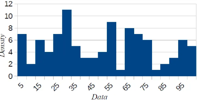
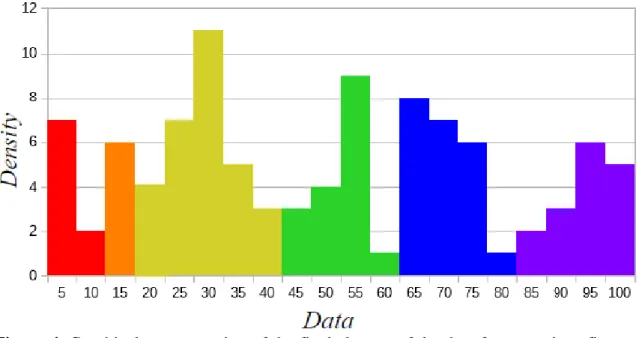
concepts from grid-based clustering, we used a grid structure to create a piecewise approximation of this underlying density function, and then merged the grid cells towards their local density maxima, having them fall towards local maximums in the underlying density function. This piecewise approximation is very similar in form to that of the rectangle rule for approximation the value of an integral. Much as in the rectangle rule, we collapse a continuous function value inside of a “bin” into a singular representative value. This value is then used as an approximation for the higher dimensioned result. This process is illustrated with figures 1 and 2. These figures show, using a sample one-dimensional dataset, how we use the density of the grid squares to add an additional dimension and create the piecewise approximation of the continuous underlying density function. Figures 3 and 4 then show how each grid square is either the densest in its area, or has a denser one as a neighbor that it is assigned to, and how these assignments result in a final clustering.

The concepts explained above allowed us to use the high-level concept of the underlying density function to create what is ultimately an algorithm with a simplicity, and resultant speed, that belies its true nature. The algorithm consists of three phases, each of which will be discussed in more algorithmic detail in the following subsections; however, figures 2 through 4 also serve as a visual representation of the process, each corresponding to the output of a phase.

Figure 1. Graphical representation of a sample one-dimensional data set, displayed on a number line.

(30)

Figure 2. Graphical representation of the density “binning” of the data set from Figure 1

with a grid size of 5. The number of data points in each grid were totaled, resulting in a value for that grid square’s density. Arranging these densities as a second dimension along the original data shows how these density values resemble the rectangle rule, and work as a piecewise approximation of the underlying density function. This process of determining grid square location and grid square density comprises phase one of the algorithm.

Figure 3. Graphical representation of the relationship between neighboring grid squares from figure 2. Squares with a vertical bar are the local density maxima that form the cores of the clusters, while all other grid squares have an arrow pointing to the left or the right, depending on which neighbor has the highest density. The determination of core status or densest neighbor location comprises phase two of the algorithm.

(31)

Figure 4. Graphical representation of the final clusters of the data from previous figures. Each chain of densest neighbor assignments has been collapsed and all squares merged with one of the core squares to form a final cluster that surrounds a local maximum of the underlying density function. This process of using the densest neighbor information to form the final clusters comprises phase three of the algorithm.

3.1 Grid Square Density Calculation

Phase one of the Density-Grid Clustering Algorithm is the Grid Square Density Calculation phase. In this phase we iterate through the data set and assign each point to a grid square, while maintaining a density measurement for each of the grid squares. The pseudocode for this phase of the algorithm is shown in Figure 5.

The input for this phase of the algorithm is two items: our list of data points in the form of a List data structure containing arrays of doubles (each dimension of each data point being a double in the array) and our only runtime variable, a double

(32)

Figure 5. Pseudocode representation of the first phase of the Density-Grid Clustering Algorithm. This phase consists of assigning each data point to a grid square and determining the density of each grid square

We begin by initializing a new list that we use to build our output, utilizing a custom class called GridSquare. This class represents a grid square, and contains the GridSquare’s identification array, a list of points, and a density measurement, in addition to several useful methods. We then iterate over each data point, first determining which GridSquare a given data point belongs to. GridSquares are

(33)

grid in each dimension. To calculate which GridSquare the data point we are looking at belongs to, we use the following equation on each dimension of the data point:

(𝑖𝑛𝑡) ⌊ 𝑑[𝑖] 𝑔𝑟𝑖𝑑𝑆𝑖𝑧𝑒⌋

We divide each dimension by the gridSize value and then floor the result, as that is how the GridSquares’s identifications works. This number is then cast to an integer to serve as the identification array of a GridSquare. Now that we have a GridSquare id array, we search our list of GridSquares to see if this GridSquare object has been created yet. If it has, then we add this point to that GridSquare object’s list of points and increment its density value by one. If it has not been created, we create it, add this data point, and then add the new GridSquare to the above list.

The final output of this phase is a List of GridSquares, each containing a set of points and a density measure corresponding to the number of points contained in that GridSquare. This output List is then utilized by the following phase to determine the densest neighbor of each GridSquare.

3.2 Densest Neighbor Determination

Phase two of the algorithm is the Densest Neighbor Determination phase. In this phase we determine the densest neighboring grid square for each grid square, or if it is denser that all of its neighbors. For this algorithm we define a neighboring grid square as one where the identification array of the two does not differ by more than one space in any dimension. By not relying on a traditional distance metric, we theorize that this

(34)

may also be somewhat effective at countering the curse of dimensionality. The pseudocode for this algorithm is shown in Figure 6.

The input for this phase is the list of GridSquare objects created during the previous phase. We will return the same list at the end, however, each GridSquare in the list will have been updated with a pointer to the GridSquare that is its densest neighbor (or itself, if it is its own densest neighbor and therefore the core of a cluster).

We begin by creating a new list of GridSquares that is the same as the original list but sorted by descending density. This means that the first object in this new temporary List is the densest GridSquare that exists. We do this in order to reduce the complexity of comparisons for the following steps, as well as to maintain clustering accuracy of any set of neighboring grid squares with equal-and-highest density.

Once we have our temporary list, we begin iterating over all of the GridSquares in the original list. We then use a nested for loop to compare this GridSquare to each of the GridSquares in the sorted list. This ensures we are comparing in order of highest-to-lowest density. By sorting the list beforehand, we ensure that the first neighbor we find will either be the densest neighbor or tied for densest. Being tied only matters if there are several neighboring grid squares of equal density which are also all local density maxima. In that case, the first one in the list will be chosen as the core square, preventing errors. Since the first neighbor we find is guaranteed to be the densest one, all we have to do is check them in order. We must also ensure that the density of a given GridSquare is not less than the one for which we wish to determine the densest neighbor. If so, it means that that square is its own densest neighbor.

(35)

Figure 6. Pseudocode representation of the second phase of the Density-Grid Clustering Algorithm. This phase consists of determining the densest neighbor of each GridSquare.

The GridSquare class has a field for a pointer to another GridSquare, which we use to point to each GridSquare’s densest neighbor once it is found. If it is determined that a GridSquare is its own densest neighbor, then a pointer to itself is added instead. Once the iteration over the initial List is complete, we have the same list but with each GridSquare object having that pointer field filled. We then return that List so that it can get used for the third phase.

(36)

3.3 Cluster Creation

Phase three of the algorithm is Cluster Creation, in which we determine our final clusters. The input for this phase is the List of GridSquares with their densestNeighbor field filled in from the previous phase. The output of this phase is a List of Cluster objects, which are from a custom Cluster class that contains a List of GridSquares belonging to that cluster as well as several helper methods. The pseudocode for this phase is shown in Figure 7.

We begin by initializing a new list of cluster objects that we will use to build our clustering piece-by-piece. We then start the main iterative part of the phase by iterating over every gridSquare in the input list and then check to see if that gridSquare and its DensestNeighbor are included in a cluster yet. This may occur due to a point having been the densest neighbor of a previous point, or due to two points sharing a densest neighbor. The custom findCluster method we use to check returns -1 if the gridSquare does not belong to a cluster yet, or, if it does belong to a cluster, an integer value corresponding to that cluster’s position in the global list.

We then have a flow of logic that determines what step we take in order to cluster both the gridSquare and its densestNeighbor. We first check to see if a cluster is its own densest neighbor, which determines if it is a core or not. If it is a core, we check to see if it has already been included in a cluster due to being another point’s

densestNeighbor. If it has, then we are done with this GridSquare. If it has not been clustered, then we create a new cluster object and add this gridSquare.

(37)

Figure 7. Pseudocode representation of the third phase of the Density-Grid Clustering Algorithm. This phase consists of determining the final clustering.

(38)

If a gridSquare is not a core square, then we have to check if either it or its

densestNeighbor are clustered yet. If neither of the two gridSquares has been clustered yet, then we create a new Cluster object and add both gridSquares to it. If either one, but not both, of the gridSquares are in a cluster, then we add the other gridSquare to that cluster as well. If both belong to different clusters, then we must merge those two clusters together.

After this logic is applied to each gridSquare in the global list, we are guaranteed to have a final list of clusters that contains every gridSquare (and therefore every point) between them. This is our final clustering.

(39)

CHAPTER IV

Parallel Implementation Using Apache Spark

In order to parallelize the Density-Grid algorithm, several challenges need to be overcome. In general, the largest challenge when parallelizing algorithms is the concept of “data dependency”. Since different pieces of data are being processed on different nodes of the cluster, if calculations are dependent on other calculations or data that is not on the same node, communication between nodes must occur for the calculation to proceed. In our case, the three-phase design of the algorithm was

originally conceived in order to address this issue. Within each phase of the algorithm, every calculation is independent of other calculations in that phase. Global information is produced at the end of phases one and two that is needed in the phases after them, but this can be done using communication tools built into Spark. Ultimately this means that the design of the parallel implementation is very similar to that of the serial, with the three phases separated by communications, and the logic placed within Spark transformations so as to operate in parallel.

Spark’s systems of RDDs, actions, and transformations was mentioned previously, but in order to describe the work done in the parallel implementation, the

transformations and actions used need to be described in more detail. Specifically, the functions to be discussed are: map, mapToPair, countByKey, collect, broadcast, and parallelize.

(40)

First are map and mapToPair, the main tools used in the implementation. We mainly use mapToPair, but as it is a specialized form of map, both must be discussed. As discussed previously, Spark uses a data structure called a Resilient Distributed Dataset, or RDD, as its basis. Data is stored and distributed across the cluster in these structures, with each node having part of the data. The map transformation is the most basic form of transformation in Spark. The notation of the transformation is that it transforms the RDD from one form of data to another, mapping the input to the output. This is accomplished by using the map transformation to denote a function to be applied to each item in the source RDD. This function must take as input the data type or types of a single record from the source RDD, and returns a new record of the same or a different data type. In this manner you are able to apply a function to all of the data points in an RDD in a distributed manner. MapToPair is the same as map, but it is used to map an RDD to a key-value pair RDD instead of a single-value one. In a single-value RDD, each record is a single variable and they are all the same type. In a key-value pair RDD, each record consists of two variables and the key and value can be different types. The keys are non-unique, as they are frequently used to denote a relationship or belonging to a group.

Our second spark feature to discuss, countByKey, can only be used on a key-value pair RDD, and utilize the non-uniqueness of the key. countByKey is an action, not a transformation, as it does not result in a new RDD. CountByKey is a distributed way to count how many records have the same key, and return this information back to the driver node as a “Map” data structure (not to be confused with the map Spark transformation) relating each unique key to the number of records with that key.

(41)

The third feature is collect, which is also an action. Collect takes an RDD and has all of the information stored in it across all of the nodes, and sends it all to the driver node as a list. Its name is appropriate, as it collects all of the data to a single node. This can be useful if serial processing is needed, or if communications work needs to be done like in the case of information needed globally.

The fourth feature is how Spark allows for global information to be sent. Normally only RDDs are stored across each node, and all other data structures created are stored locally on the driver node. Broadcast, however, allows us to send a variable from the driver node to every worker node, so that that variable is available for use within transformations.

Finally, we have the parallelize action. Parallelize is used to create a new RDD from some list local to the driver node. In this sense it is collect, but in reverse. There are many ways to create RDDs, including a built-in-function to read and parallelize a text file without the user having to do any processing, but parallelize is the most versatile of these methods as it can turn any List object into as RDD.

Now that we have discussed the main transformations and actions we will be using; we can look at the implementation in more detail. As before, the algorithm is split into three phases, and each will be discussed in its own subsection.

4.1 Grid Square Density Calculation

This phase corresponds to the phase discussed in 3.1. In this phase we seek to take our data, assign each point to a grid square, and then find the total density of each grid square. The input for the parallel form of this phase is a text file containing our data in

(42)

CSV format (each line is a record, and individual dimensions are separated by commas), and a double value corresponding to our grid size. The output will be an RDD of gridSquares and a global list of gridSquare densities. The pseudocode for this phase is shown in Figures 8 and 9. Figure 8 details the Grid Space determination while Figure 9 details the density calculations and communications work.

First, we must turn our text file data into an RDD. Apache Spark has a built-in method for this, which is just Spark.textFile(). This automatically reads in the text file and distributes it out to the worker nodes as an RDD of strings. In order to work with the data, we need it in the form of doubles, not strings (specifically as arrays of

doubles). Luckily, we can transform the data from strings to double arrays in the same mapToPair operation we use to determine which grid square it belongs to.

The main work of this first part of the phase is done in a single mapToPair

transformation. In this transformation, the work done is very similar to that done in the first phase of the original algorithm. The mapToPair consists of code to retrieve our data point as a double array from the initial string, and then the original logic used to determine which grid square a point belongs to based on its offset from the origin in each dimension. In order to retrieve a double array, we split the string at each comma, and then parse each individual substring into a double. The equation for determining the gridSquare is the same as discussed in section 3.1. We divide the data point by gridSize and then floor the result. We then return each record in the form of a key-value pair, with a gridSquare object as the key and our data point as the key-value.

(43)

Figure 8. Pseudocode representation of the parallel implementation of the first half of Phase 1 of the algorithm.

Figure 9. Pseudocode representation of the parallel implementation of the second half of Phase 1 of the algorithm.

(44)

We now take our intermediate RDD and use the second feature of Spark we discussed earlier: countByKey. Since our key values correspond to the grid squares, countByKey will, in parallel, count how many data points belong to each grid square and return this information to the driver node in the form of a Map data structure. This is the information we will need in the next phase, but we need it in a slightly different form. We first convert the Map structure to a simple List of gridSquares, with their densities stored inside of the gridSquare object. We then sort this list of gridSquares by decreasing density, much as in the serial form of the algorithm. Now that we have the data in the form we want it, we need to send that data to each worker node, so that it is globally available. To do this we use the broadcast feature of Spark to transfer the data, and then retrieve it in each node as the List. Finally, we parallelize our List as well, creating a new RDD. By doing this, we now have an RDD consisting only of a single record per grid square, instead of multiple records per grid square. This new RDD and the global density list are the output from this phase used in phase 2.

4.2 Densest Neighbor Determination

This phase corresponds to the phase discussed in 3.2. In this phase we seek to identify what each grid square’s densest neighboring grid square is, or if it is its own densest neighbor and therefore the core of a cluster. The input for the parallel form of this phase is a global list of GridSquares and their densities, sorted in order of

decreasing density, and an RDD of gridSquares. The output will be a global Map data structure connecting each data point to its densest neighbor. The pseudocode for this phase is shown in figure 10.

(45)

Figure 10. Pseudocode representation of the parallel implementation of phase 2 of the algorithm.

We begin with a mapToPair transformation containing all of the algorithmic work. In this mapToPair, we follow the same procedure from the serial algorithm, where we compare our current gridSquare to each gridSquare in the sorted list, stopping when we

(46)

find a neighbor or a gridSquare with a density lower than the current gridSquare’s. The resulting key-value pair in the new RDD always has the key of our current gridSquare, and the value is either our densest neighbor, if one exists, or this point again if it is its own densest neighbor.

Now that we have an RDD relating each grid square to its densest neighbor, we want to retrieve it to the driver node so that we can broadcast it and make it a global variable, so that it can be used by the worker nodes in phase 3. To do this, we use a special form of collect called collectAsMap. CollectAsMap does the same thing as collect, but instead of returning the RDD as a local list of tuples, it returns it as a Map data structure with the same key-value pair relations as our RDD. We collect it as a Map for quick and efficient look up in phase 3. We then use the same system of broadcast and value retrieval as in phase 1 to ensure that we have this Map of densest neighbors available as a global variable.

4.3 Cluster Creation

This phase corresponds to the phase discussed in 3.3. In this phase we seek to utilize the densest neighbor information from phase 2 to create our final clusters. The input for the parallel form of this phase is a global map of gridSquares and their densest neighbors, and the same RDD of gridSquares used in phase 2. The output will be a local list data structure corresponding to our final clusters. This list will have the form of a List of tuples, where the first value in each tuple is the core gridSquare, and the second value is a List of grid squares in the cluster with that core. The pseudocode for this phase is shown in figure 11.

(47)

Figure 11. Pseudocode representation of the parallel implementation of phase 3 of the algorithm.

This is the first parallel phase where the function done within our main mapToPair takes on a significantly different form than that of the serial form of this phase. Since the serial version constructs our clusters piece-by-piece using global information, we

(48)

are not able to use the exact same procedure here. Instead we use the concept that each cluster has a core grid square, and seek to determine which core square each grid square belongs to. We can then use this notation to construct our final clusters. In order to determine the core cluster each grid square belongs to; we have to follow the chains of densest neighbors until we find a grid square that is its own densest neighbor. We do this by, for each grid square in the RDD, looking it up in our map to find its densest neighbor. If it is not already a core grid square because of its densest neighbor being itself, we continue following the chain of densest neighbors, looking up each new neighbor in the map until we find that core grid square. We then return a new record as a key-value pair where the key is the core grid square and the value is our current grid square. This results in an RDD with one record per grid square, with those squares as the values and the final grid square that is their root as the keys.

Since, outside of some very extreme corner case data sets, there are fewer clusters, and therefore core squares, than grid squares overall, this means that the keys are non-unique. This is important as we are then able to use the groupByKey transformation to reduce our RDD down to a single record per cluster. GroupByKey first shuffles the partitioning of an RDD so that each record with the same key is on a single node. It then combines the values of those records into a List structure, and sets that as the value field of a new key-value pair. In this manner we go from our RDD of one record per grid square to an RDD with one record per cluster, with a key of the core square of the cluster and the value of a list of all of the grid squares belonging to that cluster. We are then able to collect this to the driver node as a List, with each record in the list corresponding to a single cluster.

(49)

CHAPTER V

Experiments

This section describes the procedures and results from the experiments used to test the algorithm in both serial and parallel. The serial experiments will be discussed in section 5.1, while the parallel experiments will be discussed in section 5.2.

5.1 Serial Experiments

5.1.1 Data Sets

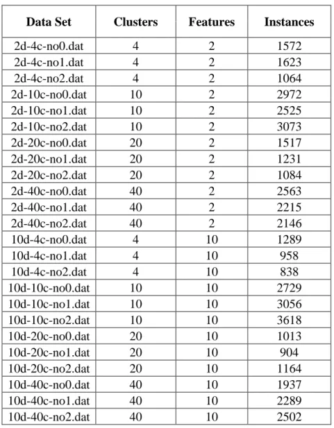
Two types of data sets were used for the serial experiments: synthetically generated data sets created by Julia Handl from the University of Manchester [21] detailed in Table 1, and ten well-known real data sets from the UCI Machine Learning Repository [22] – [31] detailed in Table 2. The synthetic data sets are relatively low-noise

compared to the real data sets, which is why a selection of both were used.

Julia Handl is an associate professor at the University of Manchester who created a cluster generator that could create high-dimensional data sets with ground-truth

clusters to be used as test data for clustering algorithms [21]. The website hosting the information and source code for her generators also contains 160 sample data sets produced by the generator, of which 24 were selected for use in this testing. Table 1 details the relevant information about each selected data set.

(50)

Table 1. Synthetic data set information for serial experiments

Data Set Clusters Features Instances

2d-4c-no0.dat 4 2 1572 2d-4c-no1.dat 4 2 1623 2d-4c-no2.dat 4 2 1064 2d-10c-no0.dat 10 2 2972 2d-10c-no1.dat 10 2 2525 2d-10c-no2.dat 10 2 3073 2d-20c-no0.dat 20 2 1517 2d-20c-no1.dat 20 2 1231 2d-20c-no2.dat 20 2 1084 2d-40c-no0.dat 40 2 2563 2d-40c-no1.dat 40 2 2215 2d-40c-no2.dat 40 2 2146 10d-4c-no0.dat 4 10 1289 10d-4c-no1.dat 4 10 958 10d-4c-no2.dat 4 10 838 10d-10c-no0.dat 10 10 2729 10d-10c-no1.dat 10 10 3056 10d-10c-no2.dat 10 10 3618 10d-20c-no0.dat 20 10 1013 10d-20c-no1.dat 20 10 904 10d-20c-no2.dat 20 10 1164 10d-40c-no0.dat 40 10 1937 10d-40c-no1.dat 40 10 2289 10d-40c-no2.dat 40 10 2502

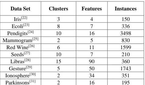
The real data sets were all retrieved from the UCI Machine Learning Repository, and represent a wide range of different fields and types of observations [22] – [31]. Many of the data sets selected are well known and frequently used for testing data analysis algorithms. There is a wide range of dimensionality, amount of data points, and number of clusters. Table 2 details the relevant information about each of these data sets.

(51)

Table 2. Real data set information for serial experiments

Data Set Clusters Features Instances

Iris[22] 3 4 150 Ecoli[23] 8 7 336 Pendigits[24] 10 16 3498 Mammogram[25] 2 5 830 Red Wine[26] ₆ ₁₁ ₁₅₉₉ Seeds[27] 10 7 210 Libras[28] 15 90 360 Gesture[29] 5 50 1743 Ionosphere[30] ₂ ₃₄ ₃₅₁ Parkinsons[31] 2 16 195

5.1.2 Experimental Procedures

Each data set was processed using both the Density-Grid clustering algorithm and the DBSCAN algorithm. They were run 10 times through each algorithm to calculate an average runtime, as both algorithms are guaranteed to result in the same final clustering accuracy (in comparison to an algorithm like k-means that has a random initialization). An optimal-to-the-thousandsth input variable was used for each algorithm to ensure fairness. Final clustering accuracy was calculated using the Adjusted Rand Index, a commonly-used metric for cluster similarity. The Rand Index works by, for every pair of data points in the data set, comparing the experimental and labeled clusterings to see whether those two data points are in the same or different clusters in each clustering. This means it serves as a measure of how often the two clusterings agree or disagree. The Adjusted Rand Index corrects for chance, giving a more accurate result.

DBSCAN was used for comparison for several reasons. It is one of the most, if not the most, widely used clustering algorithms in existence, and is well-regarded for both

(52)

its accuracy and runtimes. Furthermore, it is also a density-based clustering algorithm like our Density-Grid algorithm, meaning the two are very similar in terms of capabilities and are therefore suitable for comparison. Both handle arbitrary shapes of clusters, have a single input variable, and utilize similar underlying concepts in regards to the representation of clusters as dense areas of space.

Our tests were run on a university-provided computing cluster with 24 computing threads, Apache Hadoop as management software, and YARN as our resource allocator, with the code for both algorithms being implemented using Java.

5.1.3 Results

The two main metrics by which a clustering algorithm can be judged are its runtimes and accuracy. We will start with runtimes, as that is the metric we are most heavily targeting with our algorithm design.

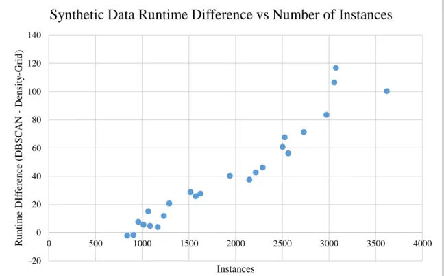
Table 3 summarizes the results of the synthetic data runtime testing, showing and average runtime difference of 40.77ms, which is 49 percent faster on average. More importantly, the difference in runtime between the two algorithms increases with regards to the number of data points in each data set as shown in Figure 12.

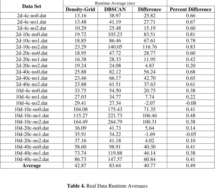
In Table 4 we look at the results from the real data tests, which have a similar improvement with an average runtime difference of 38.05ms, or 51 percent. Like the synthetic tests, we also see a trend of the runtime difference increasing with respect to the number of data points, as shown in Figure 13.

(53)

Table 3. Synthetic Data Runtime Averages

Data Set Runtime Average (ms)

Density-Grid DBSCAN Difference Percent Difference

2d-4c-no0.dat 13.16 38.97 25.82 0.66 2d-4c-no1.dat 13.48 41.19 27.71 0.67 2d-4c-no2.dat 10.29 25.48 15.19 0.60 2d-10c-no0.dat 19.72 103.23 83.51 0.81 2d-10c-no1.dat 18.85 86.46 67.61 0.78 2d-10c-no2.dat 23.29 140.05 116.76 0.83 2d-20c-no0.dat 18.95 47.72 28.77 0.60 2d-20c-no1.dat 16.38 28.33 11.95 0.42 2d-20c-no2.dat 19.24 24.08 4.83 0.20 2d-40c-no0.dat 25.88 82.12 56.24 0.68 2d-40c-no1.dat 23.46 66.17 42.70 0.65 2d-40c-no2.dat 23.88 61.51 37.63 0.61 10d-4c-no0.dat 33.75 54.50 20.75 0.38 10d-4c-no1.dat 27.03 34.77 7.74 0.22 10d-4c-no2.dat 29.41 27.34 -2.07 -0.08 10d-10c-no0.dat 104.08 175.43 71.35 0.41 10d-10c-no1.dat 115.27 221.73 106.46 0.48 10d-10c-no2.dat 164.49 264.79 100.31 0.38 10d-20c-no0.dat 36.09 41.73 5.64 0.14 10d-20c-no1.dat 35.91 34.22 -1.69 -0.05 10d-20c-no2.dat 37.16 41.18 4.02 0.10 10d-40c-no0.dat 58.60 98.91 40.30 0.41 10d-40c-no1.dat 73.74 119.88 46.14 0.38 10d-40c-no2.dat 86.73 147.57 60.84 0.41 Average 42.87 83.64 40.77 0.49

Table 4. Real Data Runtime Averages

Data Set Runtime Average (ms)

Density-Grid DBSCAN Difference Percent Difference

Iris 5.60 5.52 -0.08 -0.01

Ecoli 7.92 8.81 0.89 0.10

Pendigits 127.93 352.97 225.04 0.64

Mammogram 11.42 26.74 15.32 0.57

Red Wine Quality 42.36 70.28 27.93 0.40

Seeds 8.68 10.65 1.97 0.18 Libras 31.09 36.37 5.28 0.15 Gesture 90.76 195.07 104.32 0.53 Ionosphere 22.92 22.10 -0.82 -0.04 Parkinsons 9.81 10.44 0.63 0.06 Average 35.85 73.90 38.05 0.51

(54)

Figure 12. Synthetic data runtime with respect to the number of instances in the data set

Figure 13. Real data runtime with respect to the number of instances in the data set -20 0 20 40 60 80 100 120 140 0 500 1000 1500 2000 2500 3000 3500 4000 R u n tim e DI ff er en ce ( DB SC A N -Den sity -Gr id ) Instances

Synthetic Data Runtime Difference vs Number of Instances

-50 0 50 100 150 200 250 0 500 1000 1500 2000 2500 3000 3500 4000 R u n tim e DI ff er en ce ( DB SC A N -Den sity -Gr id ) Instances

(55)

Next, we look at accuracy with Table 5 detailing the results of our synthetic testing. We see the two algorithms being relatively similar in terms of accuracy, with one or the other usually being slightly more or less accurate than the other. There are occasional outliers with one being much more accurate than the other, but the final average Adjusted Rand Index accuracy difference of only 0.01% proves the closeness of accuracy.

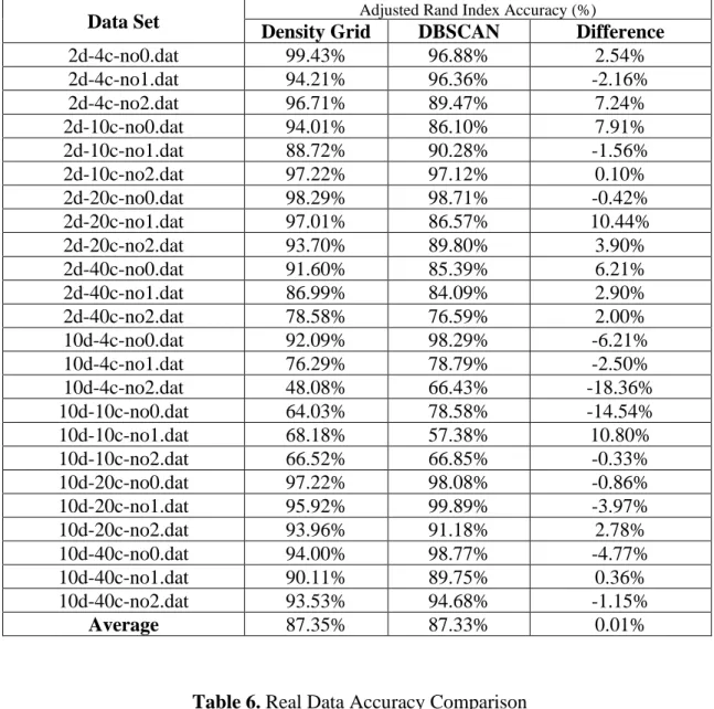
Table 6 shows the real data testing for accuracy, and shows more variance. A few data sets are very closely matched, but in many cases the specific nature of one of the data sets causes one or the other of the algorithms to be a significantly better fit. Interestingly enough, the Adjusted Rand Index accuracy difference measure ends up being 10.01% higher for our algorithm, but this is likely due to the difference in noise handling between the two algorithms. DBSCAN is very aggressive with noise handling, frequently refusing to place points it considers too noisy into a cluster. In a situation where each point has a ground-truth cluster label, this results in an artificial decrease in its Adjusted Rand Index score. This is why we only see this phenomenon in the relatively noisier real data sets. By comparison, our algorithm makes a best-faith attempt to cluster each data point, as the piecewise approximation nature makes it ill-suited for determining if individual points are too noisy or not, instead clustering them as an entire grid square.

(56)

Table 5. Synthetic Data Accuracy Comparison

Data Set Adjusted Rand Index Accuracy (%)

Density Grid DBSCAN Difference

2d-4c-no0.dat 99.43% 96.88% 2.54% 2d-4c-no1.dat 94.21% 96.36% -2.16% 2d-4c-no2.dat 96.71% 89.47% 7.24% 2d-10c-no0.dat 94.01% 86.10% 7.91% 2d-10c-no1.dat 88.72% 90.28% -1.56% 2d-10c-no2.dat 97.22% 97.12% 0.10% 2d-20c-no0.dat 98.29% 98.71% -0.42% 2d-20c-no1.dat 97.01% 86.57% 10.44% 2d-20c-no2.dat 93.70% 89.80% 3.90% 2d-40c-no0.dat 91.60% 85.39% 6.21% 2d-40c-no1.dat 86.99% 84.09% 2.90% 2d-40c-no2.dat 78.58% 76.59% 2.00% 10d-4c-no0.dat 92.09% 98.29% -6.21% 10d-4c-no1.dat 76.29% 78.79% -2.50% 10d-4c-no2.dat 48.08% 66.43% -18.36% 10d-10c-no0.dat 64.03% 78.58% -14.54% 10d-10c-no1.dat 68.18% 57.38% 10.80% 10d-10c-no2.dat 66.52% 66.85% -0.33% 10d-20c-no0.dat 97.22% 98.08% -0.86% 10d-20c-no1.dat 95.92% 99.89% -3.97% 10d-20c-no2.dat 93.96% 91.18% 2.78% 10d-40c-no0.dat 94.00% 98.77% -4.77% 10d-40c-no1.dat 90.11% 89.75% 0.36% 10d-40c-no2.dat 93.53% 94.68% -1.15% Average 87.35% 87.33% 0.01%

Table 6. Real Data Accuracy Comparison

Data Set Adjusted Rand Index Accuracy (%)

Density Grid DBSCAN Difference

Iris 79.87% 79.87% 0.00%

Ecoli 74.03% 50.04% 23.99%

Pendigits 50.23% 62.35% -12.12% Mammogram 34.52% 18.46% 16.06% Red Wine Quality 9.32% 4.22% 5.11%

Seeds 70.88% 40.93% 29.95% Libras 21.40% 24.57% -3.17% Gesture 19.07% 24.05% -4.98% Ionosphere 35.17% 21.96% 13.21% Parkinsons 38.67% 6.65% 32.02% Average 43.32% 33.31% 10.01%

(57)

5.2 Parallel Experiments

5.2.1 Data Sets

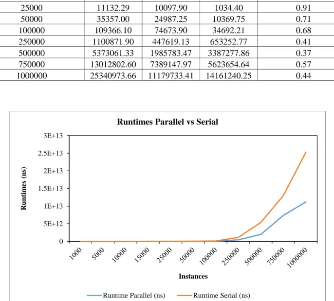
The parallel experiments were conducted using the HEPMASS data set from the UCI Machine Learning Repository [32]. The HEPMASS data set is data from a series of particle collision experiments, and features both testing and training data sets for both constant and variable particle masses. We are using a subset of the constant mass training set, which consists of 7000000 instances with 27 features each. We tested 11 subsets, ranging from 1000 to 1000000 instances, as that was the top end of what our computing cluster could handle.

5.2.2 Experimental Procedures

We ran each subset of the HEPMASS data set through both our serial implementation and our parallel implementation of the Density-Grid clustering method, recording an average runtime