Evaluation of statistical methods, modeling, and multiple testing in RNA-seq studies

(1)

Theses & Dissertations Boston University Theses & Dissertations

2016

Evaluation of statistical methods,

modeling, and multiple testing in

RNA-seq studies

https://hdl.handle.net/2144/17727 Boston University

(2)

Dissertation

EVALUATION OF STATISTICAL METHODS, MODELING, AND

MULTIPLE TESTING IN RNA-SEQ STUDIES by

SEUNG HOAN CHOI

B.S., The State University of New York at Stony brook, 2008 M.A., Boston University, 2011

Submitted in partial fulfillment of the

requirements for the degree of

Doctor of Philosophy

(3)

SEUNG HOAN CHOI

(4)

First Reader ___________________________________________________ Anita L Destefano, Ph.D.

Professor of Biostatistics

Second Reader ___________________________________________________

Josée Dupuis, Ph.D.

Professor of Biostatistics

Third Reader ___________________________________________________

Kathryn L Lunetta, Ph.D.

(5)

To my beloved late grandfather

(6)

ACKNOWLEDGMENTS

I would like to thank all my committee members for all their support toward this degree. My sincerest gratitude goes to my primary advisor, Dr. Anita L

Destefano, for her all guidance and support throughout my time at Boston

University. She always helped me think toward the right direction, obtain insights to see the whole picture, and concentrate on details where many may miss. This dissertation could not be finished without her expertise in statistical genetics and genomics and her insights.

I am very grateful to Dr. Josée Dupuis and Dr. Kathryn L Lunetta who shared their statistical expertise and supported my research. I would also like to thank Dr. Honghuang Lin and Dr. Richard H Myers for sharing ideas and offering advice and comments on my dissertation.

I also like to thank Dr. Sudha Seshadri, with whom I begin my research, for her support and guidance. Her enthusiasm toward research always motivates myself. With her support, I was enabled to participate in multiple large consortia and learn how to collaborate with other people.

I would like to thank my parents Geun Sik Choi and Hye Sook Kim and my sister Jina Choi for their unconditional love and support. Lastly, I would like to thank my

(7)

wife Kyung Hee Baek, to whom I dedicate my dissertation, for her love, support, and encouragement.

(8)

EVALUATION OF STATISTICAL METHODS, MODELING, AND MULTIPLE TESTING IN RNA-SEQ STUDIES

SEUNG HOAN CHOI

Boston University Graduate School of Arts and Sciences, 2016 Major Professor: Anita L Destefano, Professor of Biostatistics

ABSTRACT

Recent Next Generation Sequencing methods provide a count of RNA molecules in the form of short reads, yielding discrete, often highly non-normally distributed gene expression measurements. Due to this feature of RNA

sequencing (RNA-Seq) data, appropriate statistical inference methods are required. Although Negative Binomial (NB) regression has been generally accepted in the analysis of RNA-Seq data, its appropriateness in the application to genetic studies has not been exhaustively evaluated. Additionally, adjusting for covariates that have an unknown relationship with expression of a gene has not been extensively evaluated in RNA-Seq studies using the NB framework. Finally, the dependent structures in RNA-Seq data may violate the assumptions of some multiple testing correction methods. In this dissertation, we suggest an alternative regression method, evaluate the effect of covariates, and compare various

multiple testing correction methods. We conduct simulation studies and apply these methods to a real data set. First, we suggest Firth’s logistic regression for detecting differentially expressed genes in RNA-Seq data. We also recommend the data adaptive method that estimates a recalibrated distribution of test

(9)

statistics. Firth’ logistic regression exhibits an appropriately controlled Type-I error rate using the data adaptive method and shows comparable power to NB regression in simulation studies. Next, we evaluate the effect of disease-

associated covariates where the relationship between the covariate and gene expression is unknown. Although the power of NB and Firth’s logistic regression is decreased as disease-associated covariates are added in a model, Type-I error rates are well controlled in Firth’ logistic regression if the relationship between a covariate and disease is not strong. Finally, we compare multiple testing correction methods that control family-wise error rates and impose false discovery rates. The evaluation reveals that an understanding of study designs, RNA-Seq data, and the consequences of applying specific regression and multiple testing correction methods are very important factors to control family- wise error rates or false discovery rates. We believe our statistical investigations will enrich gene expression studies and influence related statistical methods.

(10)

TABLE OF CONTENTS

ACKNOWLEDGMENTS ... v

ABSTRACT ... vii

TABLE OF CONTENTS ... ix

LIST OF TABLES ... xiii

LIST OF FIGURES ... xvii

LIST OF ABBREVIATIONS ... xix

Chapter 1 Introduction ... 1

1.1 Gene expression studies ... 1

1.2 Negative Binomial regression ... 3

1.3 Logistic regression ... 5

1.4 Covariate Analysis ... 7

1.5 Multiple testing corrections ... 9

1.6 Dissertation outline ... 10

Chapter 2 Evaluation of Logistic Regression Models for Case-Control Study in RNA-Seq Analysis ... 13

2.1 Introduction ... 13

2.2 Dispersion estimation methods in negative binomial framework ... 15

(11)

2.3.2 Classical logistic regression ... 17

2.3.3 Bayes logistic regression ... 17

2.3.4 Firth’s logistic regression ... 18

2.4 Data Adaptive (DA) distribution of test statistics ... 18

2.5 Simulation study ... 19

2.5.1 Generation of simulated RNA-Seq data ... 20

2.5.2 Analysis of simulated RNA-Seq data ... 21

2.5.3 Cross-Validation of data adaptive method in simulated RNA-Seq data ... 22

2.6 Simulation result ... 23

2.6.1 Simulation Type-I error result ... 23

2.6.2 DA Type-I error simulation results ... 26

2.6.3 Empirical power simulation results ... 28

2.7 Application to RNA-Seq data of Huntington’s Disease (HD) ... 34

2.8 Permutation design ... 35

2.8.1 Generation of permuted RNA-Seq data ... 36

2.8.2 Analysis of permuted HD RNA-Seq data ... 36

2.9 Permutation result ... 38

2.9.1 Permutation Type-I error result ... 38

2.9.2 Permutation DA method Type-I error result ... 43

2.9.3 HD RNA-Seq data analysis results ... 46

2.10 Discussion ... 51

Chapter 3 Evaluation of Effect of Covariates for Case-Control Study in RNA- Seq Analysis ... 56

(12)

3.2 Analysis methods for evaluating effect of covariates ... 57

3.3 Simulation study ... 58

3.3.1 Generation of simulated RNA-Seq data ... 59

3.3.2 Generation of simulated covariate data ... 59

3.3.3 Analysis of simulated RNA-Seq data with simulated covariates ... 60

3.3.4 Cross-validation of data adaptive method in simulated RNA-Seq data ... 60

3.4 Simulation result ... 61

3.4.1 Type-I error simulation result ... 61

3.4.2 Type-I error simulation result with DA method ... 67

3.4.3 Empirical power simulation result ... 68

3.5 Application to the real RNA-Seq data set of Huntington’s Disease (HD) .. ... 72

3.5.1 Analysis of HD RNA-Seq data with simulated covariates ... 72

3.5.2 Result of HD RNA-Seq data with simulated covariates ... 73

Chapter 4 Multiple testing correction methods in RNA-sequence data ... 78

4.2 Methods ... 83

4.2.1 Multiple testing correction procedures controlling FWER ... 83

4.2.2 Multiple testing correction procedures controlling FDR ... 84

4.2.3 Simulation study ... 87

(13)

4.3.1 False positive rates from multiple testing correction procedures controlling

the FWER from simulated data ... 93

4.3.2 FDRs from multiple testing correction procedures controlling FDR using simulated data. ... 100

4.3.3 Power comparison among the multiple testing correction methods controlling FWER based on simulated data. ... 106

4.3.4 Power comparison among the multiple testing correction methods controlling FDR based on simulated data. ... 110

Chapter 5 Summary and future work ... 118

5.1 Summary ... 118

BIBLIOGRAPHY ... 120

CURRICULUM VITAE ... 127

(14)

LIST OF TABLES

Table 2.1 Parameters and their values in simulation scenarios ... 20 Table 2.2 Type-I error rates of the NB regressions with the true dispersion and

ML and QL dispersions from the balanced design ... 24 Table 2.3 Type-I error rates of the NB and logistic regressions from the balanced

design ... 25 Table 2.4 Type-I error rates of the NB and logistic regressions with the DA

method from the balanced design ... 27 Table 2.5 Empirical power of NB regression with the true dispersion and ML and

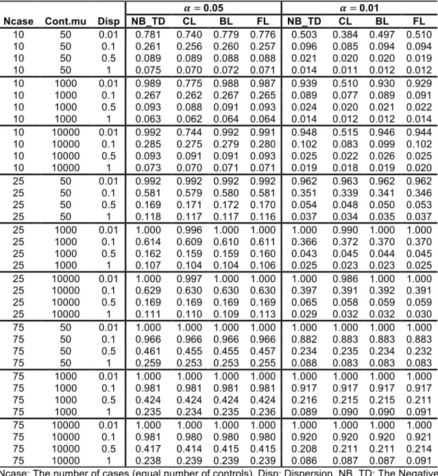
QL Dispersions from the balanced design with l2fc of 0.3 ... 29 Table 2.6 Empirical power of NB and logistic regressions from the balanced

design with l2fc equal to 0.03 ... 30 Table 2.7 Empirical power of NB and logistic regressions from the balanced

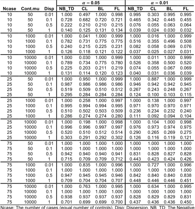
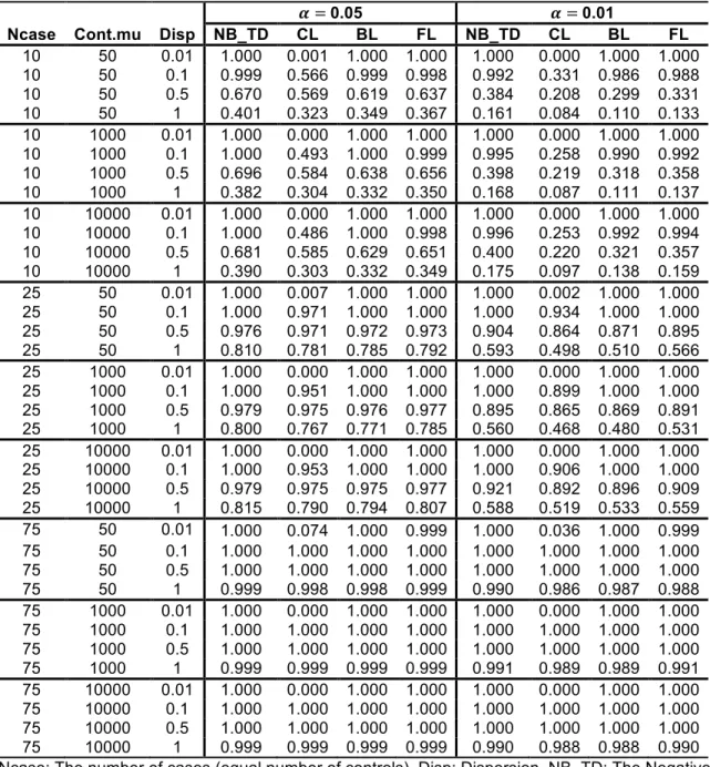
design with l2fc equal to 0.06 ... 31 Table 2.8 Empirical power of the NB and logistic regressions from the balanced

design with l2fc equal to 1.2 ... 32 Table 2.9 Empirical power of NB and logistic regressions from the balanced

design with l2fc equal to 2 ... 33 Table 2.10 Type-I error rates from DESeq2 analysis of permuted HD data with

mean expression value > 3 ... 41 Table 2.11 Type-I error rates from CL, BL, FL regressions of permuted HD data

(15)

Table 2.12 Type-I error rates from DESeq2 analysis with the DA method from the permuted HD data ... 44 Table 2.13 Type-I error rates from logistic models with the DA method from the

permuted HD data ... 46 Table 2.14 Top 10 genes from FL regressions among genes having FDR > 0.05

in DESeq2 and FDR < 0.05 in CL, BL, and FL regressions using the DA method ... 50 Table 2.15 Top genes from DESeq2 among genes having FDR > 0.05 in CL, BL

and FL regressions using the DA method ... 50 Table 3.1 Parameters and their values in simulation scenarios ... 58 Table 3.2 Type-I error rates of the NB regressions with the true dispersion and

ML and QL dispersions from balanced design of 10 cases and 1000 mean expressions ... 63 Table 3.3 Type-I error rates of the NB and Firth’s logistic regressions from

balanced design of 10 cases and 1000 mean expressions ... 64 Table 3.4 Type-I error rates of the NB and Firth’s logistic regressions from

balanced design of 25 cases and 1000 mean expression values ... 65 Table 3.5 Type-I error rates of the NB and Firth’s logistic regressions from

balanced design of 75 cases and 1000 mean expression values ... 66 Table 3.6 Type-I error rates of the NB and Firth’s logistic regressions with DA

(16)

Table 3.7 Summary of genomic inflation factor from HD analyses with simulated covariates ... 73 Table 4.1 Simulation parameters and values ... 91 Table 4.2 False positive rates for five cases and five controls from simulated data with no-correlation among differentially expressed genes based on analysis with edgeR. ... 98 Table 4.3 False positive rates for five cases and five controls from simulated data based on analysis with edgeR. ... 99 Table 4.4 False discovery rates for five cases and five controls from simulated

data with no-correlation among differentially expressed genes based on analysis with edgeR ... 104 Table 4.5 False discovery rates for five cases and five controls from simulated

data based on analysis with edgeR ... 105 Table 4.6 Power for sample size of five cases and five controls with no-

correlation among the differentially expressed genes based on analysis using edgeR and the multiple testing correction methods controlling FWER ... 108 Table 4.7 Power for the sample size of five cases and five controls based on

analysis using edgeR results and the multiple testing correction methods controlling FWER ... 109

(17)

Table 4.8 Power for the sample size of five cases and five controls in no-

correlation in differentially expressed genes based on analysis using edgeR and the multiple testing correction methods controlling FDR ... 113 Table 4.9 Power for the sample size of five cases and five controls based on

analysis using edgeR and the multiple testing correction methods controlling FDR ... 114

(18)

LIST OF FIGURES

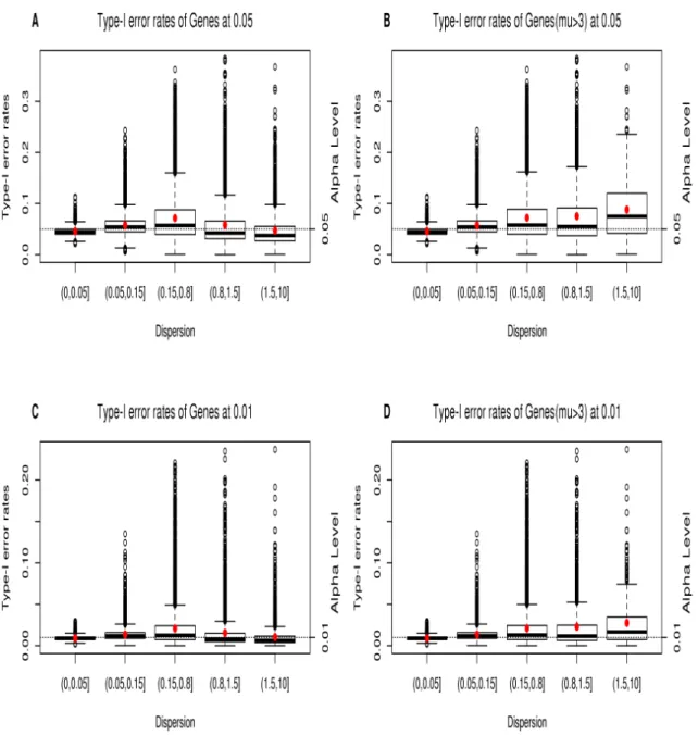
Figure 2.1 Type-I error rates from DESeq2 analysis of the permuted HD data .. 40

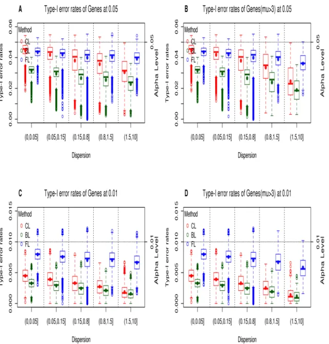
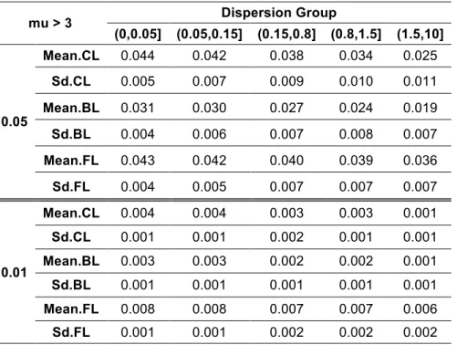
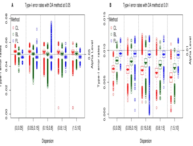
Figure 2.2 Type-I error rates from logistic models of the permuted HD data ... 42

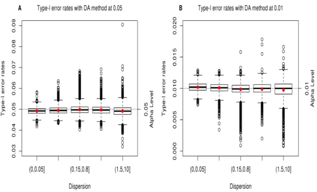
Figure 2.3 Type-I error rates from DESeq2 analysis with the DA method from the permuted HD data ... 44

Figure 2.4 Type-I error rates from logistic models with the DA method from the permuted HD data ... 45

Figure 2.5 Q-Q plots of HD data analysis by regression methods ... 48

Figure 2.6 Venn diagram of HD analysis results using DA method ... 49

Figure 3.1 Empirical power of NB and FL regressions with covariates for a balanced design with 10 cases and mean expression in controls of 1000 .. 69

Figure.3.2 Empirical power of NB and FL regressions with covariates for a balanced design with 25 cases and mean expression in controls of 1000 .. 70

Figure 3.3 Empirical power of NB and FL regressions with covariates for a balanced design with 75 cases and mean expression in controls of 1000 .. 71

Figure 4.1 False positive rates with 100% null hypotheses ... 95

Figure 4.4 False discovery rates with 95% null hypotheses ... 102

Figure 4.5 False discovery rates with 75% null hypotheses ... 103

Figure 4.6 Power with proportion of null hypotheses equal to 75% using the multiple testing correction methods controlling FWER ... 107

(19)

Figure 4.7 Power with proportion of null hypotheses equal to 95% using FDR methods ... 111 Figure 4.8 Power with proportion of null hypotheses equal to 75% using FDR

(20)

LIST OF ABBREVIATIONS

DE... Differential Expression FDR ... False Discovery Rate FWER ... Familywise Error Rate NB... Negative Binomial NCP ... Non Confounding Predictive NGS ... Next Generation Sequencing RNA ... Ribonucleic Acid RNA-Seq ... RNA sequencing

(21)

Chapter 1 Introduction 1.1 Gene expression studies

Gene expression studies have played important roles to understand phenotypic variation including how tissues vary in gene expression and how these variations are related to biologic function(Ramsköld et al. 2009). Current next generation sequencing (NGS) genome-wide gene expression measurement methods simultaneously quantify tens of thousands of unique Ribonucleic Acid (RNA) molecules extracted from biological samples. These RNA sequencing (RNA-Seq) methods produce data that can be transformed into numerical values that are proportional to the abundance of RNA molecules of interest, including protein-coding, processed transcript, pseudo-genes, miRNAs, tRNAs, rRNAs, snRNAs, snoRNAs, and scRNAs(Tarazona et al. 2011), and represent the amount of expression of those molecules. A common task in the analysis of RNA-Seq data is to evaluate the statistical differences of the mean expression of genes between sets of samples from two different conditions, e.g. control versus diseased patients. Identifying differentially expressed genes is the first important step to understanding the molecular mechanism of the differentially expressed genes and developing novel therapies for related diseases.

Microarray technology has been widely used to measure gene expression in the past decades. Microarray technology quantifies the fluorescence of specific RNA molecules and, after processing and normalization, expression values are

(22)

continuous and typically approximated by a normal distribution. Due to these characteristics of microarray data, well-understood methods like two sample t- tests and linear regression are often utilized to identify the association between expression level and disease status. In contrast, NGS methods provide a count of RNA molecules in the form of short reads, which are discrete measurements that do not follow a normal distribution. Consequently, statistical methods that assume normality are inappropriate for the analysis of these count data, and therefore the development of appropriate statistical methods is necessary.

Because the total number of reads of each sample will likely be different, a normalization step is required before analyzing the association between genes and a condition. Anders et al. proposed a normalization method that divides each count by the geometric mean count of the corresponding gene and takes the medians of these scaled counts within each library(Anders and Huber 2010). Robinson et al. developed the Trimmed Mean of M Values (TMM) method that computes each normalization factor from the trimmed mean of the gene-wise log fold-changes of the current library to a reference library(M. D. Robinson and Oshlack 2010). Mortazavi et al. suggested the standard reads per kilobase of transcript per million mapped reads (Mortazavi et al. 2008). An inappropriate normalization method may result in a biased differential expression (DE) inference(Bullard et al. 2010). Dillies et al. comprehensively evaluated

(23)

similar and reasonable results in their evaluating metrics(Dillies et al. 2013). Appropriately normalized data allow us to perform unbiased differential expression inferences.

1.2 Negative Binomial regression

Poisson models are a popular approach to analyze count data observed from experiments or epidemics. Poisson models assume that the data follow a Poisson distribution, where the mean and variance are the same. When the variance is significantly larger than the mean, alternative models are required to analyze the over-dispersed count data. A common alternative approach is the Negative Binomial (NB) model, also known as the gamma-Poisson model.

This approach fits a NB generalized linear model (McCullagh and Nelder 1989) to the data with estimated or fixed value of a dispersion parameter. Let Y be the response variable and 𝑥 be an explanatory variable. The marginal distribution of Y, and negative binomial likelihood are

𝑌~ NB 𝜇(𝑥), 𝜙 , 𝑤ℎ𝑒𝑟𝑒 𝜇 ≥ 0 𝑎𝑛𝑑 𝜙 ≥ 0 such that Pr 𝑌 = 𝑦|𝑥 = _{@ C}@(ABC_DE _@(ABF)DE) _FBC_DEF_G(H) C DE CDEG(H) FBCDE_{G H} A , 𝑦 = 0, 1, 2 … , E 𝑌|𝑥 = 𝜇, 𝑎𝑛𝑑 VAR 𝑌|𝑥 = 𝜇 + 𝜇Q_{𝜙 .}

When 𝜙 is close to zero, the distribution of Y becomes a Poisson distribution. Let 𝑌_S~ NB 𝜇(𝑥_S), 𝜙 , 𝑖 = 1, … , 𝑛 be independent, where 𝜇 𝑥_S = exp 𝑥_S𝛽 and 𝑥_S is the 𝑝×1 explanatory vector. The likelihood function is proportional to

(24)

𝐿 𝛽, 𝜙 = @ A\BCDE @ CDE _{@ A} \BF F FBCDE_{G H} \ CDE CDEG H\ FBCDE_{G H} \ A\ ] S^F ,

and the log 𝐿 𝛽, 𝜙 is

𝑙 𝛽, 𝜙 = A\dFlog 1 + 𝜙𝑗 +

e^f 𝑦Slog 𝜇 𝑥S − 𝑦S − 𝜙dF log (1 + 𝜙𝜇 𝑥S ]

S^F .

The obtained (𝛽_hi, 𝜙_hi) maximize 𝑙 𝛽, 𝜙 through scores and information iterations(McCullagh and Nelder 1989). However, in general, a variance parameter from maximum likelihood estimators is underestimated (M. D. Robinson and Smyth 2007), hence alternative methods are suggested for the estimation of 𝜙.

The pseudo-likelihood model (Breslow 1984) estimates the variance parameter using a distribution free goodness-of-fit statistic by solving the moment function

A\dGjk,\ l

G\(FBCmkDEGjk,\)= 𝑛 − 1

]

S^F .

The quasi-likelihood model (J. A. Nelder 2000) uses a deviance statistic rather than the Pearson statistic in the pseudo-likelihood model to estimate dispersion using a function

2 𝑦_Slog A\

Gjk,\ − (𝑦S + 𝜙ni

dF_)log A\BCokDE

Gjk,\BCokDE = 𝑛 − 1.

Nelder and Lee (1992) found that the variance parameter from the quasi- likelihood model is more efficient than the parameter from pseudo-likelihood model(J A Nelder and Lee 1992).

(25)

1.3 Logistic regression

When the response variable is binary, binomial regression is commonly used to model the probability of an event using the inverse of a link function (𝑔dF₎_{to a} linear combination of predictors. The logit link function is widely adopted in social, genetic, epidemiologic studies following the model,

Pr 𝑦_S = Pr 𝑦_S = 1 𝒙_S =_{FBrst d𝒙}F

\u∗,

where 𝛽∗_{is a coefficient vector and}_𝒙

S is ith row of a design matrix.

This model fits to a generalized linear model, and the likelihood function is

Pr 𝑦 𝛽∗ _{= 𝐿 𝛽}∗ _{𝑦 =} F FBrst d𝒙\u∗ A\ 1 −_{FBrst d𝒙}F \u∗ FdA\ ] S^F .

When the likelihood does not have a maximum, the numerical procedure provides an unstable erroneous finite value. This non-existing maximum of likelihood is often found in the case of separation. Complete separation occurs when a linear combination of predictors perfectly predicts the response variable, and quasi-complete separation occurs when data is close to complete separation or one factor in the response variable is completely predicted (Albert and

Aanderson 1984). Complete or quasi-complete separation is easily found in studies having a small sample size. Although this separating predictor must be strongly associated with response variable, due to infinite coefficient and

standard error estimates, the inferences could lead to inappropriate conclusions. (Zorn 2005).

(26)

An alternative approach that provides stable estimates was proposed by Firth (Firth 1993). This method removes first order bias from maximum likelihood estimates through including a small bias term in the likelihood function.

log 𝐿∗ _𝛽∗ _{𝑦 = log 𝐿 𝛽}∗ _{𝑦 +}F

Qlog |𝐼 𝛽 ∗ _|

where 𝐼 𝛽∗ _{is the Fisher information matrix. This penalized likelihood approach} is equivalent to a Bayesian approach with a Jeffrey’s invariant prior in

exponential family models. Although this method was developed to reduce small sample bias, the method performs well when the data display separation (Heinze 2006).

Gelman et al. (2008) also proposed an alternative method in a Bayesian

framework. They suggested standardizing non-binary variables having a mean of 0 and a standard deviation of 0.5 and a centering binary variable with a mean of 0 and range of 1. Then independent Student-t priors, called weakly informative priors, are placed on the coefficients. The student-t priors are recommended because flat-tailed distributions enable for robust inference(Berger and Berliner 1986). Specifically, Cauchy (0, 2.5) priors are suggested as a default choice followed by the principle of weakly informative prior distributions. These priors appropriately estimate coefficients, even when separation appears in the data (Gelman et al. 2008).

(27)

1.4 Covariate Analysis

When analyzing genetic or genomic association studies, deciding whether to include covariates and which covariates to include in a model is an important consideration. Genetic studies often are structured to predict a trait from genetic variants, meaning that genetic variants are predictors and hence, variables of interest. A sample model is shown in Model 1.A

Model 1. A: 𝑔 𝐸 𝑌S = 𝛽f+ 𝛽F𝑋Se+ 𝛽Q𝑋SQ

where 𝑔 is a link function, 𝑋_Seis 𝑗th genetic variant of sample 𝑖 (𝑗 = 1 … 𝑚) , and

𝑋SQ is a covariate of sample 𝑖. The analysis is conducted for each genetic variant (𝑚 times). The same covariate, 𝑋_SQ, is analyzed with each genetic variant

because of a relationship between the covariate and the response variable, 𝑌_S. However, the relationships between each genetic variant and the covariate are not known. In genomic studies, such as a case-control study, genomic

expression values are modeled as a function of a case-control status. The model is

Model 1. B: 𝑔 𝐸 𝑋_Se∗ _{= 𝛽}

f∗+ 𝛽F∗𝑌S+ 𝛽Q∗𝑋SQ.

where 𝑋_Se∗_{is the}_𝑗_{th gene of sample}_𝑖₍_{𝑗 = 1 … 𝑚}∗₎_{. Case-control status,}_𝑌

S, is the variable of interest. The analysis is repeated 𝑚∗_{times with different response} variables. The relationship between the covariate, 𝑋_SQ, and the case-control status, 𝑌_S, is known, but the relationships between each gene, 𝑋_Se∗_{, and the} covariate are unknown.

(28)

When the response variable is continuous, a covariate that is not associated with the variable of interest but associated with response variable, called a non-

confounding predictive (NCP) covariate, often increases precision of the variable of interest, because NCP covariates explains some variability of a trait (L. D. Robinson and Jewell 1991). Such NCP covariates are commonly found in studies using Model 1.A. However, when the response variable is binary, including NCP covariates in a model can reduce power to detect associations(L. D. Robinson and Jewell 1991;; Pirinen, Donnelly, and Spencer 2012). Pirinen et al. argued that the reduced power is caused by ascertainment of samples(Pirinen, Donnelly, and Spencer 2012). In the presence of correlation in samples, they showed that omitting covariates could improve the power.

A new approach was suggested by Zaitlen et al. (2012) to improve the power in ascertained case-control design. This new method estimates the parameters of a liability model utilizing externally identified information between a binary trait and covariates. Then, this method tests association between a genetic variant and residuals of the liability model (Zaitlen et al. 2012). Because these estimated effects of covariates are independent from the case-control data, this approach prevents the loss of power from ascertained covariates.

(29)

1.5 Multiple testing corrections

Multiple testing corrections are a crucial procedure when multiple hypotheses are tested simultaneously. These methods are important in genetic or genomic

studies, where the number of tests may range from tens of thousands to several millions. As the number of tests dramatically increases, the importance of

controlling Type-I errors also increases. One approach to handle Type-I error is to control the family-wise error rate (FWER), defined as

FWER = P 𝑉 ≥ 1 ,

where V is the number of Type-I errors. In other words, it is the probability of one or more Type-I errors among a family of hypothesis tests. Another approach to handle Type-I error is controlling the false positive rate (FDR), defined as

FDR = E ‚

ƒ|𝑅 > 0 P(𝑅 > 0),

where R is the number of rejected hypotheses (Benjamini and Hochberg 1995). FDR is developed to control the expected proportion of Type-I errors among rejected hypotheses. Because FDR is less stringent in controlling Type-I errors compared to FWER, FDR is more powerful than FWER but allows increased Type-I errors.

Among multiple testing correction methods assumptions about the dependence structure of p-values under the null hypotheses may vary. Statistical power is generally greater for those methods with stronger assumptions. P-values from alternative hypotheses are not involved in this dependence assumption.

(30)

Multiple testing methods that do not make any assumptions about the dependency structure of p-values utilize the Bonferroni’s or Hommel’s

inequalities(Galambos 1977;; Hommel 1986). These methods are applicable to p- values even when there is correlation among the tests performed (and hence the p-values) under the null hypothesis. Some multiple correction methods assume Positive Dependence through Stochastic Ordering, also known as the Positive Regression Dependence on Subset. This assumption allows independent or positively dependent p-values of null hypotheses. Some methods are only valid under the assumption of independent p-values, and this independence

assumption is the strongest assumption.

Among multiple testing correction methods, one needs to consider whether a method assumes dependency of p-values before determining if a method is appropriate for a particular data set. Because dependency structures often exist in high-dimensional data such as genetic and genomic data, appropriate

selection of a multiple testing correction method is necessary.

1.6 Dissertation outline

In this dissertation, we investigate alternative analysis methods and evaluate important aspects in RNA-Seq studies. Our research focuses on statistical

(31)

adjustment, and multiple testing methods. Each topic describes limitations of current methods, effects of those limitations, and an alternative method of overcoming those limitations that is evaluated through comprehensive simulations and a real data application.

In Chapter 2, we suggest an alternative regression method for differential expression studies using RNA-Seq data. This method simplifies the analysis procedures and removes non-biological assumptions required by conventional methods. We expect this alternative approach to reduce complexities presented in RNA-Seq studies while maintaining an appropriate Type-I error rate and power comparable to current methods.

In Chapter 3, we investigate the effect of non-predictive covariates in negative binomial regression. We expect this investigation of non-predictive covariates to demonstrate that researchers should be cautious about selecting covariates to include in statistical models for RNA-Seq data. However, this effect of non- predictive covariates in negative binomial regression is not limited to RNA-Seq studies.

In Chapter 4, we explore multiple testing correction methods specific to the analysis of RNA-Seq data. The independence assumption in some multiple testing correction methods precludes application to correlated data. The goal of

(32)

this investigation is to identify a suitable multiple testing method for correlated count data, such as RNA-Seq data.

In Chapter 5, we summarize our conclusions and recommendations, and provide future directions.

(33)

Chapter 2 Evaluation of Logistic Regression Models for Case-Control Study in RNA-Seq Analysis

2.1 Introduction

Recent Next Generation Sequencing (NGS) technologies generate discrete counts of RNA sequencing (RNA-Seq). Several characteristics of RNA-Seq count data are important to account for in statistical analysis. The count of a particular gene could range from zero to several thousand, and is frequently not normally distributed. The initial RNA-Seq studies assumed the count data follow Poisson distributions(Marioni et al. 2008;; Mortazavi et al. 2008;; Jiang and Wong 2009). However, Poisson models cannot appropriately explain biologic dispersions of genes because the mean is equal to the variance in Poisson models. The Negative Binomial (NB) distribution more appropriately models the biological dispersion of a gene, and this NB model has been generally taken to analyze RNA-Seq data. Additionally, the total number of read counts can differ for each sample, making an appropriate normalization of RNA-Seq data necessary prior to statistical analysis of associations between status of samples (e.g. disease or not diseased) and expression level of genes.

Even if the normalization issue is addressed by applying an appropriate normalization method, the estimation of the dispersion parameter (𝜙) of each gene is very challenging with the small number of observations typically available in RNA-Seq studies. An overestimated dispersion may result in loss of power to

(34)

detect differently expressed genes and an underestimated dispersion parameter may increase false discoveries. Many methods have been developed to

effectively estimate the dispersion parameters, including Quasi-Likelihood (QL)(Si and Liu 2013), Weighted Quantile-Adjusted Conditional Maximum Likelihood(M. D. Robinson and Smyth 2007;; M. D. Robinson, McCarthy, and Smyth 2010), Cox-Reid Adjusted Profile Likelihood(McCarthy, Chen, and Smyth 2012), and Empirical Bayes Shrinkage(Landau and Liu 2013;; Love, Huber, and Anders 2014;; Wu, Wang, and Wu 2013) methods. Landau and Liu reported that the selection of the estimation method may impact the test performance(Landau and Liu 2013). Two of the most sophisticated and widely used software packages for identifying differently expressed genes are DESeq2 and edgeR(Love, Huber, and Anders 2014;; M. D. Robinson, McCarthy, and Smyth 2010). These two software packages estimate dispersion parameter of each gene using Empirical Bayes Shrinkage and Cox-Reid Adjusted Profile Likelihood methods,

respectively.

Although NB regression has been generally accepted in the analysis of RNA-Seq data, its appropriateness in this setting has not been exhaustively evaluated. Furthermore, computational and mathematical complexity and an absence of consensus concerning appropriate methods challenges researchers conducting RNA-Seq studies(Landau and Liu 2013;; Soneson and Delorenzi 2013). Because many RNA-Seq studies are designed to compare cases and controls, we explore

(35)

logistic regression as an alternative approach, in which disease status is modeled as a function of RNA-Seq reads. Logistic regression is a standard method in the context of Genome-Wide Association Studies (GWAS) of binary traits. Execution of logistic regression becomes possible through reversing the experimental and explanatory variables in the NB model in the RNA-Seq setting. An attractive feature of the logistic framework in the application to RNA-Seq data is that the estimation of a dispersion parameter for gene expression is not

necessary.

In this chapter, we investigate this alternative approach. We reverse the dependent variable and independent variable specified in a NB model and evaluate logistic regression models in which the dependent variable is disease status and gene expression is the independent variable. Specifically, we

compare NB regression, as implemented in the DESeq2 package with Classical Logistic (CL), Bayes Logistic (BL), and Firth Logistic (FL) regression approaches. We use both simulated data sets and an application to a real Huntington’s

disease (HD) mRNA-Seq data set.

2.2 Dispersion estimation methods in negative binomial framework This study treats each gene as a unit;; hence various gene-based scenarios are considered. Although several methods implemented in the RNA-Seq setting utilize data from across all genes to improve estimation, we did not use those

(36)

methods in our gene-focused simulations. Maximum likelihood (ML) and Quasi likelihood (QL) methods (methods described in Chapter 1.2) and the true

parameter value used in simulation are used in NB regressions for analysis of all simulated data. However, in our real data application, we analyzed the HD RNA- Seq data set with the DESeq2 package and analyzed the whole gene set at once. This statistical package implements the Empirical Bayes Shrinkage Estimation method to estimate gene specific dispersion and this estimate was used for all data analyses including permutation analyses.

2.3 Regression methods for analyzing RNA-Seq data

The following section describes regression methods that are used in this comparative study. RNA-Seq reads are modeled as a function of case-control status in NB models, and case-control status is modeled as a function of RNA- Seq reads in logistic models.

2.3.1 Negative binomial regression

NB regression uses the same ML fitting process that estimates the ML dispersion. This GLM framework is used by the leading software packages DESeq2 and edgeR. In the current study, GLM was implemented using the

glm(,family=negative.binomial(1/ϕ)) function in R-package “MASS” and utilized either the estimated dispersion from ML, QL, or the true dispersion value from the simulation scenario. In our real data application, the original data and

(37)

permuted data sets was analyzed with DESeq2. DESeq2 incorporates the Empirical Bayes Shrinkage method to estimate effect sizes of gene expression. Because this method shrinks some large effect sizes that are not explained well by the data toward zero, the shrunken effect sizes are more reliable than the effect sizes from ML(Love, Huber, and Anders 2014).

2.3.2 Classical logistic regression

We conducted GLM in a logistic regression framework using the logit link function. The glm(,family=binomial) function in R was used. Because RNA-Seq studies are commonly designed for small samples, CL regression may confront the small sample bias. Also, complete separation, which often occurs when the effect size is large, may prevent utilizing CL regression when testing for

differential expression in the RNA-Seq setting. If the expression values of a gene are completely or nearly completely separated between case and control groups, the ML estimation from CL regression may fail to converge. Because observing complete separation for genes may be a promising indicator of differential expression, we implemented Bayes and Firth’s logistic regressions, which overcome complete separation in the logistic framework.

2.3.3 Bayes logistic regression

Gelman et al. proposed a prior to estimate stable coefficients in a Bayesian framework, when data show separation. The proposed prior is the Cauchy

(38)

distribution with center 0 and scale 2.5(Gelman et al. 2008). They demonstrated that this flat-tailed distribution has robust inference in logistic regression and is computationally efficient. The procedure is implemented by incorporating an EM algorithm into iteratively reweighted least squares. The bayesglm function in the R-package “arm” was used.

2.3.4 Firth’s logistic regression

The ML estimators may be biased due to the small sample size and the small total Fisher information. Firth proposed a method that eliminates first-order bias,

𝑂(𝑛dF₎_{, in ML estimation by introducing a bias term in the likelihood function(Firth} 1993). This correction is also equivalent to penalizing likelihood function with Jeffery’s invariant prior in Bayesian framework if the target parameters follow canonical parameters of an exponential family. Heinze and Schemper

demonstrated that Firth’s method is an ideal solution when the data show separation (Heinze and Schemper 2002). Firth’s method was motivated to correct the bias in case-control samples due to small sample size(Allison 2012). The logistf function in the R-package “logistf” was used.

2.4 Data Adaptive (DA) distribution of test statistics

The following steps describe our DA method, which re-estimates a distribution of test statistics under the null hypotheses of no association suggested by Han and Pan(Han and Pan 2010). The DA approach enables one to obtain a recalibrated

(39)

distribution of test statistics because when sample size is small, the theoretical asymptotic distribution may not be appropriate. This method also avoids heavy computing burden compared to implementing permutation tests with all possible permutations.

To implement the DA approach we need to obtain a set of Wald Chi-square test statistics 𝑈 F _{, . . , 𝑈} ˆ _from_𝑚_{number of null data sets. We calculate the} sample mean and variance of this null test statistic as 𝑈_f and 𝑉_f. Because

𝑈 F _{, . . , 𝑈} ˆ _{follow a null empirical distribution}_𝑎𝜒

F+ 𝑏,

𝐸 𝑈 = 𝐸 𝑎𝜒_F+ 𝑏 = 𝑎 + 𝑏 = 𝑈_f ,

var 𝑈 = var 𝑎𝜒_F + 𝑏 = 2(𝑎)Q _{= 𝑉} f, We can solve 𝑎 and 𝑏 in terms of 𝑈f and 𝑉f, so that

𝑎 = Œ•Ž •_Q = ‚•

Q,

𝑏 = 𝐸 𝑈 − Œ•Ž •_Q = 𝑈_f− ‚•

Q.

Our test statistic is then compared to the null empirical distribution 𝑎𝜒_F + 𝑏.

2.5 Simulation study

The simulations varied various aspects of RNA-Seq data properties and study design including sample size, mean expression value (𝜇), log2 fold-change (l2fc), and dispersion. The performance of statistical models was evaluated through

(40)

different Type-I error and power scenarios using combinations of the parameter values in Table 2.1.

Table 2.1 Parameters and their values in simulation scenarios

Parameter Values

Design Balanced, Unbalanced2, Unbalanced4

Number of cases 10, 25, 75, 500

Mean expression value in controls(𝜇_‘^f) 50, 100, 1000, 10000

Dispersion 0.01, 0.01, 0.5, 1

log2 fold-change (l2fc) 0, 0.3, 0.6, 1.2, 2

Design: Balanced has the same number of cases and controls. Unbalanced2 (4) has the 2 (or 4) times more controls than cases. log2 fold-change: The l2fc equals to

log_Q ’r•“ rstŽr””•–“ Œ•—˜r •“ ™•”r” (Gš›E)

’r•“ rstŽr””•–“ Œ•—˜r •“ ™–“œŽ–—” (G_š›•) .

2.5.1 Generation of simulated RNA-Seq data

For each scenario, the read counts (𝑦•) were sampled from the NB distribution with mean and dispersion as specified in in Table 2.1. We simulated 10,000 replicates per scenario using the following steps.

First, we sampled cases and controls based on the study design. Then, a gene expression value for each sample (𝑌S•) was sampled from the NB distribution conditioning on the disease status of the sample. The l2fc determined the mean expression values in cases (𝜇_•‘^F) in power scenarios. When simulating under the null hypothesis (Type-I error scenarios) l2fc was equal to 0 and the mean expression value (𝜇_•‘) was equal for cases and controls. We considered only the situation in which the gene is up-regulated, and assumed that the dispersion

(41)

parameter was the same for cases and controls. We can write the simulation model for the RNA-Seq count as

𝑌_S•~ 𝑁𝐵 𝜇_•‘, 𝜙_• , where 𝜇_•‘ ≥ 0, 𝜙_• ≥ 0

where 𝐷 is a binary case-control status of sample 𝑖, 𝜇 is mean expression value of gene 𝑔, 𝜇_‘^Fis the mean expression value for cases and is calculated as

2—Q¢™_{× 𝜇} ‘^f

2.5.2 Analysis of simulated RNA-Seq data

The NB regression modeled gene expression values as a function of case- control status, but the logistic regressions modeled cases-control status as a function of gene expression values. We performed the NB regression with Model 2.A and performed the CL, BL, and FL regressions with Model 2.B.

Model 2. A: log E[𝑌] = 𝛽_f+ 𝛽_F𝐷,

Model 2. B: logit E[𝐷] = 𝛽_f∗_{+ 𝛽} F∗𝑌.

The NB regression required estimation of a dispersion parameter. Three different dispersions were used in analyses: One was estimated from ML, another was estimated from QL, and the other was assigned to the true value from the simulation scenario.

Scenarios for which l2fc is zero are Type-I error studies. Otherwise, the scenarios are power studies. Type-I error rates, at significance (alpha) levels 0.05 and 0.01, were calculated based on replicates with converged results. For

(42)

power studies, different Type-I error rates observed among the distinct

regression methods were corrected by computing the empirical power with an empirical threshold calculated from different Type-I error scenarios.

ˆ-∗ , (2.1)

- , (2.2)

Empirical threshold = Qœª_{smallest p − value in null hypotheses,} _(2.3) where 𝑚_³ is the number of simulations, 𝑚_³∗_{is the number of converged}

simulations, and Q is alpha × 𝑚³∗

2.5.3 Cross-Validation of data adaptive method in simulated RNA-Seq data The results from each Type-I error scenario were randomly and evenly

partitioned into 10 groups. Of the 10 groups, 9 were assigned as the training set (9000) and the remaining one was assigned as the testing (1000) set. Then, the scale (𝑎) and location (𝑏) parameters were estimated from test statistics using the training set.

𝜒• ~ 𝑎•𝜒F+ 𝑏• where 𝜒• is a test statistic of scenario 𝑔 The p-values were re-generated using a scale and location adjusted chi-square distribution. For all 10 combinations of testing and training set partitions, we estimated the scale and location parameter and re-computed p-values. Type-I error rates were re-calculated for all Type-I error scenarios.

(43)

2.6 Simulation result

2.6.1 Simulation Type-I error result

Type-I error rates from the simulated results of the scenarios at two alpha levels are presented in Table 2.2 and Table 2.3. The NB regressions using ML, QL and true dispersions show almost identical levels of performance as shown in Table 2.2. When the sample size is small or the dispersion is high, the NB regression shows inflated Type-I error rates but the CL and BL regressions are conservative (see Table 2.3). Large sample size and low dispersion generally yielded Type-I error rates that were close to the specified alpha levels. The increment of 𝜇_‘^f is not influential, as shown in Table 2.3. The FL regression performs well or

presents moderate conservativeness at both alpha levels. The Type-I error rates of the FL regression are less affected by the small sample size and the large dispersion than other logistic regressions. The Type-I error rates of additional

(44)

Table 2.2 Type-I error rates of the NB regressions with the true dispersion and ML and QL dispersions from the balanced design

𝜶 = 0.05 𝜶 = 0.01 Ncase mu Disp NB_MLD NB_TD NB_QLD NB_MLD NB_TD NB_QLD 10 50 0.01 0.066 0.067 0.066 0.021 0.020 0.020 10 50 0.1 0.070 0.071 0.071 0.019 0.020 0.019 10 50 0.5 0.080 0.080 0.080 0.027 0.027 0.027 10 50 1 0.085 0.085 0.085 0.030 0.030 0.030 10 1000 0.01 0.066 0.066 0.066 0.018 0.018 0.018 10 1000 0.1 0.068 0.068 0.068 0.021 0.021 0.021 10 1000 0.5 0.077 0.077 0.077 0.024 0.024 0.024 10 1000 1 0.094 0.094 0.094 0.032 0.032 0.032 10 10000 0.01 0.067 0.067 0.067 0.019 0.019 0.019 10 10000 0.1 0.069 0.069 0.069 0.022 0.022 0.022 10 10000 0.5 0.076 0.076 0.076 0.025 0.025 0.025 10 10000 1 0.087 0.087 0.087 0.028 0.028 0.028 25 50 0.01 0.056 0.056 0.056 0.014 0.014 0.014 25 50 0.1 0.060 0.060 0.060 0.013 0.013 0.013 25 50 0.5 0.060 0.060 0.060 0.016 0.016 0.016 25 50 1 0.061 0.061 0.061 0.017 0.017 0.017 25 1000 0.01 0.057 0.057 0.057 0.014 0.014 0.014 25 1000 0.1 0.060 0.060 0.060 0.013 0.013 0.013 25 1000 0.5 0.062 0.062 0.062 0.018 0.018 0.018 25 1000 1 0.064 0.064 0.064 0.019 0.019 0.019 25 10000 0.01 0.059 0.059 0.059 0.015 0.015 0.015 25 10000 0.1 0.055 0.055 0.055 0.011 0.011 0.011 25 10000 0.5 0.064 0.064 0.064 0.016 0.016 0.016 25 10000 1 0.065 0.065 0.065 0.016 0.016 0.016 75 50 0.01 0.051 0.051 0.051 0.012 0.012 0.012 75 50 0.1 0.053 0.053 0.053 0.012 0.012 0.012 75 50 0.5 0.050 0.050 0.050 0.011 0.011 0.011 75 50 1 0.054 0.054 0.054 0.014 0.014 0.014 75 1000 0.01 0.054 0.054 0.054 0.012 0.012 0.012 75 1000 0.1 0.051 0.051 0.051 0.011 0.011 0.011 75 1000 0.5 0.055 0.055 0.055 0.011 0.011 0.011 75 1000 1 0.056 0.056 0.056 0.013 0.013 0.013 75 10000 0.01 0.052 0.052 0.052 0.011 0.011 0.011 75 10000 0.1 0.054 0.054 0.054 0.011 0.011 0.011 75 10000 0.5 0.056 0.056 0.056 0.011 0.011 0.011 75 10000 1 0.058 0.058 0.058 0.014 0.014 0.014 Ncase: The number of cases (equal number of controls), mu: mean expression value in cases and controls, Disp: Dispersion, NB: Negative Binomial, TD: True dispersion specified in the simulation, MLD: Maximum likelihood estimated Dispersion, QLD: Quasi-likelihood estimated

(45)

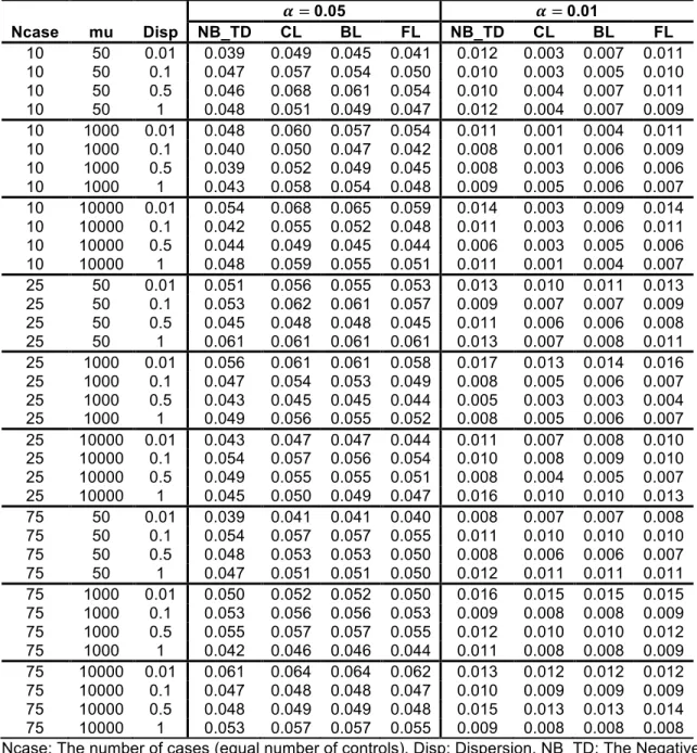
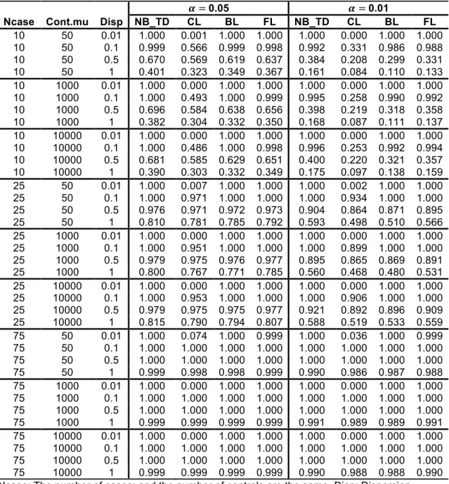
Table 2.3 Type-I error rates of the NB and logistic regressions from the balanced design 𝜶 = 0.05 𝜶 = 0.01 Ncase mu Disp NB_TD CL BL FL NB_TD CL BL FL 10 50 0.01 0.066 0.026 0.026 0.045 0.021 0.000 0.001 0.008 10 50 0.1 0.070 0.024 0.023 0.044 0.019 0.000 0.001 0.007 10 50 0.5 0.080 0.023 0.022 0.043 0.027 0.000 0.001 0.008 10 50 1 0.085 0.016 0.018 0.038 0.030 0.000 0.000 0.008 10 1000 0.01 0.066 0.023 0.023 0.044 0.018 0.000 0.000 0.007 10 1000 0.1 0.068 0.024 0.025 0.046 0.021 0.000 0.001 0.009 10 1000 0.5 0.077 0.019 0.020 0.041 0.024 0.000 0.000 0.007 10 1000 1 0.094 0.016 0.017 0.039 0.032 0.000 0.001 0.007 10 10000 0.01 0.067 0.024 0.023 0.044 0.019 0.000 0.000 0.008 10 10000 0.1 0.069 0.025 0.026 0.045 0.022 0.000 0.001 0.008 10 10000 0.5 0.076 0.022 0.022 0.044 0.025 0.000 0.001 0.007 10 10000 1 0.087 0.013 0.014 0.038 0.028 0.000 0.000 0.005 25 50 0.01 0.056 0.042 0.039 0.047 0.014 0.004 0.004 0.010 25 50 0.1 0.060 0.042 0.038 0.049 0.013 0.004 0.003 0.008 25 50 0.5 0.060 0.038 0.035 0.047 0.016 0.004 0.003 0.009 25 50 1 0.061 0.030 0.028 0.041 0.017 0.002 0.002 0.006 25 1000 0.01 0.057 0.044 0.040 0.049 0.014 0.005 0.004 0.011 25 1000 0.1 0.060 0.043 0.038 0.048 0.013 0.004 0.004 0.009 25 1000 0.5 0.062 0.040 0.037 0.047 0.018 0.004 0.004 0.011 25 1000 1 0.064 0.034 0.032 0.044 0.019 0.002 0.002 0.009 25 10000 0.01 0.059 0.045 0.041 0.049 0.015 0.005 0.005 0.010 25 10000 0.1 0.055 0.039 0.034 0.044 0.011 0.003 0.003 0.007 25 10000 0.5 0.064 0.039 0.036 0.046 0.016 0.004 0.003 0.008 25 10000 1 0.065 0.031 0.027 0.042 0.016 0.002 0.002 0.008 75 50 0.01 0.051 0.046 0.045 0.048 0.012 0.009 0.008 0.010 75 50 0.1 0.053 0.048 0.046 0.050 0.012 0.009 0.008 0.010 75 50 0.5 0.050 0.042 0.040 0.044 0.011 0.006 0.005 0.008 75 50 1 0.054 0.042 0.040 0.047 0.014 0.007 0.007 0.011 75 1000 0.01 0.054 0.050 0.048 0.051 0.012 0.009 0.008 0.010 75 1000 0.1 0.051 0.045 0.043 0.047 0.011 0.007 0.007 0.009 75 1000 0.5 0.055 0.045 0.043 0.048 0.011 0.007 0.006 0.009 75 1000 1 0.056 0.045 0.043 0.048 0.013 0.007 0.006 0.010 75 10000 0.01 0.052 0.047 0.046 0.049 0.011 0.009 0.008 0.010 75 10000 0.1 0.054 0.049 0.047 0.050 0.011 0.007 0.007 0.008 75 10000 0.5 0.056 0.047 0.045 0.050 0.011 0.007 0.007 0.009 75 10000 1 0.058 0.045 0.043 0.049 0.014 0.007 0.007 0.010 Ncase: The number of cases (equal number of controls), Disp: Dispersion, NB_TD: The Negative binomial regression with the true dispersion specified in simulation, CL: Classical Logistic

(46)

2.6.2 DA Type-I error simulation results

In most scenarios, the DA method reduces the inflation observed with NB regressions and the deflation observed with the CL, BL, and FL regressions as presented in Table 2.4. However, when the DA method is performed with CL and BL results with small sample size, conservative results, especially with the CL model, are still exhibited at alpha level 0.01. The DA method with NB and FL regressions showed well-controlled Type-I error rates at all alpha levels even