Research Archive and Digital Asset Repository
Copyright © and Moral Rights for this thesis are retained by the author and/or other copyright owners. A copy can be downloaded for personal non-commercial research or study, without prior permission or charge. This thesis cannot be reproduced or quoted extensively from without first obtaining permission in writing from the copyright holder(s). The content must not be changed in any way or sold commercially in any format or medium without the formal permission of the copyright holders.
Note if anything has been removed from thesis.
When referring to this work, the full bibliographic details must be given as follows:
Masuadi, E. (2013) Non-parametric competing risks with multivariate frailty models. PhD Thesis. Oxford Brookes University.
MULTIVARIATE FRAILTY MODELS
By
Emad Masuadi
SUBMITTED IN PARTIAL FULFILLMENT OF THE REQUIREMENTS FOR THE DEGREE OF
DOCTOR OF PHILOSOPHY AT
OXFORD BROOKES UNIVERSITY OXFORD, UNITED KINGDOM
JANUARY 2013
c
MECHANICAL ENGINEERING AND MATHEMATICAL SCIENCES
The undersigned hereby certify that they have read and recommend to the Faculty of Graduate Studies for acceptance a thesis entitled “Non-parametric Competing Risks with Multivariate Frailty Models” by Emad Masuadi in partial fulfillment of the requirements for the degree of Doctor of Philosophy.
Date: January 2013
Author: Emad Masuadi
Title: Non-parametric Competing Risks with Multivariate Frailty Models
Department: Mechanical Engineering and Mathematical Sciences Degree: Ph.D.
Permission is herewith granted to Oxford Brookes University to circulate and to have copied for non-commercial purposes, at its discretion, the above title upon the request of individuals or institutions.
Signature of Author
THE AUTHOR RESERVES OTHER PUBLICATION RIGHTS, AND NEITHER THE THESIS NOR EXTENSIVE EXTRACTS FROM IT MAY BE PRINTED OR OTHERWISE REPRODUCED WITHOUT THE AUTHOR’S WRITTEN PERMISSION.
THE AUTHOR ATTESTS THAT PERMISSION HAS BEEN OBTAINED FOR THE USE OF ANY COPYRIGHTED MATERIAL APPEARING IN THIS THESIS (OTHER THAN BRIEF EXCERPTS REQUIRING ONLY PROPER ACKNOWLEDGEMENT IN SCHOLARLY WRITING) AND THAT ALL SUCH USE IS CLEARLY ACKNOWLEDGED.
Table of Contents v
List of Tables viii
List of Figures xi
Abstract xii
Acknowledgements xiii
Symbols and abbreviations xiv
1 Introduction 1
2 Survival Analysis 5
2.1 Definitions . . . 6
2.2 Censoring . . . 8
2.3 Non-parametric survival distribution . . . 9
2.3.1 Life-table estimator . . . 10
2.3.2 Product-limit estimator . . . 10
2.4 Parametric survival distribution . . . 11
2.4.1 Exponential distribution . . . 12 2.4.2 Weibull distribution . . . 12 2.4.3 Gamma distribution . . . 13 2.4.4 Log-Normal distribution . . . 13 2.4.5 Log-Logistic distribution . . . 14 2.5 Likelihood function . . . 20
2.6 Proportional hazard models . . . 21
2.7 Accelerated failure time models . . . 22
2.8 Breast cancer recurrence data . . . 24
3.2 Linear mixed models . . . 28
3.3 Model Identifiability . . . 30
3.4 Univariate frailty models . . . 30
3.4.1 Gamma frailty model . . . 33
3.4.2 Inverse Gaussian frailty model . . . 34
3.4.3 Log-Normal frailty models . . . 36
3.4.4 Weibull hazard with Log-Normal frailty . . . 37
3.4.5 Non-parametric frailty models . . . 40
3.5 Univariate simulations . . . 41
3.6 Results on breast cancer recurrence data . . . 46
3.7 Summary . . . 54
4 Multivariate frailty in competing risks models 56 4.1 Introduction . . . 56
4.2 Shared frailty models . . . 58
4.3 Correlated frailty models . . . 60
4.4 Competing risks models . . . 62
4.5 Frailty in Competing Risks Models . . . 63
4.6 Correlated Gamma frailty model . . . 66
4.7 Correlated Inverse Gaussian frailty model . . . 69
4.8 Multivariate Inverse Gaussian frailty model . . . 73
4.8.1 Inverse Gaussian frailty model . . . 73
4.9 Multivariate Log-Normal frailty model . . . 75
4.9.1 Cholesky decomposition . . . 75
4.9.2 Weibull competing risks with Log-Normal frailty model . . . 79
4.10 Competing risks with non-parametric frailty model . . . 79
4.11 Multivariate simulations . . . 81
4.11.1 Bivariate Inverse Gaussian frailty of competing risks model . . . 82
4.11.2 Bivariate Log-Normal frailty of competing risks model . . . 84
4.11.3 Multivariate Log-Normal frailty of competing risks model . . . 86
4.11.4 Bivariate non-parametric frailty of competing risks model . . . 88
4.12 Results on breast cancer recurrence data . . . 90
4.12.4 Clinical results . . . 103
4.13 Summary . . . 105
5 Frailty and finite mixture 106 5.1 Introduction . . . 106
5.2 Frailty as a finite mixture . . . 107
5.2.1 Finite mixture of Gamma frailty model . . . 109
5.2.2 Finite mixture of Inverse Gaussian frailty model . . . 109
5.2.3 Finite mixture of Log-Normal frailty model . . . 110
5.3 Finite mixture of correlated Inverse Gaussian frailty model . . . 110
5.4 Simulations . . . 112
5.5 Summary . . . 120
6 Conclusions 121 6.1 Introduction . . . 121
6.2 Concluding Remarks . . . 121
6.3 Limitations and future research . . . 123
Appendices 125 A Data 126 A.1 Variables in the model . . . 126
A.2 Variables by risks . . . 128
A.3 Data analysis without frailty . . . 129
A.4 Non-parametric frailty . . . 130
A.5 Log-Normal frailty . . . 131
B Correlated frailty 134 B.1 Correlated Gamma frailty . . . 134
B.2 Correlated Inverse Gaussian frailty . . . 135
C Gauss code 136
2.1 Some common parametric survival distribution along with their associated functions . . . 19 2.2 Some distributions ofεiand their corresponding distributions ofT in modelling
AFT. . . 24
3.1 Simulation data of Weibull baseline hazard generated with Log-Normal frailty and fitted by Log-normal, 600 data sets each with sample sizes of 500 and 5000. 43 3.2 Log-Normal, Gamma and Inverse Gaussian frailty model with Weibull baseline
hazard and four covariates simulated data fitted by Log-Normal frailty, 600 data sets each with sample sizes of 500 and 5000. . . 44 3.3 Log-Normal, Gamma, Inverse Gaussian and arbitrary frailty model with Weibull
baseline hazard and four covariates simulated data, fitted by non-parametric frailty, 600 data sets each with sample sizes of 500 and 5000. . . 45 3.4 Patients status at time of first recurrence. . . 46 3.5 Independent variables included in the models. . . 47 3.6 Results of breast cancer data: died from breast cancer with the cox
propor-tional hazard, Weibull hazard and Weibull-Gamma frailty. Parameters’ esti-mates with their standard error in parentheses. . . 51 3.7 Results of breast cancer data: Died from breast cancer assuming different
frailty distributions. Parameters’ estimates with their standard error in paren-theses. . . 53 3.8 Non-parametric models with different mass points. . . 54
4.1 Univariate, multivariate and competing risks data presentation. . . 64 4.2 Bivariate Inverse Gaussian frailty model with Weibull baseline hazard and two
sets of covariates simulated data, 500 data sets each with sample sizes of 1000 and 5000. . . 83
5000. . . 85 4.4 Trivariate Log-Normal frailty model with Weibull baseline hazard and two
covariates simulated data, 500 data sets each with sample sizes of 1000 and 5000. . . 87 4.5 Log-Normal, Gamma and Inverse Gaussian frailty model with Weibull baseline
hazard and two covariates simulated data fitted non-parametrically, 500 data sets each with sample sizes of 500 and 5000. . . 89 4.6 Results of breast cancer data: local recurrence. Parameters’ estimates with
their standard error in parentheses. . . 91 4.7 Results of breast cancer data: regional recurrence. Parameters’ estimates with
their standard error in parentheses. . . 93 4.8 Results of breast cancer data: metastasis. Parameters’ estimates with their
standard error in parentheses. . . 95 4.9 Results of breast cancer data: died from breast cancer. Parameters’ estimates
with their standard error in parentheses. . . 97 4.10 Results of breast cancer data: died from other causes. Parameters’ estimates
with their standard error in parentheses. . . 99 4.11 Deviances of testing for merging competing risks. . . 100
5.1 Log-Normal, Gamma, Inverse Gaussian and arbitrary frailty models with Weibull baseline hazard and four covariates simulated data estimated by Gamma frailty, 500 data sets each with sample sizes of 500 and 5000. . . 113 5.2 Log-Normal, Gamma, Inverse Gaussian and arbitrary frailty models with
Weibull baseline hazard and four covariates simulated data estimated by mix-ture of Gamma frailty, 500 data sets each with sample sizes of 500 and 5000. 114 5.3 Log-Normal, Gamma, Inverse Gaussian and arbitrary frailty models with
Weibull baseline hazard and four covariates simulated data estimated by In-verse Gaussian frailty, 500 data sets each with sample sizes of 500 and 5000. 115
ture of Inverse Gaussian frailty, 500 data sets each with sample sizes of 500 and 5000. . . 116 5.5 Log-Normal, Gamma, Inverse Gaussian and arbitrary frailty model with Weibull
baseline hazard and four covariates simulated data estimated by mixture of Log-Normal frailty, 500 data sets each with sample sizes of 500 and 5000. . . 117 5.6 Bivariate Log-Normal, Gamma and Inverse Gaussian frailty model with Weibull
baseline hazard and two covariates simulated data fitted by mixture of bivari-ate Inverse Gaussian, 500 data sets each with sample sizes of 500 and 5000. . 118
A.1 Independent variables by recurrence type. . . 128 A.2 Weibull baseline hazard model without frailty for all failure types. . . 129 A.3 Breast cancer Weibull hazard with non-parametric frailty using different
num-ber of mass points. . . 130 A.4 Breast cancer Weibull hazard with Log-normal frailty using different number
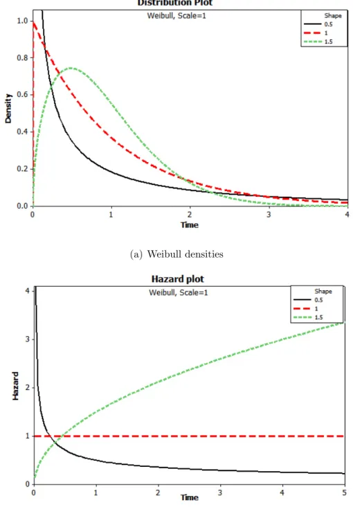
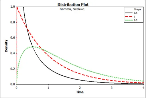
2.1 Weibull densities and hazards with scale parameterλ = 1 and shape parameter α= (0.5,1,1.5) . . . 15 2.2 Gamma densities and hazards with scale parameterλ= 1 and shape parameter
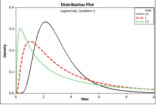
α= (0.5,1,1.5) . . . 16 2.3 Log-Normal densities and hazards with location parameter (µ= 1) and shape
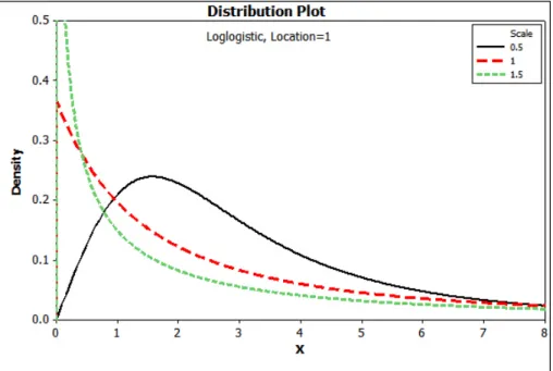
parameter(α = (0.5,1,1.5)) . . . 17 2.4 Log-Logistic densities and hazards with scale parameter λ = 1 and shape
parameterα = (0.5,1,1.5) . . . 18
3.1 Inverse Gaussian densities with scale parameter λ = 1 and shape parameter α= (0.5,1,1.5,5) . . . 35 3.2 Weibull hazards of died from breast cancer for independent and frailty models. 50
This research focuses on two theories: (i) competing risks and (ii) random effect (frailty) models. The theory of competing risks provides a structure for inference in problems where cases are subject to several types of failure. Random effects in competing risk models consist of two underlying distributions: the conditional distribution of the response variables, given the random effect, depending on the explanatory variables each with a failure type specific random effect; and the distribution of the random effect. In this situation, the distribution of interest is the unconditional distribution of the response variable, which may or may not have a tractable form. The parametric competing risk model, in which it is assumed that the failure times are coming from a known distribution, is widely used such as Weibull, Gamma and other distributions. The Gamma distribution has been widely used as a frailty distribution, perhaps due to its simplicity since it has a closed form expression of the unconditional hazard function. However, it is unrealistic to believe that a few parametric models are suitable for all types of failure time.
This research focuses on a distribution free of the multivariate frailty models. Another approach used to overcome this problem is using finite mixture of parametric frailty especially those who have a closed form of unconditional survival function. In addition, the advantages and disadvantages of a parametric competing risk models with multivariate parametric and/or non-parametric frailty (correlated random effects) are investigated. In this research, four main models are proposed: first, an application of a new computation and analysis of a multivariate frailty with competing risk model using Cholesky decomposition of the Log-normal frailty. Second, a correlated Inverse Gaussian frailty in the presence of competing risks model. Third, a non-parametric multivariate frailty with parametric competing risk model is proposed. Finally, a simulation study of finite mixture of Inverse Gaussian frailty showed the ability of this model to fit different frailty distribution. One main issue in multivariate analysis is the time it needs to fit the model. The proposed non-parametric model showed a significant time decrease in estimating the model parameters (about 80% less time compared the Log-Normal frailty with nested loops). A real data of recurrence of breast cancer is used as the applications of these models.
First of all, I would like to thank God, the Almighty, for having made everything possible by
giving me strength and courage to write this dissertation.
I would like to thank my supervisor Dr. Reza Oskrochi, for his many suggestions, guidance
and constant support during this research. I am also tremendously grateful to Prof. Kilani
Ghodi, my co-advisor for his critical suggestions which enrich the entire thesis. My deepest
thank to my second co-advisor Dr. Hooshang Izadi for his valuable suggestions and comments.
I would like to thank the exam committee Dr.Hafiz.T.A.Khan and Dr.Robert Beale for their
remarkable suggestions. Of course, I am grateful to my parents, my wife and my kids for
their patience andlovethroughout the years of my study and without them this work would never have come into existence. Finally, I wish to thank the following: Dr. Omar Al Atari
for the proof reading of this dissertation. Thanks to Prof. Yahia El-Bassiouni for his endless
support at the academic as well as the professional level.
Oxford, UK Emad Masuadi
AFT accelerated failure time
c.d.f cumulative distribution function
E[Z] the expected value of the random variableZ
h(t) hazard function
c.h.f cumulative hazard function H(t) cumulative hazard function HR hazard ratio
L(θ;ti) likelihood fuction
L the Laplace transformation LMMs Linear mixed models p.d.f probability density function p.m.f probability mass function PH proportional hazards
S(t) survival function
T ∼EXP(λ) Exponential distribution scale parameter λ
T ∼Γ(α, λ) Gamma distribution with shape parameter α and scale parameter λ
T ∼LogL(α, λ) Log-Logistic distribution with shape parameter α and scale parameter λ T ∼IG(α, λ) Inverse Gaussian distribution with shape parameterα and scale parameter λ T ∼LogN(µ, σ2) Log-Normal distribution with location parameterµand scale parameterσ
T ∼W eib(α, λ) Weibull distribution with shape parameter α and scale parameter λ
Zk×1 ∼M IG(β, µ,Ω) Multivariate Inverse Gaussian distribution with parametersβ, µ,Ω V[Z] the variance of the random variable Z
Statisticians, like artists, have the bad habit of falling in love with their models. (George Box)
Introduction
The term survival analysis summarises statistical models and methods for analysing lifetime
data or time-to-event data. These models are frequently employed in a variety of disciplines
including Bio-statistics, Epidemiology, Engineering, Social Sciences and Economics. Survival
analysis differs from other statistical procedures in many features; one of these features
is the incompleteness of the survival times due to the censoring mechanism that gives a
mixture of discrete and continuous data. Another difference is the shape of the distribution
of the survival times that are non-negative random variables and usually skewed to right.
The proportional hazards models (PH) by Cox (1972) which assume that covariates have a
multiplicative effect on the hazard have dominated survival analysis. In addition, accelerated
failure time models are also used for the analysis of survival data by modelling the survival
time it-self and the covariates are assumed to act directly on it. During recent decades, these
models have been extended to become suitable for handling more complex survival data so
as to include frailty models and competing risks models. They provide a powerful tool to
analyse models with repeated measures, clustered survival data and multiple types of failure.
One of the main assumptions in analysing survival data is that all subjects have the same risk
of failure, which means that populations are homogeneous. However, this is usually not true
as different subjects could have different hazards. In univariate survival data, frailty models
important covariates in the model. In multivariate survival data, frailty models are used
when there are repeated measures or clustering. Repeated data occur in case of longitudinal
data or multiple recurrences of an event for the same individual. Competing risks models are
another form of multivariate survival data where the censoring variable is decomposed into
different variables. For each type of failure the subject experiences the event of that failure
or is censored.
Competing risks with frailty models frequently arise in a number of substantive scientific
research areas, particularly within the Social Sciences, Bio-statistics and Epidemiology. These
models combine two theories: (i) competing risks and (ii) random effect (or frailty) models.
The theory of competing risks provides a structure for reference to problems where cases are
subject to several types of failure, i.e. multiple causes of failure. There are two approaches
to analyse competing risks models in the literature. One places emphasis on cause specific
hazard functions and sub-distribution functions, while the other uses the concept of latent
failure times, where there is an inherent failure time for each type of failure, and only one
such time, the smallest, is observable. Both approaches arrive at the same inference, using
different notation (Kalbfleisch and Prentice, 2002 and Kundu, 2004). The concept of latent
failure times is the one employed in this thesis.
Random effects in competing risk models consist of two underlying distributions: the
conditional distribution of the response variables (i.e. failure types), given the random effect,
depending on the explanatory variables each with a failure type specific random effect; and the
distribution of the random effect in the population (i.e. frailty distribution). In this situation,
the distribution of interest is the unconditional distribution of the response variables which
Due to its simplicity, the parametric competing risk model where the failure times have a
known distribution with monotonically increasing or decreasing baseline hazard and known
distribution of random effect, is widely used in practice (Hougaard, 2000, Lambert et al.,
2004 and Oskrochi and Crouchley, 2004), but it is unrealistic to believe that a few parametric
models are suitable for all types of failure time. Unlike the parametric models, a distribution
free model for the random effect in which only the baseline hazard follows a specific
distribution will be less demanding in term of assumptions and would be more robust. In
this situation the unconditional distribution of the competing risks does not have a tractable
form and hence a more complex non-linear multivariate optimisation procedure is needed
for parameter estimation (Oskrochi and Davies, 1997). One should differentiate between
the ways frailty introduced into the model. In univariate failure time, frailty is included
to accommodate heterogeneity between individuals. When individuals in the same group
or cluster are assumed to share the same frailty then it accommodates the heterogeneity
between clusters not individuals, the so-called shared frailty. Another way to include frailty
is by assuming different frailties for different individuals or for different competing risks.
In correlated frailty models, frailties are correlated through a covariance matrix and have
the same set of marginal distributions but not coming from a multivariate distribution. In
multivariate frailty models, frailties have a multivariate distribution with a general correlation
structure between the frailties.
This study will investigate the methodology and the applications of competing risk models
with multivariate frailty. In the first stage, the Chloeskey decomposition is applied in
analysing competing risks model for censored survival data with multivariate Log-Normal
frailty to a real data of breast cancer. In the second stage, a correlated Inverse Gaussian
frailty as well as a multivariate Inverse Gaussian frailty is proposed. In the third stage, a
is proposed. In the last stage, a finite mixture of Inverse Gaussian frailty is proposed. The
advantages and disadvantages of competing risk model with non-parametric and/or
semi-parametric multivariate frailty is compared using simulations data as well as real data.
In Chapter 2, a general introduction to survival analysis and its main characteristics is
summarized along with a description of a set of survival data on the recurrence of breast
cancer in the UK, which is used throughout the thesis to demonstrate the development of
the proposed models. In Chapter 3, a literature review of the univariate frailty models is
conducted. Chapter 4 generalises these models to suite correlated and multivariate frailty
models in the presence of competing risks in cases of parametric as well as non-parametric
frailty. In chapter 5, a different approach is used to fit frailty models by decomposing the
frailty distribution as a finite mixture model (semi-parametric model). Finally, chapter 6
concludes the main results and discusses the advantages and disadvantages of the proposed
Survival Analysis
The term ”survival analysis” is used for describing data that measure the time to some event.
The statistical analysis of survival data or ’time-to-event’ has applications in disciplines as
diverse as Medicine, Social Sciences, Engineering, Epidemiology, Economics, as well as many
others. Time-to-event could mean the time until some electrical component fails, time of
remission of a certain disease after treatment, or time from graduation until employment.
These applications have ensured that survival analysis has expanded rapidly in the last three
decades. In this study, the applications are within the biomedical framework where real data
from medical fields are used and our subjects are individuals. Two features of survival data
make them differ from the data used in classical methods (e.g. general linear models). First,
there is a mixture of discrete and continuous variables. The time-to-event is the continuous
part and the censoring is the discrete part. An individual is said to be censored if s/he does
not experience the time of interest before the end of the study: for example, a patient with
breast cancer may stay alive after the termination of the study. Second, in classical methods,
the dependent variable is modelled through a link function with a linear combination of the
explanatory variables. In survival analysis, the model is built either by the hazard function,
which represents the failure rate at time t; for example, proportional hazard model (PH) Cox
(1972), or by the survival function which represents the probability of surviving beyond time
2.1
Definitions
2.1.1 Definition. Let T be a non-negative random variable that represents the survival time (failure time, lifetime), of a subject, with probability density function (p.d.f)f(t), and
cumulative distribution function (c.d.f) F(t) = Pr(T ≤t).
IfT is absolutely continuous then the probability density function is
f(t) = lim
∆t→0+
P(Failure occurs in[t, t+ ∆t))
∆t .
2.1.2 Definition. The survival function S(t) = Pr(T ≥ t), is the probability of an individual surviving beyond time t, or more generally, the probability that the event of
interest has not occurred by duration t.
From the definition, if it is a continuous random variable then,
S(t) = Pr(T ≥t) = Z ∞
t
f(u)du.
IfT is discrete with mass points at tj with probability mass function (p.m.f)fj =P(T =tj)
then, for tj ≤t < tj+1,
S(t) =X
i≥j
f(ti).
2.1.3 Definition. If T is an absolutely continuous random variable then, the hazard function is given by h(t) = lim ∆t→0 Pr(t≤T < t+ ∆t|T ≥t) ∆t = f(t) S(t), (2.1.1)
time t. If T is a discrete random variable, then the hazard function is given by h(t) =P(T ≥t|T =t) = Pr(T =t) P(T ≥t) = f(t) S(t−), where S(t−) = lim x→t−S(x) (t
−: from left). Moreover,
S(t) = j Y i=1 S(ti+1) S(ti) = j Y i=1 S(ti)−fi S(ti) = j Y i=1 1− fi S(ti) and hence, S(t) = j Y i=1 (1−h(ti)).
2.1.4 Definition. If T is an absolutely continuous random variable then, the cumulative hazard function c.h.f is H(t) = Z t 0 h(u)du=−logS(t). (2.1.2) Or equivalently, S(t) =e−H(t) = exp − Z t 0 h(u)du .
The p.d.ff(t) can be written in terms of the hazard and the cumulative hazard function,
f(t) = h(t)exp[−H(t)].
H(t) =X
i≤j
h(ti)
Sometime it is desirable to find the mean or the expected lifetime of subjects, for instance if
T is a continuous random variable with p.d.f f(t) then expected value of T is
µ= Z ∞
0
tf(t)dt.
Another way to get this expected value is by integrating the survival function, assuming that
the event of interest is bound to occur (i.e. S(∞) = 0)
µ= Z ∞
0
S(t)dt.
2.2
Censoring
As mentioned above, censoring is one of the reasons that survival analysis differs from
standard statistical analysis, so censored data are those observations whose time-to-event is
not observed before the end of the study. There are three different mechanisms of censoring:
type I, type II, andrandom censoring. Intype I censoring, a sample of n subjects is followed for a specific time T∗ under the control of the researcher, so that the total duration of the
study is fixed whilst the number of subjects who experience the event of interest is random,
the actual failure timeti cannot be observed ifti > T∗. This type of censoring is usually used
in medical applications. The opposite of this mechanism, type II censoring, occurs when a sample of n subjects is followed until the failure time of the first r(r ≤n) of the subjects is observed. This type of censoring is usually used in industrial applications. Another possible
mechanism of censoring is random censoring, where each subject has associated with it a potential censoring time Ci and a potential survival time Ti, which are usually assumed to
be independent of one another (the so-called independent censoring). This type of censoring
will be the main censoring mechanism that is used within this thesis. Usually, the observed
variables are Yi = min(Ti, Ci), and the indicator variable δi.
Yi = ( Ti if Ti ≤Ci Ci if Ti > Ci , and δi = ( 1 if Ti ≤Ci 0 if Ti > Ci.
The observed data takes the form, (y1, δ1), ...,(yn, δn), and possibly some factors (independent
variables). There are three different kinds of censoring, right-censoring, left-censoring, and
interval-censoring:
Right-censoring: when subjects leave the study or the study ends before observing their survival (failure) time. It is only known that their survival timeTi lies in an interval (t,∞).
Throughout this thesis, right-censoring is assumed.
Left-censoring: when subjects experience the event (failure) before a certain duration. It is only known that their survival timeTi lies in an interval [0, t).
Interval-censoring: when it is not clear when the event occurred. It is only known that the time-to-event occurred within some interval [t1, t2). For more information see Lee and Wang
(2003).
2.3
Non-parametric survival distribution
When it is difficult to determine the distribution of the survival time, or no assumption
about the distribution is made, non-parametric or distribution-free survival time approaches
represent viable alternatives. In this case, the empirical distribution function is used to
estimate the survival function assuming that all subjects have experienced failure (i.e., no
censored data). The empirical survival function is given by
˜
S(t) = N umber of subjects with survival times≥t N umber of subjects in the data set .
The following subsections give a briefly review of the two most popular estimators of the
survival function using both censored and uncensored data.
2.3.1
Life-table estimator
In the case of some subjects with censored time, the empirical function is not applicable any
more. Life-table estimator divides the study time into, usually equal intervals. The interval
width and number of intervals varies from one study to another depending on the length
of the study and the number of observations. Suppose that (t1, ..., tk) are the boundaries of
these intervals and letdi,ci andni denote the number of failures, number of censored subjects
and number of subjects who are at risk during the interval [ti, ti+1) respectively. Assuming
that the censoring is uniformly distributed along the interval, the average number of subjects
at risk during the interval [ti, ti+1) is n∗i =ni−ci/2, and hence the probability of failure is
di/n∗i. For t ∈ [tj, tj+1), and j = 1, ..., k, the life-table estimator of the survival function is
given by j Y i=1 1− di n∗i .
2.3.2
Product-limit estimator
Kaplan and Meier (1958) provided a special case of the life-table estimator, where the interval
boundaries are chosen so that there is at least one failure. Suppose that (t(1), ..., t(m))are the
ordered time points in which there is at least one failure so that,t(1) < t(2) <· · ·< t(m). For
by j Y i=1 1− di ni .
2.4
Parametric survival distribution
Although the non-parametric methods mentioned above are widely used in applications and
do not require any specific assumptions they are unsuitable for handling complex data sets
with explanatory variables, and if the distribution of the survival time is known, the inferences
will be more accurate. This section reviews some of the most commonly used distributions for
survival time. Actually, any non-negative random variable, whether discrete or continuous,
can be used to describe the survival time, while in this thesis our focus will be on continuous
distributions. Other random variables defined over the real line can be used say,x∈(−∞,∞) such thatx=log(t) or equivalentlyt=ex. There are some distributions that have been used
frequently in the literature of survival analysis, such as the Exponential, Weibull, Gamma,
Log-Normal and Log-Logistic distributions. For each distribution, the probability density
function, survival function, hazard function, expected value and the variance of survival time
are summarised in Table 2.1.
The Log-Normal and the Gamma distributions are generally less convenient computationally,
but are still frequently applied, as well as non-parametric approaches, such as the product
limit estimator suggested by Kaplan and Meier (1958) and related techniques. The
advantages and disadvantages of different parametric, semi-parametric and non-parametric
models as methodologies for statistical inference can be found in books such as Kalbfleisch
and Prentice (2002), Miller (1981), Lawless (1982), Cox and Oakes (1984) and Klein and
2.4.1
Exponential distribution
The simplest distribution for survival time is the Exponential distribution (T ∼ EXP(λ)), especially used in reliability analysis in engineering applications. The p.d.f, the mean and
the variance of T are given in Table 2.1. It is used to model data with a constant failure
rate (indicated by the hazard plot which is simply equal to a constant). The exponential
distribution is a member of the exponential family. It has a unique property of “lack of
memory”, because of its constant hazard rateλ. The probability to failure within a particular
time interval depends only on the length, not on the location of this interval. In real-world
applications, the assumption of a constant rate is rarely satisfied.
2.4.2
Weibull distribution
The Weibull model is the most widely used parametric survival model. The Weibull
distribution was introduced by Weibull (1939); it is an important generalisation of the
exponential distribution with two positive parameters T ∼W eib(α, λ), where αis the shape parameter and λ is the scale parameter. Its first parameter allows different failure rates; if
it is less than one this indicates a decreasing hazard function while a value more than one
indicates an increasing hazard function, but if it is one then the distribution becomes the
exponential distribution and the hazard function is constant. Figure 2.1 describes the density
and the hazard curves of the Weibull distribution with a scale parameter that equals one with
different values of the shape parameter . The Weibull model also has another property in
the sense that if the plot of log(−log( ˆS(t))) against log(t) shows a linear trend, that would suggest Weibull model. ˆS(t) is the empirical survival function which can be obtained the by
2.4.3
Gamma distribution
Another possible distribution of the survival time is the Gamma distribution T ∼ Γ(α, λ) with two positive parameters: α the shape parameter and λ1 the scale parameter. Like the
Weibull distribution, it includes the Exponential distribution as a special case when α = 1.
The Gamma distribution is of limited use in survival analysis because the Gamma models
do not have closed-form expressions neither for the survival nor the hazard function, if α is
not an integer since both include the incomplete Gamma integral (Ifα is an integer then the
distribution reduces to Erlang distribution). Its maximum likelihood estimation is difficult to
get and involves incomplete Gamma integrals. This requires additional numerical calculations
in parameter estimation. It can be shown that the limit of its hazard as time goes to infinity
is equal to the shape parameter ( lim
t→∞h(t) = λ). The Gamma hazard increases monotonically
if α > 1, from a value of zero at the origin to a maximum of λ; and is constant if α = 1;
and decreases monotonically if α < 1, from infinity at the origin to an asymptotic value of
λ. Figure 2.2 describes the density and the hazard curves of the Gamma distribution with a
scale parameter which equals one with different values of the shape parameter.
2.4.4
Log-Normal distribution
A random variable has a log-Normal distribution if the logarithm of the random variable is
normally distributed T ∼ LogN(µ, σ2) if and only if log(T) ∼ N(µ, σ2). The log-Normal distribution is self-replicating under multiplication and division. That is, multiplying or
dividing Log-Normal random variables will result in Log-Normal distributions. The hazard
function of the log-Normal differs from the previous two distributions; it starts from zero
at t = 0, increases to a maximum and then decreases and approaches zero as time goes to
unsuitable to model lifetime data in most medical applications. However, the Log-Normal
distribution can be very useful for representing lifetimes for situations with non-monotonic
hazards such as the analysis of electrical insulation or time to occurrence of lung cancer
among smokers. Figure 2.3 shows the density and the hazard curves of the Log-Normal
distribution with a location parameter which equals one with different values of the shape
parameter. It is similar to the Gamma distribution in the complexity of the hazard function
since numerical integration needs to be used to fit the distribution.
2.4.5
Log-Logistic distribution
The Log-Logistic distribution is the probability distribution of a random variable whose
logarithm has a logistic distribution T ∼ LogL(α, λ). It is one of the parametric survival time models in which the hazard rate may be decreasing (if λ ≤ 1), increasing, or hump-shaped (if λ > 1), that is, it initially increases and then decreases. Figure 2.4 describes the
density and the hazard curve of the log-logistic distribution with scale parameter equals one
with different values of the shape parameter. It has also another property that if the plot of
the logit of the survival function S(t), (log(1−SS(t()t))) against log(t) has a linear trend then it
(a) Weibull densities
(b) Weibull hazards
Figure 2.1: Weibull densities and hazards with scale parameter λ = 1 and shape parameter
(a) Gamma densities
(b) Gamma hazards
Figure 2.2: Gamma densities and hazards with scale parameter λ = 1 and shape parameter
α= (0.5,1,1.5)
(a) Log-Normal densities
(b) Log-Normal hazards
Figure 2.3: Log-Normal densities and hazards with location parameter (µ = 1) and shape parameter(α= (0.5,1,1.5))
(a) Log-Logistic densities
(b) Log-Logistic hazards
Figure 2.4: Log-Logistic densities and hazards with scale parameter λ= 1 and shape parameter
α= (0.5,1,1.5)
T able 2.1: Some comm on parametric surviv al distribution along with their asso ciated functions Distribution Probabilit y densit y function f ( t ) Surviv al function S( t ) Hazard function h( t )
Cum. hazard function H(
t ) Mean E( T ) V ariance V ar ( T ) Exp onen tial λexp ( − λt ) , λ > 0 ,t ≥ 0 exp ( − λt ) λ λt (1/ λ ) 1/ λ 2 W eibull α λt α − 1 exp ( − λt α ) , α ,λ > 0 , t ≥ 0 exp ( λt α ) α λt α − 1 λt α Γ(1+(1/ α )) λ (1/ α ) Γ(1+2/ α ) − Γ(1+1/ λ (2/ α ) Gamma 1 Γ( α ) λ α t α − 1 exp ( − λt ) , α ,λ > 0 ,t ≥ 0 1 − I α( λt ) ∗ λ αt α − 1exp ( − λt ) (1 − Iα ( λt ))Γ( α ) —– α λ α 2λ Log-Normal exp ( 1 2 σ 2 ( ln ( t ) − µ ) 2 ) tσ √ 2 π , σ > 0 ,t ≥ 0 1 − Φ ln ( t ) − µ σ ∗∗ f ( t ) S ( t ) —– exp ( µ + σ 2 ) 2 ( e σ 2 − 1) e ( σ 2 Log-Logistic αλt α − 1 (1+ λt α) 2 , α ,λ > 0 ,t ≥ 0 1 1+ λt α αλt α − 1 1+ λt α ln(1 + λt α ) π csc( π /α ) αλ (1 /α ) , if α > 1 2 απ csc( 2 π)α − π 2 α 2λ (2 /α if α > 2 Iα ( t ) = R t (1 0 / Γ( α )) x α − 1 e − x dx is the incomplete Gamma function, **Φ( · ) is the cum ulativ e distribut ion fu nction Normal distri bution.
2.5
Likelihood function
In order to estimate the parameters involved in the survival analysis models, the likelihood
function is usually used. Since the observed data takes the form,(t1,δ1), ...,(tn, δn), where
(ti, δi) are respectively the survival time and the censoring indicator for the ith individual,
the likelihood function L(θ;ti) is given by
L(θ;ti) = n
Y
i=1
[f(ti)]δi[S(ti)]1−δi.
Using the relation in (2.1.2) the likelihood function becomes
L(θ;ti) = n
Y
i=1
[h(ti)]δiS(ti). (2.5.1)
The maximum likelihood estimator of θ is the value in the parameter space that maximises
the likelihood function or equivalently the log-likelihood function which is given by
`(θ;ti) = n
X
i=1
δilog[h(ti)] + log[S(ti)]. (2.5.2)
Example 2.1 Assume the survival times follow the Weibull distribution T ∼ W eib(α, λ), then from Table 2.1, the probability density function, the hazard, and the survival function
are given by
f(t) = αλtα−1exp(λtα), h(t) =αλtα−1, S(t) =exp(λtα).
`(λ, α;ti) = n X i=1 δilog[αλtα−i 1] +λt α i, and consequently, `(λ, α;ti) =rlog(αλ) + (α−1) n X i=1 δilogti−λ n X i=1 tαi, wherer=Pn
i=1δi is the number of uncensored individuals. Differentiating the log-likelihood
function and setting it to zero, the maximum likelihood estimators of λ and α are given by
ˆ λ= Pnr i=1tαiˆ , and r ˆ α + n X i=1 δilogti−ˆλ n X i=1 tαiˆlogti = 0.
The values of ˆλand ˆαcan be found by an iterative numerical procedure such as the
Newton-Raphson algorithm.
2.6
Proportional hazard models
Many studies focus on determining the risk factors affecting the survival times of individuals
or subjects. Cox (1972) introduced the proportional hazard model (PH) in order to estimate
the effects of such risk factors or covariates influencing survival time data. It assumes that
the covariates have a multiplicative effect on the hazard. The proportional hazard model is
the most popular model for survival data and has been used extensively in the literature.
The proportional hazard model is given by
h(ti,xi) =h0(ti) exp(x
0
iβ). (2.6.1)
If the proportionality assumption is not satisfied, an alternative way to include the effect of
covariates is using additive models. The hazard function then takes the form
h(ti,xi) =h0(ti) +x
0
iβ. (2.6.2)
For more details, see (Lin and Ying, 1994) and (Beamonte and Bermdez, 2003). A more
general model that includes both types is called an additive-multiplicative model (Lin and
Ying, 1995).
Example 2.2 Assume the survival times follow the Weibull distribution T ∼ W eib(α, λ). Then h0(ti) =αtα−i 1, and under the assumption of multiplicative hazard model, and setting
λ= exp(x0iβ) and r =Pn i=1δi,
h(ti,xi) =αtα−i 1exp(x
0
iβ), and S(ti,xi) = exp(−tαi exp(x
0
iβ)).
Consequently, the log-likelihood is given by
`(β, α;ti) = r(log(α) +x 0 iβ) + (α−1) n X i=1 δilogti− n X i=1 tαi exp(x0iβ). (2.6.3)
2.7
Accelerated failure time models
Another way to estimate the effect of covariates on the survival time is through modelling the
survival time by accelerated failure time (AFT). The covariates are assumed to act directly
on survival times. The proportional hazard model is given by
S(ti,xi) = S0(tiexp(x
0
where S0(t) is the baseline survival function corresponding to the survival function of a
subject with covariate variables xi equal to 0. Another way to represent (2.7.1) is using the
survival time,
T =T0exp(x
0
iβ),
where T0 has survival function S0(t). The AFT model assumes the effect of covariates is
multiplicative with respect to survival time. The AFT models are similar to the usual linear
regression model
log(Ti) =x
0
iβ+σεi,
whereβis the unknown regression coefficient andx0iis the vector of observed covariates. The
random errors εi is assumed to be independently and identically distributed with the mean
zero and standard deviation one. If there are no censored data, the model can be readily
estimated by ordinary least squares. One can simply generate a new variable, Y = log(T),
and use the linear regression model with Y as the dependent variable. If the error εi is
normally distributed, the OLS estimates will also be maximum likelihood estimates of the
model parameters. Survival data usually have at least some censored observations, and
these are difficult to handle with OLS. Alternatively, one can use Maximum Likelihood
Estimation (MLE) method with different distribution assumption. For each distribution of
εi, there is a corresponding distribution for T. For instance, if the survival times follow the
Weibull distribution T ∼ W eib(α, λ), then y = log(T) has the extreme-value distribution y∼ext(a, b),where a= logλ and b= 1/α , therefore,
`(β, b;yi) =−rlog(b) + n X δi yi−x 0 iβ b − n X exp yi −x 0 iβ b .
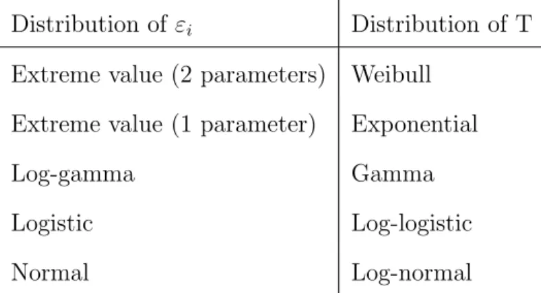
The following table lists some distributions of εi and their corresponding distributions ofT.
Distribution of εi Distribution of T
Extreme value (2 parameters) Weibull
Extreme value (1 parameter) Exponential
Log-gamma Gamma
Logistic Log-logistic
Normal Log-normal
Table 2.2: Some distributions ofεi and their corresponding distributions ofT in modelling AFT.
2.8
Breast cancer recurrence data
This section describes a set of survival data on the recurrence of breast cancer in the UK
which will be used throughout the thesis to demonstrate the development of the proposed
models. The data used in this study was collected and provided by Research division of
Christie Hospital in Manchester U.K. and includes more than 2850 women who were referred
to the Christie Hospital, U.K. during 1985 and 1995, by their GPs with diagnosis of breast
cancer. The data also includes the subsequent monitoring of these women up to 2001. This is
an observational data set, hence, no randomisation or clinical trial was involved. Recurrence
in this study is defined as clinical recurrence of breast cancer (i.e. after remission). The
data were checked for values that were out of range, incorrect sequence of events or dates,
and logical inconsistencies such as discrepancy between date of death and date of follow-up.
As the result of this check a few individuals were excluded from the data set. The event
of interest in this study is the first recurrence time of breast cancer in patients after initial
treatment (surgery). There are three types of recurrence: Type one, local recurrence which
recurrence of breast cancer is more serious because it usually indicates that the cancer has
spread past the breast, into the axillary (underarm) lymph nodes and beyond. Type three,
metastasis, where secondary cancer cells metastasise spread to other parts of the body and
cause tumour. In this study, the response variable is the time from initial treatment to either
local, regional recurrence or metastasis. In addition to these three observed recurrence times,
other situations considered where the recurrence time was not observed because the patient
was either symptomless at the end date of the study (independent right censoring) or the
patient dropped out for some reason before the end of the study. The patients in this study
can be classified into six categories:
1. patients who were alive when last seen with no disease and no recurrence (right
censoring)
2. patients who experienced a local recurrence (LR) as the first recurrence (T1)
3. patients who experienced a regional recurrence (RR) as the first recurrence (T2)
4. patients who experienced metastasis (MT) as the first recurrence (T3)
5. patients who died from breast cancer (DB) (i.e. drop-out due to the breast cancer)
before the first recurrence (T4) was observed
6. patients who died from other causes (DO) (i.e. drop-outs due to other causes) before
the first recurrence (T5) was observed
More details are in Appendix A. It is generally assumed that the right censoring mechanism
is independent of the recurrence time (Kalbfleisch and Prentice, 2002). However, this
assumption may not apply to both types of drop-outs. For instance, patients diagnosed with
an advanced stage of breast cancer may die due to that cancer before any clinical recurrence
while employing the commonly used estimation procedures based on treating drop-outs as
independent right censored observations tends to underestimate the parameters of interest.
Hence, in this study drop-outs were not treated as right censored observations. Some of the
variables which have been observed for these patients to act as potential covariates are: age, stage of the disease at first diagnosis, type of surgery, histology, the cohort of initial surgery, chemotherapy, menopausal status, radiotherapy and side of the body. More details about the data are given in chapter three.
2.9
Summary
This chapter summarised the main features of the survival data and the methods available in
estimating the survival and hazard functions. Both parametric and non-parametric estimates
of the survival function are described. Estimating the empirical survival function by
Product-limit estimator can be used to judge the best fit for the survival function. Matching the graph
of empirical survival function with those in figure 2.1 to figure 2.4 can be used to decide the
parametric survival function. One of the limitations of these models is that they implicitly
assume homogeneity of study populations which may not be true. Adding covariates to the
model may relax this assumption. There are two ways to estimate the effects of covariates
or risk factors influencing survival time data, proportional hazard models and accelerated
failure time models. The proportional hazard models assume that the covariates have a
multiplicative effect on the hazard. Whereas in accelerated failure time models, the covariates
are assumed to act directly on survival times. An extension of these models is by including
Frailty Models in the literature
3.1
Introduction
In this chapter, first, a literature review of the frailty models in survival analysis and the
distributions used in modelling frailty is given. Second, the models discussed are applied to
a simulation data and to the breast cancer data presented in the previous chapter. Standard
methods in survival analysis implicitly assume homogeneity of study populations. That
means that all subjects have the same degree of failure risk and that the survival times
are independently and identically distributed. Models with covariates relax this assumption
by introducing observed sources of heterogeneity. But it is not realistic to assume that all
relevant risk factors or covariates were measured and included in the model. Either the
relevant risk factors are unknown or they are known but it may be costly to measure them.
Unmeasured covariates or omitted risk factors generate a between-subject variation usually
referred to as frailty (unobserved heterogeneity). Frailty models can be viewed as an extension
of Cox proportional hazard, (Cox, 1972). Considering these omitted risks as random variables
with a probability, a joint distribution of failure time and the frailty could be generated and
since the frailty is unobservable (i.e. no data on that) it has to be integrated out. In the
random effect component which usually has a multiplicative effect on its hazard function.
Vaupel et al. (1979) introduced the term frailty as a measure of susceptibility to all causes
of death to describe mortality in non-homogeneous populations and used it in univariate
survival models. Clayton (1978) applied the idea of the frailty model to the multivariate
situation of chronic disease incidence in families, but he did not use the term ”frailty”.
3.2
Linear mixed models
Linear mixed models (LMMs) are statistical models for continuous responses in which the
residuals are assumed to be normally distributed but may not be independent or have constant
variance. Therefore, they provide the flexibility for modelling not only the means of the data,
but the variances and covariances as well. In a linear mixed-effects model, responses from
a subject are assumed to be the sum of fixed and random effects. A factor is considered to be fixed if all levels or categories that are of interest are included in the study. A factor is considered to be random if the levels or categories included in the study represent a random sample from a larger population of values. The random effects contribute only to
the covariance structure of the data. It often introduces correlations between cases. Such
correlations are usually encountered in studies where data are grouped in clusters or in
longitudinal and repeated measures studies with multiple observations for the same subject.
If only fixed effects are included in the model, then the dependent variable Y is modelled in relation to several explanatory variables by
where Y is (n×1) vector, ε is (n×1) vector of residuals with variance-covariance matrix Σ, β is (p×1) vector of unknown parameters, and X is (n×p) design matrix, the matrix of explanatory variables. If the intercept is included in the model, then a vector of ones
should be included in the design matrix. If the model contains only continuous explanatory
variables, it is usually called a regression model while models containing only qualitative
variables are called Analysis of Variance models (ANOVA). Both of these models are special
cases of the general linear model, where both types of explanatory variables could be included
in the model. In general linear models, the response variables are assumed to be independent
and normally distributed with common variance, and link function µi = E(Yi) = Xiβ. In
longitudinal and cluster data, it is more appropriate to include bothfixed andrandom effects in the model, which is extension of the model given in (3.2.1). The the random effect is
included as follows
Yi =Xiβ+Zibi+εi,
bi∼N(0, D)and εi ∼N(0,Σi).
(3.2.2)
whereYi is (ni×1) vector of responses of individual or cluster i,(i= 1, ..., N), εi is (ni×1)
vector of residuals with variance-covariance matrix Σi, β is (p×1) vector of fixed effect, bi is (q×1) vector of random effect, Xi and Zi are (ni ×p) and (ni ×q) matrices of known
covariates and D is (q×q) covariance matrix of the random effect. Maximum likelihood (ML) and restricted maximum likelihood (REML) estimation are the methods commonly
used to estimate the model parameters. For more information about linear mixed models
see Verbeke and Molenberghs (2000), McCulloch and Searle (2001) and Muller and Stewart
3.3
Model Identifiability
A statistical model should be identifiable to make a valid inference about its parameters.
A model is considered to be identifiable if its parameter values uniquely determine the
probability distribution of the data and the probability distribution of the data determines
the parameter values uniquely. The identifiability as defined in Casella and Berger (2002)
3.3.1 Definition. A parameterθ for a family of distributions{f(x|θ) :θ ∈Θ}isidentifiable
if distinct values ofθ correspond to distinct p.d.fs. That is, if θ 6=θ0, then f(x|θ) is not the same function of xas f(x|θ0).
One of the most common source of model non-identifiability is a poorly defined model.
Over-parameterisation of the model usually creates such a problem.
3.4
Univariate frailty models
In the frailty framework, when there is only one time-point measure and no clustering
of individuals, univariate frailty models are used to take into account the heterogeneity
between individuals due to the exclusion of important covariates in the model. In LMMs,
random effects are usually included when there is clustering or repeated measures while in
survival analysis random effects (frailty) are included to account for unobserved heterogeneity
between subjects. Vaupel et al. (1979) proposed a univariate frailty model to survival analysis
assuming a Gamma distribution to account for unobserved heterogeneity, i.e, assuming that
different subjects have different frailties so that subjects which are more frail tend to have
shorter survival time than those which are less frail. Many authors have discussed the
univariate frailty models. (See for example, Lancaster and Nickell (1980), Heckman and
(1990), Aalen (1988, 1992) and Richardson and Green (1997)).
There are different ways to include therandom effect (frailty) in survival analysis. Under the assumption of proportional hazard, the multiplicative frailty effects model which is commonly
used in the literature, the frailty acts multiplicatively on the underlying baseline hazard
function. In this case the conditional hazard function on the random effectz takes the form
h(ti,xi|z) =zh(ti,xi) =zh0(ti)exp(x
0
iβ). (3.4.1)
where h0(ti) is the baseline hazard,xi is the vector of covariates of the ith subject, and β is
the fixed effect vector. In (3.4.1),Z is assumed to have some density g(z, θ) with parameter
vector θ, E[Z] = 1 and V[Z] =τ2. Any other value for this expectation could be used since
it would be absorbed into the baseline hazard function. The conditional survival function is
given by S(ti,xi|z) = exp −Rt 0 h(s,xi|z)ds = exp−zR0th(s,xi)ds = exp−zH0(ti)ex 0 iβ . (3.4.2)
The unconditional survival function is given
S(ti,xi) = Z ∞ 0 S(ti,xi|z)g(z)dz = Z ∞ 0 exp −zH0(ti)ex 0 iβ g(z)dz, and, hence, S(ti,xi) = LZ[H0(ti)ex 0 iβ]. (3.4.3)
is the cumulative baseline hazard function. This model is identifiable when the the expected
value ofZ is finite (Elbers and Ridder, 1982). An alternative way to write the above model
is by setting (u= logz) in (3.4.1), the conditional hazard can be written as
h(ti,xi|u) =h0(ti)exp(x
0
iβ+u). (3.4.4)
This model is a special case of the LMMs (3.2.2) (intercept model) where the design matrix
of the random effect contains only a column vector of ones. Frailty models differ from
LMMs in several ways: First, they do not include residual components ε. In the frailty
models the residual variability is modelled through the survival distribution. Secondly, the
expected survival time, given the random effects, is not equal to the linear combination
of covariates as LMMs. Thirdly, the inferential methods of frailty models have been less
developed than LMMs due to the incompleteness of data due to censoring and truncation
especially in multivariate models with non-Gaussian frailty distribution. This thesis focuses
on multiplicative frailty models. However, other types of frailty models exist such as additive
frailty models, where the frailty acts additively on the baseline hazard function. The hazard
function as defined by Cai and Zeng (2011)takes the form
h(ti,xi|z) =h0(ti) +x
0
iβ+z.
For more details, see Lin and Ying (1994), Korsgaard and Andersen (1998), Peterson (1998),
Li (2002), Zhong and Li (2004), Pipper and Martinussen (2004), Yin and Ibrahim (2005),
Yin (2007) and Cai and Zeng (2011). Another way to include the frailty effect in the survival
analysis is through accelerated failure time (AFT) models. Many authors considered AFT
frailty models namely, Anderson and Louis (1995); Keiding et al. (1997), Klein et al. (1999),
Peng (2007) and Xu and Zhang (2009, 2010). In general, any distribution with positive
range, mean one and finite variance is a suitable candidate to represent the frailty distribution.
Gamma and Inverse Gaussian distributions are the mostly used distributions in the literature
since they provide a closed form expression for the unconditional survival function.
3.4.1
Gamma frailty model
The Gamma distribution is a member of the exponential family and from a computational and
analytical point of view; it is convenient as a frailty distribution and it is easy to derive the
closed form expressions of survival and the hazard function. This is due to the simplicity of the
Laplace transform. Therefore, most published work on frailty analysis assumes the Gamma
distribution because it is mathematically attractive. This includes both the frequentist
approach as well as the Bayesian approach. (See Clayton (1978), Clayton and Cuzick (1985),
Vaupel et al. (1979), Oakes (1982), Crowder (1985), Scallan (1987), Yashin et al. (1995), dos
Santos et al. (1995), Congdon (1995), Shih and Louis (1995), Sahu et al. (1997), Hougaard
(1995, 2000), Yin and Ibrahim (2005), Perperoglou et al. (2006), Balakrishnan and Peng
(2006), Duchateau and Janssen (2008), Peng and Zhang (2008), Jonker et al. (2009), Xu and
Zhang (2010) and Molenberghs and Verbeke (2011)). For a comparison between the Bayesian
approach and the frequentist approach see David et al. (2007).
Weibull hazard with Gamma frailty
Assume the survival times follow the Weibull distribution T ∼ W eib(α, λ), and the frailty follows a Gamma distribution with unit mean and variance τ2, Z ∼ Γ(1/τ2, τ2). (Without
loss of generality, any other value for the expectation could be absorbed into the baseline
hazard function). For the Weibull distribution, the baseline hazard is h0(t) = αλtα−1. The
λ= exp(x0iβ). According to (3.4.2) the conditional survival function is given by S(ti,xi|z) = exp −zH0(ti)ex 0 iβ = exp −ztαiex 0 iβ .
The unconditional survival and hazard functions are given by
S(ti,xi) = [1 +τ2H0(ti)ex 0 iβ]−(1/τ 2) = [1 +τ2tαiex 0 iβ]−(1/τ 2) . h(ti,xi) = h0(ti)ex 0 iβ 1 +τ2H 0(ti)ex 0 iβ = αt α−1 i e x0iβ 1 +τ2tα iex 0 iβ . (3.4.5)
3.4.2
Inverse Gaussian frailty model
The inverse Gaussian distribution is named so because it satisfies the inverse relationship
with the Gaussian distribution. There are many similarities between the statistics derived
from this distribution and those of the Normal distribution. It is a member of the exponential
family and like the Gamma distribution it is mathematically attractive. It was presented as
an alternative to the Gamma distribution by Hougaard (1984) since it makes the population
homogeneous with time, whereas for Gamma the relative heterogeneity is constant. It is not
popular like Gamma frailty especially in multivariate frailty framework since the summation
of Inverse Gaussian usually is not an Inverse Gaussian (reproductivity property). However,
many authors have considered it. (See, Manton et al. (1986), Whitmore and Lee (1991), Klein
et al. (1992a), Lam and Kuk (1997), Keiding et al. (1997), Price and Manatunga (2001),
Economou and Caroni (2005), Jeong and Oakes (2005), Kheiri et al. (2007), Duchateau and
Gaussian distribution T ∼IG(α, λ) with location parameterµ and scale parameter λ is f(t) = r λ 2πt −3/2 exp − λ 2µ2t(t−µ) 2
The mean and the variance are
E[T] =µ, V[T] = µ
3
λ
Figure 3.1 describes the density of the Inverse Gaussain distribution with a scale parameter
which equals one with different values of the shape parameter.
Figure 3.1: Inverse Gaussian densities with scale parameter λ = 1 and shape parameter α = (0.5,1,1.5,5)
Weibull hazard with Inverse Gaussian frailty
Assume the survival times follow the Weibull distribution, T ∼ W eib(α, λ), and the frailty model is an Inverse Gaussian distribution with unit mean and varianceτ2, Z ∼IG(1,1/τ2).
The unconditional survival and hazard functions are given by S(ti,xi)= exp 1 τ2(1− q 1 + 2τ2H 0(ti)ex 0 iβ = exp 1 τ2(1− q 1 + 2τ2tα iex 0 iβ . h(ti,xi) = h0(ti)ex 0 iβ 1 + 2τ2H 0(ti)ex 0 iβ 1/2 = αtα−i 1ex0iβ 1 + 2τ2tα iex 0 iβ 1/2. (3.4.6)
3.4.3
Log-Normal frailty models
Because of its relation to the Normal distribution, the Log-Normal distribution is frequently
used for frailty in the literature. Assuming a Log-Normal distribution is equivalent to
assuming Normal distribution for the additive frailty model incorporated in the exponent of
the hazard function of the Cox model. For models (3.4.1), the frailty distribution is assumed
to follow the Log-Normal distribution, whilst for models (3.4.4), the frailty distribution is
Normal. One of the difficulties of the Log-Normal frailty distribution is that the Laplace
transform does not have a simple form and hence no explicit form of the unconditional
likelihood exists. The Log-Normal distribution was mainly developed by McGilchrist and
Aisbett (1991). Many authors considered the Log-Normal frailty models in multivariate
frailty models. (See, McGilchrist (1993), Lillard (1993), Lillard et al. (1995), Xue and
Brookmeyer (1996), Sastry (1997), Gustafson (1997), Vaida and Xu (2000), Ripatti and
Palmgren (2000), Ripatti et al. (2002), Huang and Wolfe (2002) Stefanescu and Turnbull
3.4.4
Weibull hazard with Log-Normal frailty
Assume the survival times follow the Weibull distribution and the frailty has a Log-Normal
random variable Z with mean µ and variance τ2, Z ∼ LogN(µ, τ2). In Log-Normal frailty, the inclusion of the frailty in the model is usually done by using W = LN(Z) which has
Normal distribution, W ∼ N(µ∗, σ2). In this case, the mean and the variance of the frailty are related to those of the normal distribution through the following relations:
µ=E[Z] =eµ∗+σ2/2
,
τ2 =V[Z] =e2µ∗+σ2(eσ2 −1).
(3.4.7)
There are two forms of Log-Normal frailty in the literature. Depending on the restriction on
the frailty expected value, either the mean of frailty is one, i.e., E[Z]=µ = 1 or the mean
of the log of frailty is zero, i.e., E[W] =E[LN(Z)] = µ∗ = 0. These restrictions are set to
assure model identifiability. If the effect of covariates is modelled through the scale parameter
of the Weibull distributionλ= exp(x0iβ+w), then the conditional survival function is given
by S(ti,xi|z) = exp −zH0(ti)ex 0 iβ = exp−tαex 0 iβ+w .
Unfortunately, the unconditional survival and hazard functions do not have a closed form
and numerical integration is needed to integrate out the frailty variable. The contribution of
the ith individual to the conditional likelihood is given by
Li(ti, δi,xi|z) = (zh0(ti)ex 0 iβ)δie−zH0(ti)ex 0 iβ .
covariate, and h0(ti) is the baseline hazard. Assuming the conditional independence of the
survival times given the frailty, the unconditional (marginal) likelihood function is
Li(ti, δi,xi) = Z R+ (zh0(ti)ex 0 iβ)δie−zH0(ti)ex 0 iβ f(z, τ)dz.
where f(z, τ) is the p.d.f of the frailty distribution. In the case of Log-Normal frailty, the
marginal likelihood of theith individual is given by
Li(ti, δi,xi) = Z R (αtα−i 1ex 0 iβ+w)δiexp(tα ie x0iβ+w) 1 τ√2πe −w2 2τ2dw.
A numerical integration such as Gauss quadrature integration could be used to integrate out
the frailty Z ∞ −∞ f(x)dx≈ K X k=1 πkex 2 kf(x k).
wherexkand πkare the zeros of Hermite polynomials and their corresponding weight factors
respectively. To make this integration simpler and less time consuming from a computational
point of view one can set Y = W2τ, the simplified likelihood is given by
Li(ti, δi,xi) = Z R (αtα−i 1ex 0 iβ+τ y √ 2)δiexp(tα iex 0 iβ+τ y √ 2)√1 πe −y2 dy ≈ K X k=1 π∗k(αtα−i 1ex 0 iβ+τ y ∗ k)δiexp(tα iex 0 iβ+τ y ∗ k), (3.4.8) where yk∗ = yk √ 2 and π∗k = πk/ √
π. Either the likelihood is maximise directly using an
iterative method, say Newton-Raphson or using the EM-algorithm by considering (3.4.8) as
a finite mixture. To use the EM-algorithm the vector of survival time T is assumed to be observed part whilst the vector ζ = (ζ1, ...,ζn) to be unobservable random variables, where
ζi = (ζi1, ..., ζiK) such that ζik is unity if ti comes from component k and 0 otherwise. So,
given all of the data Y = (T,ζ) and the set of the parameter of interest φ = (β, τ, α), the complete likelihood of is L(Y,φ) = n Y i=1 K Y k=1 [πkfik(ti,xi)]ζik,
and the complete log-likelihood is
`(Y,φ) = n X i=1 K X k=1 ζiklogπk+ n X i=1 K X k ζiklogfk(y,xi). (3.4.9) wherefik(ti,xi) = (αtα−i 1ex 0 iβ+τ y∗k)δiexp(tα iex 0
iβ+τ yk∗). The EM-algorithm starts by estimating
the missing quantities in E-step and then maximisation in M-step.
E-Step. Suppose that φ = (β, τ, α) are known. Then the missing quantities ζ are replaced by their conditional expectations, conditioned on the parameters and on the observed data
T. The conditional expectation of thekth component ofζi is just the conditional probability
that the observation ti comes from the kth component of the mixture, conditioned on the
parameters and the observed data. Let the conditional expectation of the kth component of
ζ be ˜ζik. Then ˜ ζik = wkfik(ti,xi) Pm k=1wkfik(ti,xi) .
M-Step. Suppose that the missing ζi are now known. The estimates of the parameters
φ = (β, τ, α) can then be obtained by maximising the log-likelihood function ` in (3.4.9).
This procedure works fine if the score equations have closed form, but the problem here
is that the score equations cannot be solved analytically and ` needs to be maximised