Dynamic Money-in-the-Utility-Function Model under Monetary and Technology Shocks

University of Helsinki

Faculty of Social Sciences

Master’s Thesis

Dynamic Money-in-the-Utility-Function

Model under Monetary and Technology

Shocks.

Tiedekunta/Osasto – Fakultet/Sektion – Faculty Faculty of Social Sciences

Laitos – Institution – Department Department of Political and Economic Studies Tekijä – Författare – Author

Dina Antipina

Työn nimi – Arbetets titel – Title

Dynamic Money-in-the-Utility-Function Model under Monetary and Technology Shocks. Oppiaine – Läroämne – Subject

Economics

Työn laji – Arbetets art – Level Master’s Thesis

Aika – Datum – Month and year May 2013

Sivumäärä – Sidoantal – Number of pages 74

Tiivistelmä – Referat – Abstract

The subject of our research is the behavior of the economy in response to monetary and technology shocks. To understand these issues we use a Dynamic Money-in-the-Utility-Function framework. We implement a non-separable property of the utility function that implies non-neutrality of real money balances. We construct a toy theoretic model with two representative agents who maximize their functions subject to constraints. We analytically solve the model using a method of log-linearization around the steady state and obtain the system of linear equations. We analyze the response of economic equilibrium with respect to implemented shocks using a method of undetermined coefficients and solve a system of linear difference expectation equations. In addition to analytical solution we also present Impulse Response Functions of the model.

We compute the impacts of monetary and technology shocks on the model and find that in case of a positive monetary shock expected inflation effect dominates the liquidity effect, while in case of a positive productivity shock income effect dominates substitution effect. The findings regarding the impact of a technology shock contradict the theory of real business cycles that predicts the domination of substitution effect over the income effect.

Avainsanat – Nyckelord – Keywords

Contents

1 Introduction 5

2 Money Demand Theory 8

2.1 The Quantity Theory of Money Demand . . . 8

2.1.1 The Fisher’s “Equation of Exchange” . . . 8

2.1.2 The Cambridge Approach . . . 9

2.1.3 The Keynesian Theory . . . 11

2.1.4 Friedman and the Modern Quantity Theory . . . 12

2.2 Post-Keynes Theories of Money Demand . . . 13

2.2.1 The Transactions Motive for holding money . . . 13

2.2.2 The Precautionary Motive for holding money . . . 24

2.2.3 The Speculative Motive for holding money . . . 25

2.3 The Search-and-Matching Monetary Theories . . . 27

3 The Model 32 3.1 Consumer’s Preferences . . . 32

3.2 The Firm . . . 44

3.3 Log-linear Approximation . . . 46

3.4 Dynamic Competitive Equilibrium . . . 51

4 Analytical Solution of the Model and Impulse Response Functions 55 4.1 Monetary Policy Shock Effects . . . 57

4.2 Technology Shock Effects . . . 60

5 Conclusions 64

References 66

Acknowledgment

I would like to express my gratitude to people who have supported me throughout the project. I wish to thank my supervisor Professor Antti Ripatti for his help, guidance, advice and constructive critique.

Special thanks go to my husband Oleg Antipin who provided valuable ideas and comments to make my work on the thesis easier, who encouraged and supported me from the inception till the completion of the work. I wish to thank my parents and my sister for their inspiration and interest.

1

Introduction

Everybody accepts that money is the most liquid asset easily converted into any other asset with a low transaction cost. The more money balances people have the more they can enjoy the benefits of them. Other functions of money such as debt settlement and unit of account also make it one of the most convenient public good. Obviously, we can see the positive demand for money, but the next question is how we should model the demand for money (Walsh 2003).

The demand for money is an important part of any economic model that aims to study monetary issues. There are many different approaches to introducing money into macroeconomic model and there is no definite answer which one is the best. The best money demand theory allows to effectively understand critical issues of monetary policy and its effects on economy as a whole. However, the monetary policy itself is an important component of the problem, since it helps understand the links between exogenous and endogenous variables, their trends, frictions that cause positive or negative deviations from the trend etc. Monetary authorities provide growth and stability of the economy by controlling money supply, quantity of money and opportunity cost of holding money. Monetary policy has different tools to benefit markets and individuals, in other words, monetary policy is an instrument to keep aggregate activity in a stable manner to make the economy better off.

Technological progress, or positive technology shock is traditionally considered to be the main driving force of the economy. A real productivity shock makes business cycle to fluctuate around its trend. Technology shock as the main source of economic fluctuations was introduced by Kydland and Prescott (1982) and is known as “Real Business Cycles” (RBC) theory. Kydland and Prescott suggest

using dynamic stochastic general equilibrium (DSGE) models to study business cycle fluctuations. DSGE approach is considered to be a useful platform for the analysis of RBC, since agents’ optimal behavior follows the principle of rational expectations, and consequently economic equilibrium, as a result of interactions of optimal behavior of agents, is based on microfoundations.

The purpose of this thesis is to investigate within the specific money demand theory the way exogenous monetary and productivity shocks impact the econ-omy and how endogenous and exogenous variables fluctuate in response to those shocks. In order to understand these issues we construct a toy theoretic model with two representative agents: a household and a firm that maximize their functions subjective to constraints. Optimal conditions of maximization problems are com-plicated nonlinear equations, so that in order to deal with them we use a method of log-linearization extended by Uhlig (1999) and log-linearize a model around the steady state to obtain a system of linear equations. Interaction between the agents produces dynamic equilibrium of the economy. The equilibrium state emerges only when optimal paths of both agents simultaneously coincide with each other taking market prices as given. We analyze the response of economic equilibrium with respect to implemented shocks using the method of undetermined coefficients to solve a system of linear difference expectation equations.

We study the matters mentioned above in the framework of dynamic money-in-the-utility-function (MIUF) introduced by Sidrauski (1967), while specifications of the model follow closely Gal´ı (2008). We implement a non-separable property of the utility function in real money balances and consumption which helps reach non-neutrality of money and trace an impact of monetary policy on the economy. MIUF framework is an elegant way to introduce money into macroeconomic model and analyze monetary policy. The advantage of such approach is that it reveals

liquidity services of money that help investigate the role of money in the economy. With a help of MIUF approach it is possible to analyze many different subjects such as price dynamics, intertemporal substitution, optimal monetary policy, welfare cost etc. Moreover, MIUF model is a general case for many other financial models, varying from cash-in-advance to capital asset pricing models.

The rest of the paper is organized as follows. Chapter 2 contains a literature overview of money demand theory. We begin with Fisher’s equation of exchange and the Cambridge approach, also known as Quantity theory of money demand. Then we consider Keynesian money demand theory that made a great contribution to monetary field. Post-Keynesian section contains theories of different motives of holding money such as transaction, precautionary, asset, and speculative motive. We finish this chapter with a relatively modern approach pioneered by Kiyotaki and Wright in which they implement a search and matching approach for money demand. Chapter 3 outlines a toy theoretic model with a representative consumer and a representative firm. We find the paths for optimal choices for both agents and show a kind of economic equilibrium they constitute. In Chapter 4 we analyze the way economic equilibrium responds to exogenous disturbances and in Chapter 5 we make conclusions.

2

Money Demand Theory

In this chapter we present a historic evolution of money demand theory. We begin with the basic quantity theory of money demand popularized by Keynes and hav-ing given a boost to further monetary studies. Next we move forward to monetary models studying different motives of holding money. Finally, we consider relatively modern monetary theories with applications of a search and matching approach.

2.1

The Quantity Theory of Money Demand

2.1.1

The Fisher’s “Equation of Exchange”

The quantity theory of money makes a linkage between quantity of money and price level. The correlation is originally considered under two alternative approaches. The “equation of exchange” approach belongs to Irving Fisher (1911). He develops his analysis withing macroeconomic framework and assumes that agents need to trade with each other and money is held just for transactions purposes. Fisher emphasizes a concept of transactions velocity of money circulation, an average number of times a unit of money passes from hands to hands over the same period of time. He assumes equal number of sellers and buyers in the aggregate economy, consequently the value of sales equals the value of receipts. The value of sales must be equal the value of transactions times the average price. Ultimately the number of purchases is equalized with the value of money in circulation times the velocity of money (Laidler 1977). Combining all factors together Fisher presents his “equation of exchange” in the following manner:

whereMs- money supply,VT - velocity of circulation,P - average price level andT

- volume of transactions of goods and services. VariablesMs and T are exogenous

and independent of other variables in the identity equation. VT, being an

indepen-dent variable, varies under the shocks and converges to its constant equilibrium level. The last variable P is the core of the identity. It is an equilibrium price level that is determined by the “interaction” of other three variables. Assumptions about constancy of T and VT variables bring forth the main idea of the quantity theory of money that a price level directly and proportionally depends on quantity of money supply.

2.1.2

The Cambridge Approach

The Cambridge approach or cash balance approach is an alternative to the “equa-tion of exchange” withing the same quantity theory of money and is referred to neoclassical economists Pigou (1917) and Marshall (1923). The Cambridge ap-proach focuses on money demand rather than on money supply and emphasizes the choice-making behavior of individuals. The central question is what the main factors are that drive individuals to prefer one amount of money to another one. The main characteristic of cash balance approach is that it priorities individual’s wishes and preferences to hold money rather than his duties to have it. The fo-cus is mainly shifted from VT, determined by the payments mechanism, to agents’ desirable demand for money (Cuthberston and Barlow 1991).

The second difference with the Fisher’s “equation of exchange” is that volume of transactions is not the only reason for agents to hold money. Demand for money also varies with a wealth level of an agent and with an opportunity cost of holding money (Pigou 1917). To formulate the model Pigou puts things in a simple

manner, assuming that there is a sustainable proportion between an individual level of wealth, transactions volume and a level of income. Keeping “other things being equal”, the demand for money in nominal terms is equal to a constant fraction of nominal level of income in aggregate economy. Thus, the demand for money equation is:

Md=kP Y (2.2)

whereMdis money demand,P Y is aggregate income level,k is a constant fraction.

When markets are in equilibrium, money demand equals to money supply:

Md=Ms (2.3)

incorporating money market equilibrium condition with the demand for money:

Ms =kP Y (2.4)

hence:

Ms

1

k =MsV =P Y. (2.5)

The resulting equation looks like the Fisher’s identity. The point is that V is not “transaction velocity of circulation” but “income velocity of circulation” and is assumed to be stable. V and Y being constant, variations in money supply cause proportional movements in a price level, confirming their correlation and neutrality of money which is the main idea of the theory (Laidler 1977).

The Cambridge approach studies the demand for money from an individual point of view. It pays attention to an individual’s wealth level and interest rate as these two components can be important in determining the demand for money. Lavington (1921) determines an interest rate as the main factor of the marginal opportunity cost of holding money. Hicks (1935) claims that money demand is the result of a choice “among alternative assets subject to wealth constraint”, that is

influenced by expected yields, risks, and transactions costs.

2.1.3

The Keynesian Theory

Keynes (1936) continues the investigation of the Cambridge approach and adopts the main ideas in his analysis. Keynes presents three motives which make people hold money: transactions motive, precautionary motive and speculative motives. Keynes proposes that the transactions motive should serve as a condition for mak-ing payments and receipts. The precautionary motive comes from the notion of “uncertain future”. Agents know nothing about their future expenditures so it makes them hold money in case of some unpredictable circumstances later in time. The third and the most valuable benefit for the money demand theory is a speculative motive. Rather than concentrating on “uncertain future” in general, Keynes focuses his research on specific future uncertainty - the future level of an interest rate for bonds. Individuals have a choice whether to keep their wealth in money and have a burden of opportunity cost or in bonds, receiving a future income in terms of interests and loosing liquidity services. The choice between money and bonds depends on personal expectations an individual has about a future interest rate. The lower the rate, the more people prefer money to bonds and vise versa (Laidler 1977).

Keynes formally introduces the interest rate in the money demand function, postulating that the fluctuations in interest rate were one of the key factors in determining the demand for money. Formulation of the problem in this way allows Keynes to extract another function of money that is the store-of-value function. Keynes’s money demand is a function of transactions and precautionary balances regarding the level of income, and it is also a function of speculative balances that

in turn is a function of a current interest rate and a level of wealth. Keynes’s money demand function is the following:

Md= [kY +λ(r)W]P (2.6)

wherekY - transactions and precautionary balances and λ(r)W - speculative bal-ances. The significant implication of Keynes’s analysis is that with a very low interest rate agents want to hold money “whatever is supplied” and the aggregate demand for money becomes perfectly elastic with respect to an interest rate. Such conditions lead the economy to the liquidity trap, where the interest elasticity of money demand converges to infinity and monetary policy becomes ineffective, with fiscal policy being the only tool of economic control (Laidler 1977).

Another contribution of Keynes’s analysis is a speculative motive for money based on the preposition that there always exists a “normal” level of the interest rate. The money demand for speculative purposes correlates with the gap between the current level of interest rate and the “normal” one. Fluctuations in the nor-mal level of interest rate cause changes in money demand for speculative purposes (Laidler 1977).

2.1.4

Friedman and the Modern Quantity Theory

Friedman (1956) publishes “The Quantity theory of Money - a Restatement”, in which he argues that the base for money demand is a consumer choice problem. The approach known as Consumer Demand theory states that goods are held because an individual derives utility from them.

The fundamental idea is that agents choose money holdings as a part of utility maximization problem which involves choosing consumption and saving levels and

portfolio composition.

Another key feature of Friedman’s paper is a belief of “stable” or “predictable” money demand as a function of defined variables. Of course changes in defined variables will result in variations of optimal money holdings. Therefore, the func-tion itself is not subjected to huge and frequent unpredictable shifts (Cuthbertson and Barlow1991).

Cuthbertson and Barlow (1991) test and confirm “the key axioms” of consumer demand theory of Friedman.

2.2

Post-Keynes Theories of Money Demand

The early Quantity theory of money demand is a model with macroeconomics applications. According to this theory what is true for an individual is true on aggregate level. In turn Keynes’s analysis for money demand does not provide direct analogy between an individual behavior and aggregate economy. Keynes’s transactions demand for money is interest inelastic while asset return anticipates the speculative motive. The Keynes’s analysis serves as a starting kit for further research on money demand characteristics. The follow up research is devoted to better understanding of motives for holding money in general and the role of in-terest rate in particular (Laidler 1977).

2.2.1

The Transactions Motive for holding money

Baumol and Tobin Approach

economic model of the transactions demand for money. According to the concept people hold money to reduce a resource cost of money transactions. Baumol analy-ses the interest elasticity of the transactions demand for money and Tobin explains liquidity preference by a behavior towards risk. The Baumol-Tobin (B-T) theory assumes that there is a trade-off between the liquidity services of money and the interest missed due to holding non-interest yielding assets. The innovative idea of their approach is that demand for money depends on transactions costs agents burden. It is so-called brokerage fee and it can contain any cost that takes place in selling interest-bearing assets.

The model assumes that each individual in the economy receives an income payment once in a unit of time and spreads purchases over time. At the end of a period, after all spendings have been made, an individual has some income left. The problem is to decide how to keep the remaining income: in interest-yielding bonds or in cash given the fixed cost. The demand for real money balances that comes up from the analysis above:

Md

P =

r bT

2r (2.7)

whereMd - demand for money, b - brokerage fee, T- value of the volume of

trans-actions the individual takes,r - rate of interest. The demand for money is propor-tional to the square root of the volume of transactions, brokerage fee, and inversely proportional to the square root of interest rate (Laidler 1977).

The brokerage fee plays an important role in the analysis. If a is set to be zero, no cost is involved in selling bonds, then there will not be any demand for money. Furthermore, since money does not earn interest, it is held only to carry out transactions. Increase in interest rate causes the decline in the amount of money holdings for transaction purposes, while Keynes argues that transactions

demand for money is interest-inelastic (Laidler 1977).

Another application of inventory theory to the transactions demand for money is the M-O model by Miller and Orr (1966), which emphasizes a firm’s cash man-agement problem. The M-O model also presents the precautionary motive, if money balances are below a minimum level, a firm pays fee.

The M-O model is assumed to have two assets - money and bonds. A firm must pay a fixed cost if it makes transfers between assets. The cash flows are stochastic in a fixed period of time. The problem of a firm is to decide how many assets to keep in cash balances to minimize the lost of interest returns (Miller and Orr 1966). The Miller-Orr model computes the spread between the minimum and maximum cash balances. The decision on cash balances takes into account upper bound of money balances H, and return level R. When the lower bound of money balances is attained, R amount of bonds is converted to cash. When the upper bound is reached, (H−R) amount of cash is converted to bonds. A firm minimizes the expected transaction costs and lost of interest returns. The optimal amount of average money balances is:

M∗ = 3V 4rT C 1₃ +L (2.8)

whereT C is transaction cost of buying or selling bonds,V is variance of daily cash flow,r is interest return on bonds, L is minimum cash required.

The B-T and M-O models assume that the variables in money demand function are mutually independent. Karni (1973) examines the impact of possible inter-dependence among the variables entering the B-T money demand function. The interdependence emerges from the assumption that money transaction cost exists in two terms - pecuniary terms and time terms (missed earnings). The marginal change of time has an influence on transactions cost of assets conversion and total

income, when the money transactions cost contains both pecuniary cost and time cost income elasticity of money demand increases. Kimbrough (1986), Den Haan (1990), Cole and Stockman (1992), and Gillman (1993) use time-using technology for transactions in their monetary models.

Models above are partial equilibrium approaches that simply assume monetary policy (or money supply) to be exogenous. Moreover, due to the lack of microeco-nomic foundations partial equilibrium frameworks can not be used to investigate the interactions between monetary and real phenomena.

Jovanovic (1982) and Romer (1986) establish steady state versions of general equilibrium inventory theoretic models that can be used to study the demand for money.

According to Jovanovic (1982) individuals are endowed with two assets - phys-ical capital and money, and have access to a productive technology for the capital. Capital is supplied to the market at a fixed transfer cost which is a resource cost measured in terms of units of goods. As long as agents’ consumption is continu-ous, they need money assets to consume between periods when the capital is not available. Agents are identical and supply capital at different periods at the same rate, and distribution of capital and money always takes place among individuals. Minimizing the sum of output loss of capital and transfer costs of resources yields almost the same money demand function as in Baumol-Tobin model. Jovanovic model underlines Karni’s (1973) idea that “when fixed cost is a resource cost”, the B-T formula for money demand approximately holds.

Romer (1986) considers the over-lapping generation model (OLG) with two assets - money and bank deposits. Each moment of time a new generation with 1/N size is born and lives for N periods. Every generation gets A amount of non-storable consumption goods and S amount of a lump-sum transfer. At the

beginning of their lives generations sell their endowments and keep some fraction of money in the form of bank deposits, paying a fixed cost. Similar to Jovanovic (1982), the distribution of goods and money always takes place across generations. Assuming log utility function and no time discount, Romer predicts that the income elasticity of money equals to unity. He argues that this can happen due to “the fixed money transaction cost being a time cost instead of a resource cost”. According to the model, the interest elasticity of money demand depends on the agent’s preference over the disutility of money transaction costs that affect the agent’s decision on optimal cash balances. Romer derives the similar to the B-T model formula for real money demand:

Md

P =T

r b

2r (2.9)

wherebis fixed cost measured in unit’s of agent’s utility. The drawback of Romer’s model is that it requires special OLG assumptions to be solved. Alternative as-sumptions about time discount rate and utility function make this model impossible to solve.

The so-called “liquidity literature” such as Grossman and Weiss (1983), Rotem-berg (1984), Christiano and Eichenbaum (1995), Alvarez, Atkeson and Kehoe (1998) contains alternative approaches of the general equilibrium inventory models. These models assume heterogeneity of individuals’ ability to access an asset mar-ket. In addition, it is assumed that only a fixed fraction of individuals enters this market with no cost, the rest face an infinitely large cost. “The endogenous seg-mented market literature” such as Chatterjee and Corbae (1992), Alvarez, Atkeson and Kehoe(2002), Khan and Thomas (2006) are also variants of the general equilib-rium inventory models. These papers assume short-run heterogeneous shocks for all individuals. Individuals, who overcome shocks, access an asset market and pay

a fixed cost for transferring bonds into money. In Chatterjee and Corbae (1992) and Alvarez, Atkeson and Kehoe (2002) agents have different initial endowment. Those with high or lower endowments are active in trading their endowments for cash balances, while the others are inactive. Khan and Thomas (2006) assume het-erogeneous transfer costs for access to an asset market. Agents, who face higher transfer costs, hold cash across periods, while the others trade assets in the current period.

Money-in-the-Utility-Function Model, Cash-in-Advance

Constraint, Shopping-Time Model

Another set of models that emphasizes the transactions cost are models under the general equilibrium framework. There are three broad approaches:

(i) Money-in-the-Utility-Function Model (MIUF). Money is considered to be an ordinary commodity from which an individual derives utility. The MIUF approach helps to model the liquidity services of money, though it does not provide an answer how agents exactly use money.

(ii) Cash-in-Advance Constraint (CIA). Consumers must pay for goods in ad-vance, so they should have enough cash before starting purchasing. The demand for money exists because money is the only means for purchasing goods.

(iii) Shopping-Time Model. In addition to budget constraint there is a time constraint, i.e. the more time for shopping, the less time for leisure. More money holdings means less time for shopping and more time for leisure, while the interest returns on profit yielding assets are missed.

Money-in-the-Utility-Function Model.

Sidrauski (1967) introduces the MIUF approach assuming that households can derive utility form holding cash and it is natural to add money balances into utility function. MIUF is a useful framework to study interactions in monetary economics, links between money, prices and inflation; effects of monetary policy on economics equilibrium. We shortly present the MIUF approach in this section due to its wide use in the practical chapter of this thesis.

A representative consumer maximizes a lifetime utility function:

E0

∞ X

t=0

βtU(ct, mt) (2.10)

wherect is consumption and mt is money holdings.

Maximization is subject to budget constraint:

PtCt+At = (1 +i)A0 +Yt (2.11)

where the right hand side is income sources and the left hand side is its distribu-tion. The problem is to choose optimal paths for consumption over time (since it is lifetime utility) and money holdings. The partial derivatives help to find optimal solutions for maximization problem: Um,t(c,m)

Uc,t(c,m) and

Uc,t(c,m) βUc,t+1(c,m).

Cash-in-Advance Constraint

Clower (1967) suggests the cash-in-advance constraint approach, assuming that agents need money to purchase goods, money being the only means of payment. Thereby money is considered to play a medium of exchange role (Clower 1967). The CIA approach requires that purchases of goods must be paid by currency held from a preceding period. In addition to standard budget constraint individuals face cash-in-advance constraint, in order to support forthcoming spendings in period

t, agents must hold enough cash for them from period t−1, that is ct ≤ Mt−1

In words, real spendings on consumption in a current period cannot exceed the amount of real money balances carried from the preceding period (Walsh 2003).

The basic cash-in-advance model is due to Svensson (1985), for simplicity there is no uncertainty, that is agents know exactly how many money balances to keep out of the previous period for consumption in the current period. Every period a consumer observes a state of the world and makes a decision over the amount of consumption, money balances and saving assets. The agent maximizes utility function:

∞ X

t=0

βtu(ct) (2.12)

subject to budget constraint:

Ct+Bt+Mt ≤Tt+Mt−1+rBt−1 (2.13)

and subject to cash-in-advance constraint:

ct≤

Mt−1

Pt

(2.14)

where Mt−1 is nominal money balances that was determined in period t−1 and

carried into period t. The real value of Mt−1 is determined by the price level in

periodt.

If there is an opportunity cost of holding money, then private agents will hold money to the point ct = M_Pt−_t1, a level of real money holdings that is just sufficient

to finance the desired level of consumption. The CIA constraint will always hold with equality as long as the nominal interest rate is positive.

Solution to maximization problem among other things gives a rise to marginal utility of consumption:

uc(ct) =λt+µt (2.15)

where λ is marginal utility of income, µ is the value of liquidity services. It is clear that marginal utility of consumption exceeds the marginal utility of wealth

λt, by the value of liquidity services µt. This equation underlines the medium of exchange role of money: an individual holds money in order to consume. A CIA model shows that money is like any other assets and can generate returns in form of liquidity services, and such liquidity services have value only if the CIA constraint binds.

The exact form of CIA constraint depends on what kind of transactions are subject to it. For instance, only consumption goods may be subject to the CIA constraint, or both consumption and investment goods may require cash. Lucas and Stokey (1987) introduce another version of a CIA model, that is a cash-credit model. In this approach agents gain utility from two goods -c1 andc2, wherec1 is

“cash” goods and can be purchased using cash, andc2is “credit” goods and can be

purchased on credit. Agents observe state of the world, decide on consumption of

c1, c2, and on the level of money holdings. In this case the marginal utility of cash

goods consumption is the same as in a simple CIA model, and marginal utility of credit goods is equated to marginal utility of wealth:

uc2(c2) = λt. (2.16)

Thus, there is a wedge between marginal utility of cash and credit goods. Consum-ing cash goods, an agent faces a tax µ_λ he burdens for an opportunity of holding cash. However, when the interest rate goes up, an agent tends to lower cash goods consumption and increase credit goods to compensate less consumption of cash goods. In other words, inflation raises a tax on cash goods and causes a substitu-tion between cash and credit goods.

The advantage of this approach is positive variation of money velocity with the interest rate over time. The higher the interest rate, the lower are real money balances. Thus the ration of total consumption to money holdings (c1 +c2)/m

positively varies with inflation. The disadvantage of the approach is exogenous division of goods into “cash” and “credit” goods.

The major motive for constructing a CIA model is to set money as a nominal asset that is required for transaction purposes, facilitating the medium of exchange role. The CIA constraint is quite rigid in the sense that there are no other means to make transactions. In turn another question arises why some assets serve as money while the others do not.

Shopping-Time Model

A Shopping-time model is a class of models that also facilitate the role of money as the medium of exchange. The central assumption is that purchasing goods requires the input of transaction services. But how do such transaction services appear? The model assumes that time and money produce transaction services. There is a trade-off between the opportunity cost of holding money and the value of leisure. The consumer has to decide how to combine time and money to facilitate transactions, given the fact that the more money the consumer has the less time he is left to produce transaction services. It is clear that the demand for money depends on the cost of transaction services, in terms of time spent on making purchases and time left for leisure. According to his level of money holdings and his level of consumption the consumer decides on how much time to spend on shopping.

Let us take a look at a simple shopping-time model. Representative consumer has a time budget: one unit of time is allocated for leisureztand shoppingst, that

is:

st+zt≤1. (2.17)

con-sumption ct and real money holdings mt = Mt

Pt (the fewer real money balances

-the more time to find affordable goods):

st =H(ct, mt), (2.18)

time spent on shopping is increasing in consumption ct and decreasing in real

money balances mt. It seems obvious that a greater amount of consumption

re-quires more shopping time, and a higher amount of real money lets reduce this time.

In order to model the consumer’s preferences, for example, for consumption, portfolio and real money balances, we need to construct his utility function and budget constraint. The consumer maximizes intertemporal utility function:

E0

∞ X

t=0

βtu(ct, mt, zt) (2.19)

subject to budget constraint:

ct+Bt+ Mt+1 Pt =rtBt−1+ Mt Pt (2.20)

where the left hand side of the budget constraint shows consumer’s funds allocation: the consumer uses funds for consumption ct, portfolio investments Bt, and holds

the rest of real money balances for the next period Mt+1

Pt . The right hand side of

the equation is the sources of funds: return on portfolio holdings in the previous periodrtBt and real money balances Mt

Pt.

In addition, the maximization problem is subject to the time budget constraint:

st+zt≤1, (2.21)

recall that st is time spent on shopping and zt is time spent on leisure. Money demand function has the following form:

mt =F ct, it 1 +it (2.22)

where it =Rt(1 +πt+1) is nominal interest rate, mct >0 and m i

1+i < 0. In brief,

shopping-time models are an adjusted case of money-in-the utility function models, with leisure entering the agent’s utility function. The modification helps empha-size transaction services of money and its medium of exchange function, although it has some drawbacks. For example, it does not help determine what constitutes money, and why holding of certain type of paper facilitates transactions, while other pieces of paper do not.

2.2.2

The Precautionary Motive for holding money

Keynes (1936) defines the precautionary cash balances as a means for unantic-ipated expenditures. The precautionary motive for money demand relaxes the assumption of inventory motive that receipts and payments are known in advance with certainty. The precautionary balances refer to both unpredictable receipts and unanticipated expenditures, Patinkin (1965), Whalen (1966), Leland (1968), Weil (1993), Carroll and Kimball (2001). According to Miller and Orr (1966) if cash balance of a firm goes below the minimum level, it must pay a penalty while precautionary savings allow to escape such fee. Carrol (1992) emphasizes time im-portance. Uncertainty that individuals have about future income due to expected unemployment strengthens the precautionary savings. Lusardi (1998) supports the notion that economics models without a precautionary demand for money can be misleading. Caroll and Jeanne (2009), Challe and Ragot (2010) test the rela-tionship between economics development and precautionary savings. The research shows the tendency to “accumulate precautionary cash balances in response to risk of imbalances”.

of precautionary balances: the cost of illiquidity, the opportunity cost of holding precautionary cash balances, and “the average volume and variability of receipts and disbursements”.

The cost of illiquidity means that insufficient cash balances make an individual search for money in other sources, time and effort associated with the search being the cost of illiquidity. Another factor is the opportunity cost of holding money, which refers to the interest loss from holding non-interest yielding assets. An agent should carefully weigh interest returns against the opportunity of not paying the cost of illiquidity ( Dornbusch and Fischer 1990). If such approximation leaves out unspent precautionary savings, they can be invested to earn profit (Skinner 1987). The final aspect, “the average volume and variability of receipts and dis-bursements”, requires that an individual should make accurate approximation of receipts and expenditures for their best match. To minimize the loss of money an agent has to approximate the density and size of unscheduled expenditures. The higher degree of predictability the smaller amount of precautionary money is sufficient, consequently more money can be allocated to profit-yielding assets.

The cost of illiquidity is similar to the “brokerage costs” analyzed by Baumol (1952) in connection with transactions cash balances (Whalen 1966). The oppor-tunity cost of holding precautionary cash balances corresponds to the opporoppor-tunity cost of holding money cash under transactions motive framework by Baumol (1952) and Tobin (1958).

2.2.3

The Speculative Motive for holding money

Money as an asset approach emphasizes the store-of-value function, and the de-mand for money is considered in the context of portfolio choice problem. The problem of an individual is how to make a portfolio in such a way to derive the

highest utility out of it. In other words, an individual has to decide how much wealth to keep in income-generating assets and how much wealth to hold in money balances that bring liquidity services. The solution depends on the degree of risk and expected returns. Solving problem in this way reveals the relationship between the interest rate and money demand (Laidler 1977).

Tobin (1958) analyzes the behavior of an individual in a context of a speculative motive showing that individuals are risk-averse, and such behavior plays a central role for money demand and its relationship with the interest rate. According to the analysis there are two main elements that help an individual determine his portfolio structure. The first element is an individual’ taste, or preferences for money and other assets. The second element is risk and reward components of alternative assets (Tobin 1958). Regarding these two elements an individual chooses a portfolio design to maximize utility. In a broader sense agents keep a portion of portfolio in money balances since the rate of return on money holdings is more stable than on earning yielding assets. Therefore, it is less risky to hold money than alternative assets, and the only reason why an individual bears risk of keeping alternative assets is because the expected rate of return of such assets exceeds that of money. According to Tobin risk-averse agents include both money and alternative assets into their portfolios.

The critique of such approach comes from Fischer (1975), who argues that money is not absolutely free of risk. Money is always affected by change in a price level, that is why risk-aversion behavior of individuals is not the main reason for holding money.

The main conclusion that can be made is that individuals are not certain about their future. It makes them diversify their wealth portfolios in such a way that allows them to minimize risk of losses and maximize utility gains. The next

ques-tion that comes up is what determines the ratio of money to alternative assets and what makes an individual keep this very amount of money or bonds but not a different one (Laidler 1977).

The modification of the original model allows an individual to earn more inter-est return and bear more risk at the same time. Therefore, a higher interinter-est rate causes higher risk and more bonds are held at a higher interest rate. Recall, that extra bond brings extra expected wealth against extra risk. Thus, the higher there is the rate of return, the lower there is money demand.

Speculative demand for money is a subjective issue in the sense that it is inte-grated with individuals’ wealth, their expectations about the future interest rate and possible gain or loss that individuals assign to bond holdings.

2.3

The Search-and-Matching Monetary Theories

The Search-theoretic models of monetary exchange study the trading process and emphasize the role of money as a medium of exchange by explicit descriptions of the frictions that make money essential. The approach helps find the ways for managing informational, dimensional or temporal frictions.

A number of research papers apply search theory to induce the medium of exchange, for example Jones (1976), Diamond (1982), Kiyotaki and Wright (1989, 1993), Shi (1995), Ritter (1995). In these models individuals produce goods and exchange them for the goods they want to consume. Agents meet each other randomly and make an exchange providing they like each other’s goods. In barter economy, if an individual with goodiwilling to consume goodj meets an individual with the good j who wants to exchange them for the good i, then an exchange

takes place. Such condition, when I like your good and you like mine, is called “double coincidence of wants” and it puts limits for a direct barter.

Kiyotaki and Wright (1993) introduce fiat money and show its value as a medium of exchange. They assume that a direct barter is costly, while using fiat money helps make trade costless and this is the main property of money in the model. The usefulness of fiat money depends on whether an agent accepts money or not. Assume an agent produces goods according to Poisson process with arrival ratea and makes trade with arrival rateγ. In barter economy with double coincidence of wants trade is successful with probability x2. Now with fiat money trade is successful with single coincidence of wants, if one agent offers money and the other agent agrees to accept it. For example, if ij agent has money and meets

jk agent who is willing to accept it then trade takes place (Walsh 2003).

AssumeN number of agents havem= 1 units of money and these agents cannot make productions. The rest (1−N) hold no moneym= 0 and can produce goods. In order to get goods agents can offer money for them, Π is the probability that an arbitrary producer agrees to such offer, and π is his best response.

The value functions for a producer Vp and an agent with money Vm:

rVp =γ(1−N)x2(U −C) +γN xπ(Vm−Vp−C) (2.23)

rVm =γ(1−N)xΠ(U +Vp−Vm) (2.24)

wherer - rate of time preference, U - utility gained, C - cost of production. The return of the producer j equals to the sum of two terms. The first is the probability γ(1−N)x2 _{that he meets another agent with good (not fiat money)}

to trade and the double coincidence of wants occursx2 _{times the gain from barter}

(U−C). The second term is the probability that the agent j meets another agent with money who is willing to acceptj0s good (single coincidence of wants occurs)

times the probabilityπthat agentj accepts money times by the value from shifting the state fromVp toVm, and minus production cost C.

The return of an agent with money equals the probabilityγ(1−N)x that he meets a producer with the good he wants to consume, and a producer accepts money for the good with probability Π times the gain from the trade plus the value from switching the state from Vm toVp.

The producer has two options to respond either π = 0 (he does not accept money) or π = 1 (he accepts money). If Vm −Vp < C (that is accepting money

the producer is getting worse), then the best response isπ= 0. If no one wants to trade for money, then money has no value andπ = 0 is equilibrium. IfVm−Vp > C

(that is producer is well off) and π = 1, then in equilibrium all agents are willing to exchange goods for money.

The Kiyotaki and Wright model shows that “intrinsically valueless money” can have a value in exchange trade process due to the assumption of a fixed rate of exchange, that is one unit of money can be exchanged for one unit of good. In barter economy the value of money in terms of goods is zero or one unit in monetary economy.

Trejos and Wright (1995) assume that price of money is a result of bargaining process between buyers and sellers and it is set to be endogenous. The model assumes that goods are produced and consumed in any amount q ≥ 0, which brings utility U(q) and disutility C(q). Agents cannot consume their own output and have to find a partner to trade, they bargain for the price of one unit of money (how many goods the buyer can purchase for one unit of money).

If the producer accepts money for goods:

where ˆq - amount traded in barter and ¯q - amount traded for money. Ify= 0, that is the producer agrees to accept money for the goods, then no barter occurs. Shi (1995), Trejos and Wright (1995) determine the equilibrium value of money. Recall, quantity traded for money is ¯q, then in equilibrium ¯q = q is a Nash equilibrium that can be found as the value that maximizes:

max(U(q) +Vp−Vm)(Vm−Vp−C(q)) (2.26)

and value functions of the producer and the agent with money:

rVp =γN x(Vm−Vp−C(q)) (2.27)

rVm =γ(1−N)x(U(q) +Vp−Vm), (2.28)

in equilibrium the buyer accepts trade ifU(q) +Vp−Vm ≥0, and the seller accepts

trade if Vm − Vp − C(q) ≥ 0. Trejos and Wright (1993) call it unconstrained

equilibrium. If barter exists, then constrained monetary equilibrium takes place, that isVm−Vp =C(q) (Shi 1995).

Trejos and Wright (1995) study the effect of change in the fraction of the population holding money N on the equilibrium value of money measured by

q (the quantity of goods one unit of money can buy). However, Marshall (1993) argues that search theoretic models represent poor links between regular monetary policy instruments and the variables in the theory. The changes in proportion of the population holding moneyN are fluctuations in the cross-sectional distribution of money that exhibit no changes in the quantity of money (Marshall 1993). Ritter (1995) uses the search-and-matching approach to develop essential conditions that make fiat money have value, “linking it to the credibility of the issuer” (Walsh 2003).

Green and Zhou (1998), Camera and Corbae (1999) study the case whenm≥0, all agents are endowed with money. Such assumption makes the analysis quite

complicated in the sense that it is necessary to know the distribution of money across agents. Shi (1997), Lagos and Wright (2005) make some adjustment to the model to escape the problem. Shi (1997) assumes that decision maker is a group of people, for example family with a large number of members. If members participate in random trade, the total amount of money in the family at the end of period is “pinned down by the law of large numbers” (Shi 1997). Thus, every new period the amount of money is the same.

Lagos and Wright (2005) suggest that there should be two markets: decen-tralized with random trade, and cendecen-tralized where agents “rebalance” their money holdings. Agents choose the same amount of money m for the next period. Like-wise in Shi (1997) agents enter a decentralized trade market with the same amount of money.

3

The Model

In this study we pursue a goal to construct a toy theoretic model that includes consumers and firms. In this model we would like to investigate the way agents interact with each other to yield a macroeconomic output and how these outcomes behave under specific monetary and technology disturbances. To simplify the analysis we follow a flexible-price approach that implies that prices of consumption goods and labor are fully flexible. We use the representative agent paradigm that assumes a large number of identical consumers and firms. We introduce one typical consumer, that spends an average amount on consumption and supplies an average amount of labor, and one typical firm that hires an average amount of labor and produces an average amount of goods according to its profit-maximization target. The non-neutrality of money is reached by implementing non-separable utility function in consumption and real balances. The model follows closely Gal´ı (2008).

3.1

Consumer’s Preferences

The consumer has to make a decision on optimal paths of consumption Ct, real

money holdingsMt/Ptand hours of workNtto maximize the intertemporal utility

function subject to the budget constraint. We are interested in non-neutrality of money balances and therefore the functional form of consumer’s lifetime utility is non-separable in real balances and consumption, i.e ∂cmU >0

E0 ∞ X t=0 βtU Ct, Mt Pt , Nt = X 1−σ t 1−σ − N_t1+ϕ 1 +ϕ (3.1)

whereσ is the inverse elasticity of intertemporal substitution,ϕis the inverse elas-ticity of labor supply to the real wage, Xt is a composite index of consumption

and real money balances, and is defined as: Xt≡ " (1−ϑ)C_t1−ν+ϑ Mt Pt 1−ν# 1 1−ν for ν 6= 1 (3.2)

parameter ν denotes the elasticity of substitution between consumption and real money balances, andϑ is the relative weight of real money balances in the utility function.

Composite indexXt reflects the property of non-separability of the given

util-ity function when σ 6= ν. In non-separable utility function marginal utility of consumption directly depends on variations of real money balances and it allows to investigate the effects of variations in real money balances on the level of con-sumption. ∂cmU > 0 condition shows that marginal utility of consumption falls

with decrease in real balances. On the contrary, a separable utility function leaves consumption indifferent to variations in real money balances. Moreover, with sep-arable utility the equilibrium values of real variables are determined independently of real money balances and of any implemented monetary policy (Gal´ı 2008). It is clear that with a separable utility function money shows neutrality and does not allow to analyze the effects of monetary police on variables.

The properties of the given utility function are the following:

utility is strictly increasing in consumption and real money balances∂U/∂C >0,

∂U/∂(M/P)>0; utility is strictly decreasing in hours of work ∂U/∂N <0. The flow budget constraint in periodt is:

PtCt+R−t1Bt+Mt=Bt−1+Mt−1 +WtNt−Tt (3.3)

where the right-hand side is the income of the consumer which comes from em-ployment (WtNt total wage from hours of work), investment activity (Bt−1 bonds

transfers/taxes Tt. The left-hand side is income allocation between the nominal value of consumption PtCt, money balances Mt and bonds Bt. Each bond pays

one unit of a numeraire at maturity day, the price is 1/Rt, where Rt is the gross

nominal return,Rt≡1 +it and it≡logRt.

We denote the budget constraint at the beginning of period t by aggregate asset At≡Bt−1+Mt−1, and the new budget constraint reads:

PtCt+R−t1At+1+ (1−Rt−1)Mt =At+WtNt−Tt (3.4)

whereR−_t1At+1 is investments that pay profit at the beginning of periodt+ 1. The

multiplier (1−R−_t1)Mthas a very simple interpretation: if an agent prefers to keep

financial wealth in terms of monetary assets, he pays an opportunity cost at unit price (1−R−_t1) = 1−exp{−it} 'it, which approximately equals to the nominal

interest rate. The opportunity cost of holding money is the return that agent can receive by holding less liquid assets.

The problem of the representative consumer is to choose consumption, real money balances and labor supply to maximize his utility function subject to the flow budget constraint taking prices and gross nominal interest rate as given. We use Lagrange form to find partial derivatives and obtain:

1) marginal utility of consumption:

Uc,t≡ ∂U(Ct, Mt/Pt, Nt) ∂Ct = (1−ϑ)X ν−σ t C −ν t (3.5)

2) marginal utility of real money balances:

Um,t ≡

∂U(Ct, Mt/Pt, Nt)

∂Mt/Pt

=ϑX_tν−σ(Mt/Pt)−ν (3.6)

3) marginal (dis)utility of labor:

Un,t≡ ∂U(Ct, Mt/Pt, Nt)

∂Nt

Using partial derivatives above we obtain conditions that describe the optimal behavior of the representative consumer: labor supply schedule, Euler condition, and money demand equation. Consumer’s optimal conditions or marginal rates of substitution (MRS) define the maximum amount of the goods that a consumer is willing to give up in order to obtain one more unit of the other goods so that his total utility could remain the same. The left hand side of optimal conditions is the ratio of partial derivatives, the right hand side is a price of a trade-off between the goods.

Labor supply, i.e. the MRS between consumption and leisure is equal to the real wage (see Appendix A1):

−Un,t

Uc,t

= Wt

Pt

. (3.8)

Labor supply reduces total utility, consequently an individual dislikes to work. In order to have a standard consumer theory we substitute working hours for leisure, that brings positive utility. Leisure is defined as the difference between total number of hours available to an individual in some period of time and working hours during that period, l = H−N, with this definition equation (3.8) taking the new form:

Ul,t

Uc,t

= Wt

Pt

. (3.9)

If the consumer follows the optimal path, then small deviations in consumption and leisure do not change the final utility, that is:

Uc,tdCt−Ul,tdlt= 0 (3.10)

for any pair (dCt, dlt) satisfying:

and the functional form of optimal labor supply:

Wt

Pt

=N_tϕX_tσ−νC_tν(1−ϑ)−1, σ 6=ν (3.12)

thus, the marginal rate of substitution between consumption and leisure equals to relative price of leisure.

From budget line equation (3.4) we obtain:

Ct=− Wt Ptl+ WtNt Pt + At−R−t1At+1−Tt−(1−R−t1)Mt Pt (3.13)

where (−Wt/Pt) is the slope of the budget line, (−WtNt/Pt) is the vertical intercept

and [(At−R−_t1At+1 −Tt−(1−R−t1)Mt)/Pt] is a non-labor income that can be

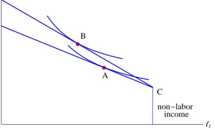
spent on consumption. The optimal choice of how much labor to supply (or leisure to have) depends on the size of real wage and on the size of non-labor income. If an agent is satisfied with the amount of consumption he gets from a non-labor income, then his optimal choice is at point theA as in Fig. 1.

.

non-labor income A

{t C_t

Figure 1: At point theAan agent does not supply labor and consumes to the extent of non-labor income.

The raise in government transfers or in gross nominal interest rate increases income and an agent consumes more with his level of leisure being higher as it can

be observed in Fig. 2.

.

.

Figure 2: Expansion of consumption and leisure due to raise in transfers and/or nominal interest rate.

Now we take into account variations in real wage. The raise in real wage makes the budget line to be steeper by rotation around the point C as Fig. 3 shows. Increase in real wage results in substitution or income effects. With higher real wage leisure becomes more expensive, and an agent substitutes leisure for work, increasing intensiveness of labor, thus, substitution effect takes place. A higher real wage makes an individual richer and he increases consumption and leisure, thus, income effect dominates.

Next we proceed to optimal consumption path. The Euler equation, i.e.intertemporal MRS between consumption in period t and t+ 1 (see Appendix A2):

Uc,t βUc,t+1 =RtEt Pt Pt+1 (3.14)

where 0 < β < 1 is the discount factor (β = 1/(1 + δ), δ > 0 is the rate of time preferences, i.e. the future utility is less valuable than the utility in current period),Rtis gross interest rate, i.e. Rt= (1 +it), that measures the gain (or loss)

.

.

Figure 3: With a higher real wage consumption and labor supply increase (substitution effect).

conditional on information known at timet, and the termEt(Pt/Pt+1) is the inverse

of the gross inflation rate between period t and t+ 1, (1/(1 +πt+1)).

The condition (3.14) is considered to be optimal if a reallocation of consumption between periods t and t+ 1 does not have any influence on the expected utility, while keeping consumption and employment rate unchanged in any other periods, that is:

Uc,tdCt+βEt{Uc,t+1dCt+1}= 0 (3.15)

for any pair (dCt, dCt+1) satisfying:

Pt+1dCt+1 =−PtRtdCt. (3.16)

The latter equation shows that an increase in consumption in periodt+1 is possible only if additional savings invested into one-period bonds in period t take place.

Rearranging terms in equation (3.14) we obtain:

1/Rt=βEt Uc,t+1 Uc,t Pt Pt+1 , (3.17)

and the functional form of the Euler equation reads:

1/Rt=βEt " Ct+1 Ct −ν Xt+1 Xt ν−σ Pt Pt+1 # , σ6=ν. (3.18)

The Euler equation is the key intertemporal condition in general equilibrium mod-els and it determines allocation of consumption over time. It signifies that utility lost from consumption today equals utility from consumption tomorrow adjusted for the gain from keeping bonds. Again, the inequality of intertemporal and in-tratemporal elasticities (ν 6=σ) plays a very important role here. It is responsible for non-separable condition that makes intertemporal consumption dependent on variations in real balances.

For further analysis we need to introduce the budget constraint for periodt+ 1:

Pt+1Ct+1+Rt−1At+2+ (1−R−t1)Mt+1 =At+1+Wt+1Nt+1−Tt+1. (3.19)

At the beginning of period t + 1 an agent receives labor income Wt+1Nt+1 and

taxes/transfers from a government Tt+1. An agent carries over a positive

aggre-gate asset At+1 from period t. After setting the income sources an agent decides

how much to spend on consumption, aggregate assets with gross nominal interest rate and money balances, bearing the opportunity cost of holding money. For convenience of the reader we summarize both budget constraints (3.4) and (3.19):

PtCt+R−t1At+1+ (1−Rt−1)Mt =At+WtNt−Tt (3.20)

Pt+1Ct+1+Rt−1At+2+ (1−R−t1)Mt+1 =At+1+Wt+1Nt+1−Tt+1. (3.21)

The budget constraints have one common variable aggregate assetAt+1 that links

them. Aggregate asset At+1 indirectly shows economic behavior over time and

its dependence on both budget constraints. Combining budget constraints and solving for At+1 in period t+ 1, we obtain:

InsertingAt+1 into period t budget constraint and rearranging terms we have: PtCt+ Pt+1Ct+1 Rt +At+2 R2 t +(1−R −1 t )Mt+1 Rt +(1−R−1 t )Mt=At+WtNt+ Wt+1Nt+1 Rt −Tt− Tt+1 Rt . (3.23) The new budget constraint is a lifetime budget constraint (LBC). The right hand side of LBC represents current and future wealth. The left hand side of LBC rep-resents the distribution of lifetime resources between intertemporal consumption, aggregate assets and money holdings. From the expression above we find Ct+1:

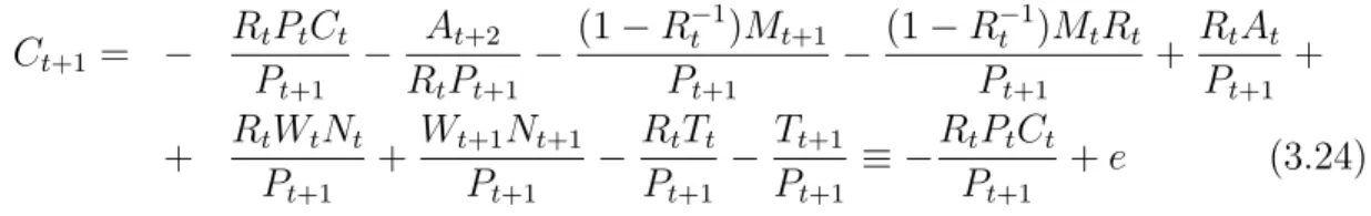
Ct+1= − RtPtCt Pt+1 − At+2 RtPt+1 − (1−R −1 t )Mt+1 Pt+1 − (1−R −1 t )MtRt Pt+1 + RtAt Pt+1 + + RtWtNt Pt+1 +Wt+1Nt+1 Pt+1 −RtTt Pt+1 − Tt+1 Pt+1 ≡ −RtPtCt Pt+1 +e (3.24)

where we define a new variable e for simplicity of notation. We arrived at the budget line with slope (−RtPt

Pt+1), where e is intercept with the vertical line, and Ct = eP_Rtt_P+1_t is the intercept with the horizontal line. Fig. 4 shows an agent’s

optimal consumption choice over time.

.

A

C

Y

C

C

Y

C

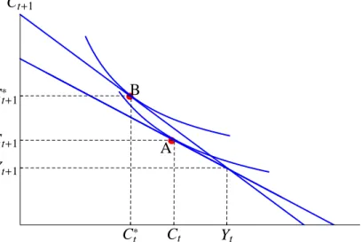
Figure 4: The optimal allocation of consumption over time. Since the representative agent makes savings during periodt, then consumptionCtis less than total incomeYt, and consumptionCt+1

is greater than total incomeYt+1.

interest rate and the ratio of current and future prices. IfPt6=Pt+1, then we have

to deal with inflation over time. The definition of inflation is πt+1 = Pt+1

−Pt

Pt and

the inverse relation is _1+π1

t+1 = Pt

Pt+1, consequently the slope of the budget line is

− 1+it

1+πt+1, according to Fisher relation−

1+it

1+πt+1 =−(1 +rt), thus, the slope of LBC

depends on the real interest rate.

Next we consider how the change of the real interest rate affects the intertem-poral economic behavior. In Fig. 5 we can see that the rise in the real interest rate rotates the budget line around the point (Yt, Yt+1). Increase in the real interest rate

.

.

Figure 5: A rise in the real interest rate increases savings in periodt, by reducing consumption fromCttoCt∗, and extends consumption in periodt+ 1 fromCt+1 toCt+1∗ .

enforces an agent to save, cutting current consumption in order to make profitable investments. Let us take an example to clarify this statement. An agent cuts one unit of consumption in period t, saving some amount of money equivalent to a current price of one unit of consumption Pt. An agent makes an investment with

interest rate it and gets a return in period t+ 1 to the extent of Pt(1 +it), thus,

the profit from investment can buy Pt(1+it)

Pt+1 =

(1+it)

1+πt+1 = 1 +rt units of consumption

consumption an agent can buy in the future.

However, increase in the real interest rate may cause the reverse effect, that is an agent may increase consumption in period t or keep it on the same level. We can see the two effects similar to those in consumption-leisure choice: substitution effect, when an individual reduces current consumption level, or income effect -rise in current consumption.

Finally, we move to the optimal money demand equation, i.e. MRS between real money balances and consumption (see Appendix A3):

Um,t Uc,t = 1−R −1 t = it 1 +it. (3.25)

The money demand equation is considered to be optimal if deviations of consump-tion and money holdings from optimal path do not change the utility, while keeping all other variables constant:

Uc,tdCt+Um,t

1

Pt

dMt= 0 (3.26)

for any pair (dCt, dMt) satisfying:

PtdCt+ (1−R−t1)dMt= 0. (3.27)

Equation (3.27) guarantees that no other variables need to be adjusted in the budget constraint. The functional form is the following:

Mt Pt =Ct(1−exp{−it})− 1 ν ϑ 1−ϑ 1_ν (3.28)

the marginal rate of substitution between money and consumption equals to the opportunity cost of holding money, the relative price between money and con-sumption. Wealth holdings in terms of money balances result in loss of interest income that is paid by alternative assets. Choosing the optimal consumption-money condition, an agent always sets the MRS equal to a function of nominal interest rate.

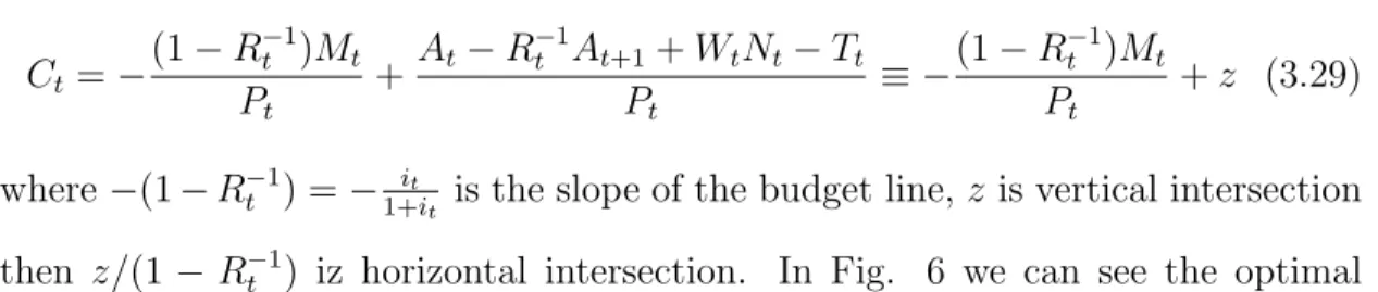
From the budget constraint (3.4) we have: Ct=− (1−R−_t1)Mt Pt + At−R −1 t At+1+WtNt−Tt Pt ≡ −(1−R −1 t )Mt Pt +z (3.29) where−(1−R−_t1) =− it

1+it is the slope of the budget line,z is vertical intersection

then z/(1− R−_t1) iz horizontal intersection. In Fig. 6 we can see the optimal consumption- real balances choice.

.

A

M

Pt

C

Figure 6: Optimal consumption-money choice with the given nominal interest rate.

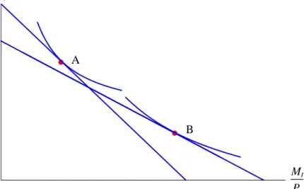
Next we analyze how the variations in nominal interest change the optimal consumption-money choice. If the nominal interest rate increases, the budget line becomes flatter, as in Fig. 7, and decrease in consumption and “increase in real money balances” take place. What is meant by “increase in real money balances” is that an agent does not hold them in cash, instead he invests every extra unit of real money balance into interest bearing assets and gets a return in the next period to the extent of it

1+it. Consequently, when the nominal interest rate goes

up, it is more profitable to keep wealth in terms of less liquid assets and obtain an interest return. In case of interest rate reduction the relative price of holding money decreases and preferences of an agent switch to holding more real balances

and expanding consumption.

.

.

Figure 7: New optimal consumption-money choice after the increase in nominal interest rate.

Optimal labor supply (3.12) and the Euler equation (3.18) depend on the level

of real money balances through the Xt composite index. The optimal money

demand condition (3.28) shows the dependence via the nominal interest rate. Due

to non-separable property of the utility function (σ 6=ν), variations in money level

play an essential role since they determine the equilibrium values of real variables.

3.2

The Firm

We have small representative firm that makes the profit-maximization decision. We assume perfectly competitive markets, and then the firm takes prices in goods and labor markets as given. The firm produces goods according to the following linear production function:

with technology level At and labor level Nt. The level of technology evolves according to a stochastic process, and we log-linearize the technology level so that at ≡ logAt. We assume that production function is strictly increasing

in labor input YN(At, Nt) > 0, and has a diminishing marginal return of labor

YN N(At, Nt)<0.

The firm maximizes its profit subject to the production function (3.30):

PtY(At, Nt)−WtNt. (3.31)

Since the firm is a price taker, it makes the only decision on how much labor to hire. To find the optimal labor demand we take partial derivative with respect to laborNt:

PtYN(At, Nt)−Wt ⇔PtAt−Wt = 0, (3.32)

thus, the marginal product of labor (MPL) is:

YN(At, Nt) =At =

Wt

Pt

. (3.33)

The economic meaning of MPL is how much extra output the firm can produce if it hires an extra unit of labor input, keeping technology level constant. Equality of MPL to the real wage Wt

Pt means that profit maximizing firm hires such number

of labor units so that (real) MPL should exactly equal to the market real wage.

YN(At, Nt) =Wt/Pt is a labor demand function, a relationship between real wage

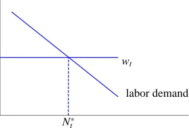
and optimal labor demand that arises due to demand for firm’s output. Earlier we have assumed that the second derivative of the production function is strictly negative YN N(At, Nt)<0, then MPL is decreasing if N increases, that is with an

additional unit of labor input the MPL diminishes (diminishing marginal product of labor). Graphically market real wage is a horizontal line, and the labor demand is a downward-sloping line. The optimal labor demand is the intersection of a labor demand curve and a real wage line as we can see in Fig 8.

labor demand

w

N

N

MPL

Figure 8: Optimal labor demand

Finally, the price of output goods should equal to the marginal cost, and from (3.33) we have: Pt= Wt At . (3.34)

3.3

Log-linear Approximation

The above model contains a nonlinear system of equations which is quite hard to solve. Therefore it is necessary to log-linearize the model around the steady state in order to get a system of linear equations which describe the dynamical behavior of the model for small deviations around the steady state.

Log-linearization of the optimal conditions that characterize the equilibrium of the model is a widely used technique (Uhlig). This method was introduced by King, Plosser and Rebelo (1987), and Campbell (1994) for a basic non-monetary, real-business-cycle model. The approach was extended by Uhlig (1999). Log-linear methods can also be applied to the MIUF model to study dynamics.

The idea of log-linearization is to use Taylor approximation around the steady state. Application of this method allows to replace nonlinear optimal conditions

with linear functions in the log-deviations of the variables and solve the model ana-lytically while still keeping the original interpretations of the variables unchanged.

Formally, letXt be a strictly positive variable and X its steady state. Then

xt ≡logXt−logX

is the log-deviation of a variable from its steady state and it shows how much the variable differs from its steady state value in percentage, Uhlig (1999). In order to incorporate the first-order Taylor approximation into our model we have to define the steady state of the variables, that is Pt = P, Ct = C, Mt = M, Rt = R and

R≡1 +i.

We start log-linearization with the labor supply equation (3.12) that gives us:

wt−pt =σct+ϕnt+ (ν−σ)(ct−xt). (3.35)

Money demand condition (3.28) is complicated by the presence of the unit price of money balances (1−R−_t1 = 1−exp{−it}), so we first need to make a log-linear approximation of that component:

log(1−R_t−1) = log(1−R−1exp{−it})

= log(1−R−1)− 1 1−R−1_exp{−i}(−R −1_exp{−i})(i t−i) = log(1−R−1) + (1−R−1)−1R−1it = log(1−R−1) + (R−1)−1it = (R−1)−1it= 1 exp{i} −1it. (3.36)

Substituting results into the log-linear money demand equation yields:

mt−pt =ct−ηit (3.37)

whereηis the implied interest semi-elasticity of money demand,η = (ν[Rt−1])−1 =

1

and consumption ν−1. One can see the economic interpretation of this equation. If consumption ct is above its steady state, then more money is needed to

sup-port such consumption, which leads to an increase in money demand. On the other hand, a higher nominal interest rateit makes the opportunity cost of hold-ing money higher and money demand goes down since an agent prefers to keep his wealth in interest-earning assets.

Next we make log-linear approximation for the composite index of consumption and real money balancesXt :

Xt≡ " (1−ϑ)C_t1−ν +ϑ Mt Pt 1−ν# 1 1−ν . (3.38)

Then rearranging terms:

X_t1−ν = (1−ϑ)C_t1−ν +ϑ Mt Pt 1−ν (3.39)

and using log-linear approximation r