c
LOGLINEAR MODELS AS ITEM RESPONSE MODELS
BY ZHUSHAN LI
DISSERTATION
Submitted in partial fulfillment of the requirements
for the degree of Doctor of Philosophy in Educational Psychology in the Graduate College of the
University of Illinois at Urbana-Champaign, 2010
Urbana, Illinois
Doctoral Committee:
Professor Carolyn J. Anderson, Chair Professor Hua-hua Chang
Professor Jeffrey A. Douglas
Louis A. Roussos, PhD, Measured Progress Associate Professor Jinming Zhang
Abstract
For analyzing item response data, item response theory (IRT) models treat the discrete responses to the items as driven by underlying continuous latent traits, and consider the form of conditional probability of the response to each item given the latent traits. In a similar fashion, log-linear models directly consider the form of the manifest probability of response patterns. Researchers have been connecting the two paradigms by establishing equivalence relationships between IRT models and log-linear models. This has lead to the notion of obtaining IRT solutions by fitting their equivalent log-linear models.
In this research, I have established a family of log-linear models, log linear-by-linear association (LLLA) models, that incorporate a variety of IRT models, particularly, a family of generalized Rasch models. I have derived an extension of the Dutch Identity theorem to polytomous items and utilized it to develop the models that incorporate item covariates and person covariates. Noteworthy features of the models include both polytomous responses and multiple latent traits.
Along with developing this new family of models, I have conducted extensive research on the development of an accompanying estimation method. Historically, a significant bar-rier to the application of log-linear models in analyzing item responses has been the high computational cost of maximum likelihood estimation (MLE), due to the fact that the num-ber of response patterns grows exponentially as the numnum-ber of items increases. To solve this computational problem, a pseudo-likelihood estimation (PLE) method is proposed and it dramatically decreases the computational cost.
To demonstrate the effectiveness of the developed models and the pseudolikelihood estimation method, I will present results of a series of simulation studies. To demonstrate the practical advantages of the methods, I will give a detailed description of an application to a real data set from a study on verbally aggressive behavior.
Acknowledgments
Completing a doctoral degree has been a fantastic journey for me because of the strong support I received from numerous people over the past years. I am very grateful for the support of families and friends who helped me as I worked on this dissertation. I would like to thank my husband Feng and my daughter Susan for their love. They make my life full, balanced, and happy. My love to them is beyond words I can describe. I would like to thank my parents and my parents-in-law and my siblings in China for their endless encouragement, love and support. I would like to thank the families of Robert and Susan Spellman and their daughters for their tremendous love and support. The love from all my families has been both a trusted guidance and deeply cherished treasure through the years. It is your love that means the world to me.
I am very fortunate to have such a wonderful committee, Carolyn Anderson, Hua-hua Chang, Jeff Douglas, Louis Roussos and Jinming Zhang. They are not only mentors but also friends. I would like to thank my advisor Carolyn who was willing to support me and share her personal stories and advice with me. Her trust and encouragement of my doing good research has given me a lot of confidence. I really appreciate her for encouraging me to think independently. I deeply appreciate my early research advisor and mentor Louis Roussos for his leading me into the field and providing a good foundation for my research. His kindness, love, passion, and willingness to help students deeply influenced me and set a very good model for my future career. I am very grateful to Professor Jeff Douglas for supporting me financially to go to the AERA and NCME conferences. Your wonderful teaching, rich knowledge, useful suggestions, kindness, and support for my research will be remembered forever. Professor Hua-hua Chang’s comments on my solid knowledge foundation, good communications skills, and very strong research encouraged me and motivated me to do a better job and helped me to achieve better. His support for my work deeply touched me
and I deeply appreciate his encouragement. Professor Jinming Zhang is a very bright and nice person and gave me many good suggestions.
I want to thank the Department of Educational Psychology and the Department of Statistics for providing financial aid through my doctoral studies. I also want to thank various award committees for giving me awards for my research, which encouraged me to do better and achieve better. The secretaries in our department have been very supportive all these years. I want to thank all of you, especially my friends Helen and Julie who have been there for me many times.
My training in the Department of Statistics will benefit me forever. I deeply ap-preciate many professors there. In particular, John Marden, John Martinsek, Jeff Douglas, Xuming He, Xiaofeng Shao, Feng Liang, Barbara, Doug Simpson, and Ombao supported me in different ways.
Many friends helped and supported me during my time at University of Illinois. Peter Cao and Amy Li provided their home and food for us on many occasions. Their friendship is more like another family. Ann and Russell helped us a lot when we were in need. My friend Sherman always believed in me and trusted me in doing good research. My friends Cha-chi, Charles, Hongling, Xiangkui, Haiyan, Yiming, Rongchun, EunYoung, Holly Downs, Xiaolin, Xiaofang, Jianxin, Yinping, Min Li, Shiqiu, Shenfang, Shuqing and Peilin provided a lot of support and help. While I am thinking about all my friends, I cannot list all of them here, I feel very blessed to have had such an amazing group of friends during my years at UIUC. My friends Bill and Kathryn Scott and the home group in Rantoul supported us tremendously. I also want to thank Calvary Campus Church, Stone Creek Church and Christian Life Church and CBS friends. I also want to thank all my friends in BCBSG fellowship. Your prayers and love for me has been my strength all these years.
Finally, I would like to give thanks to God for his grace and blessings in my life. May His glory shine through my life.
Table of Contents
List of Tables . . . ix
List of Figures . . . xi
List of Abbreviations . . . xiii
List of Symbols . . . xiv
Chapter 1 Introduction . . . 1
Item Response Theory Models . . . 1
Log-linear Models . . . 3
Connecting Two Paradigms . . . 6
Research Objectives . . . 7
Adding covariates . . . 9
Polytomous and multidimensional models . . . 11
Summary . . . 12
Chapter 2 LLLA as IRT Models . . . 14
Assumptions for LLLA model . . . 14
LLLA Model as Rasch Model . . . 17
Dutch Identity . . . 20
Fitting Rasch by LLLA . . . 24
Item parameters . . . 24
Person parameters . . . 24
Population latent trait distribution . . . 27
Mixture of conditional normals: demonstrations by simulated data . . . 29
Chapter 3 Pseudolikelihood Estimation . . . 34
MLE for LLLA Model . . . 35
Motivation of PLE for LLLA . . . 37
Introduction to PLE . . . 39
Application of PLE to LLLA . . . 40
Maximize PL Using Logistic Regression . . . 44
Correct Standard Errors . . . 46
Jackknife . . . 46
Bootstrap . . . 47
Chapter 4 LLLA With Covariates . . . 50
IRT Models With Covariates . . . 51
Item covariates . . . 51
Person covariates . . . 51
LLLA With Item Covariates . . . 52
LLLA With Person Covariates . . . 53
Model form . . . 54
Derivation of LLLA with person covariates model . . . 54
Connection and difference with latent regression Rasch model . . . 56
Chapter 5 Polytomous Models . . . 58
Review of Polytomous IRT Models . . . 59
Definition of polytomous logit functions . . . 60
Three classes of polytomous IRT models . . . 64
The family of partial credit models . . . 64
Dutch Identity for Polytomous Models . . . 66
Derivation of the LLLA Model From Bock’s Model and the PCM . . . 69
Polytomous Models With Item Covariates . . . 71
Partial credit model with item covariates . . . 71
LLLA model with item covariates . . . 72
Polytomous Models With Person Covariates . . . 74
Partial credit model with person covariates . . . 74
LLLA model with person covariates . . . 75
Chapter 6 Multidimensional Models . . . 77
Multidimensional LLLA Model . . . 78
Dichotomous model . . . 78
Polytomous model . . . 82
Estimating Rasch parameters . . . 90
Multidimensional LLLA Model With Item Covariates . . . 93
Dichotomous model . . . 93
Polytomous model . . . 96
Estimating Rasch parameters . . . 100
Multidimensional LLLA Model With Person Covariates . . . 102
Dichotomous model . . . 102
Polytomous model . . . 106
Estimating Rasch parameters . . . 110
Chapter 7 Simulation Studies . . . 116
Unidimensional Dichotomous Models . . . 119
LLLA with item covariates . . . 119
LLLA with person covariates . . . 123
Unidimensional Polytomous Models . . . 132
Polytomous LLLA with item covariates . . . 132
Multidimensional Dichotomous Models . . . 143
Multidimensional LLLA with Item covariates . . . 143
Multidimensional LLLA with person covariates . . . 146
Multidimensional Polytomous Models . . . 151
Multidimensional polytomous LLLA with item covariates . . . 151
Multidimensional polytomous LLLA with person covariates . . . 154
Chapter 8 Real Data Analysis . . . 159
Computation Time . . . 161
Rasch Model . . . 161
LLTM . . . 164
Latent Regression Rasch Model . . . 168
Partial Credit Model . . . 169
Partial Credit Model With Item Covariates . . . 172
Partial Credit Model With Person Covariates . . . 173
Chapter 9 Conclusion . . . 178
Flexibility of the Models . . . 178
Flexibility on Latent Trait Distribution . . . 179
Pseudolikelihood is Fast . . . 180
Non-collapsibility of LLLA Models . . . 181
Interpretation of the LLLA Parameters . . . 181
Differential Item Functioning . . . 182
Estimation for IRT 2PL Model and Bock’s Model . . . 182
List of Tables
1 An Example of a Data Matrix From a 4-item Binary Test . . . 1
2 Different Formulations of the Rasch Model . . . 19
3 Original Response Data Matrix . . . 36
4 Response Data in Count Data Format . . . 37
5 Design Matrix for the LLLA Model . . . 38
6 Stacked Data in Pseudolikelihood Estimation With Logistic Regression Procedures . . . 45
7 Simulation Designs . . . 117
8 MLE and PLE Obtained From Fitting the LLLAi Model on Simulated Data With 5 and 10 Items . . . 120
9 Comparing the Robust Estimates (“Sandwich” Estimator) of the SE’s to True SE’s for the LLLAi models by Monte Carlo Simulation. Each Model was Replicated 10,000 Times . . . 123
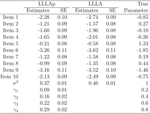
10 Parameter Estimates of the LLLAp Model and the LLLA Model Along With the True Parameters for the 10-item Test . . . 127
11 Comparing the Robust Estimates (“Sandwich” Estimator) of the SE’s to True SE’s for the LLLAp models by Monte Carlo Simulation. Each Model was Replicated 10,000 Times. For the Tests With Length 10, 50 and 100 Items, the Item Effects for Only the First 5 Items . . . 131
12 MLE and PLE Obtained From Fitting the LLLAi Model on Simulated (Polytomous) Data With 5 and 10 Items . . . 134
13 Parameter Estimates of the LLLAp Model and the LLLA Model Along With the True Parameters for the 10-item (Poly-tomous) Test . . . 140
14 MLE and PLE Obtained From Fitting the LLLAi 2D Model on Simulated (Polytomous) Data. Test Length I = 6 and 10 Items . . . 145
15 MLE and PLE Obtained From Fitting the LLLAi (2D) Model on Simulated Data. Test Length I = 10 Items. Polytomous items With 3 Categories . . . 153
16 IRT Models for the Real Data Set . . . 159
17 Time Cost of Fitting IRT Models on Verbal Aggeression Data . . . 162
18 Parameter Estimates and Standard Errors for the Rasch Model (Verbal Aggression Data) . . . 163
19 Parameter Estimates and Standard Errors for the LLTM (Ver-bal Aggression Data) . . . 166
20 Parameter Estimates and Standard Errors for the Latent Re-gression Rasch Model (Verbal AgRe-gression Data) . . . 169
21 Parameter Estimates and Standard Errors for the Partial Credit Model (Verbal Aggression Data) . . . 171
22 Parameter Estimates and Standard Errors for the Partial Credit
Model With Item Covariates (Verbal Aggression Data) . . . 174 23 Parameter Estimates and Standard Errors for Partial Credit
Model With Person Covariates (Verbal Aggression Data) . . . 175 24 Models That can be Fit by R Package ‘plRasch’ . . . 179
List of Figures
1 Rasch model’s item response function. . . 3
2 Contingency table for a 2-item test with dichotomous responses . . . 4
3 Extended Rasch models. . . 8
4 Research strategies. . . 11
5 Graphical structure of the 1-D LLLA model. . . 15
6 Population latent trait distributions, standard normal, 10 items. . . 29
7 Population latent trait distributions, two-component mixture of normal, 10 items. . . 31
8 Population latent trait distributions, two-component mixture of normal, 50 items. . . 32
9 Baseline category logits. . . 61
10 Adjacent category logits. . . 62
11 Cumulative logits. . . 63
12 Sequential logits. . . 63
13 PLE vs MLE for item covariates effects. Test length I = 5 and 10 items. . . 121
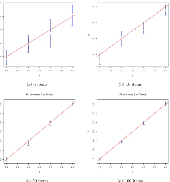
14 PLE vs true item covariate effects. Test lengthI = 5, 10, 50, and 100 items. . . 122
15 PLE vs true person covariate effects. Test length I = 5, 10, 50, and 100 items. . . 126
16 Parameter estimates and SEs for λ by the LLLAp and LLLA models. . . 128
17 Three-way comparison of the true, LLLAp estimated, and LLLA estimated item difficulty parameters βi. . . 129
18 Three-way comparison of the true, LLLAp estimated, and LLLA estimated person ability parametersθp. . . 130
19 PLE vs MLE for item covariates effects. Test length I = 5 and 10 items. . . 133
20 PLE vs true item covariate effects. Test lengthI = 5, 10, 50, and 100 (polytomous) items. . . 136
21 PLE vs true person covariate effects. Test length I = 5, 10, 50, and 100 items. . . 138
22 Parameter estimates and SEs for λ by the LLLAp and LLLA models. . . 139
23 Three-way comparison of the true, LLLAp estimated, and LLLA estimated item difficulty parameters βi(h). . . 141
24 Three-way comparison of the true, LLLAp estimated, and LLLA estimated person ability parametersθp. . . 142
25 PLE vs MLE for item covariate effects. 2-D latent traits, Test lengthI = 6 and 10 items. . . 146
26 PLE vs true item covariate effects. Test lengthI = 6, 10, 50, and 100 items. 2-D latent traits and dichotomous response. . . 147
27 PLE vs true person covariate effects. Test length I = 6, 10,
50, and 100 items; 2-D latent traits and dichotomous responses. . . 149 28 Fitted person covariates vs true parameters with “unbalanced”
item loadings. Test lengthI = 50 and 100 items. . . 151 29 PLE vs MLE for item covariate effects. Test lengthI = 6 and
10 items; 2-dimensional latent traits, 3 category responses. . . 154 30 PLE vs true item covariate effects. Test lengthI = 6, 10, 50,
and 100 items, 2-dimensional latent traits, 3 category response. . . 155 31 PLE vs true person covariate effects. Test length I = 6, 10,
50, and 100 items; 2 dimensional traits, 3-category responses. . . 158 32 Item difficulty estimates for the Rasch model, LLLA (PL) vs
GLMM (NLMIXED). . . 164 33 Item covariate effects estimates for the LLTM, LLLA (PL) vs
GLMM (NLMIXED). . . 166 34 Person covariate effects estimates for the latent regression Rasch
model, LLLA (PL) vs GLMM (NLMIXED). . . 170 35 Item difficulty estimates for the partial credit model, LLLA
(PL) vs GLMM (NLMIXED). . . 172 36 Item covariate effects estimates for the partial credit model
with item covariates, LLLA (PL) vs GLMM (NLMIXED). . . 175 37 Person covariate effects estimates for the partial credit model
List of Abbreviations
CML Conditional maximum likelihood
GLMM Generalized linear/nonlinear mixed models ICRF Item category response function
IRF Item response function IRT Item response theory
LLLA Log linear-by-linear association model
LLLAi Log linear-by-linear association model with item covariates LLLAp Log linear-by-linear association model with person covariates LLTM Linear logistic test model
LMA Log multiplicative association model MLE Maximum likelihood estimation MML Marginal maximum likelihood PCM Partial credit model
PCMi Partial credit model with item covariates PCMp Partial credit model with person covariates PLE Pseudolikelihood estimation
List of Symbols
Θ, θ latent traits Y, y responses X, x item covariates
Z, z person covariates
a item discrimination; entries in item-trait adjacency matrix b item parameter
β item covariate effect γ person covariate effect σ2 variance
σ2
0 variance conditional on response pattern
λ intercept in the LLLA model
λi(yi) item parameter forith item with response yi in the LLLA model νi(yi) score forith item with response yi in the LLLA model
Σ variance-covariance matrix
σdd0 entries in the variance-covariance matrix T, t total score
p subscript for pth person i subscript for ith item
h subscript for hth response category k subscript for kth item/person covariate d subscript for dth latent trait
N number of persons (examinees) in the test I number of items in the test
m the highest response category D number of latent traits
Chapter 1
Introduction
The general purpose of my research is to model item response data in a log-linear model framework. Item response data are generated when people give responses to items in a battery where the goal is to measure some underlying latent trait or ability. Suppose there are N examinees who respond to I items. Let Ypi be the coded response of the pth person
to the ith item. Very often the response is dichotomous, and Ypi is coded as 1 (=correct)
and 0 (=incorrect). The observed item responses of a person Yp = (Yp1, . . . , YpI) are used
to evaluate the person’s ability that is assumed to be a continuous latent variable Θ. Table 1 is an example of a data matrix from a 4-item binary test with 1000 examinees (N = 1000 andI = 4). The data matrix is a 1000 by 4 with 0-1 entries. Each row represents a person’s response to the test items, and each column represents an item responded by all the persons.
Table 1
An Example of a Data Matrix From a 4-item Binary Test
Person Item 1 Item 2 Item 3 Item 4
1 0 1 0 1 2 1 0 1 0 3 1 1 1 1 4 0 1 1 1 ... ... ... ... ... 1000 1 0 0 0
Item Response Theory Models
Item Response Theory (IRT) models have been developed to model the structure of the relationship between the manifest (observed) item responses and latent traits (Lord & Novick, 1968; Lord, 1980; Baker & Kim, 2004; Hambleton, Rogers, & Swaminathan, 1995;
Van der Linden & Hambleton, 1997; Embretson & Reise, 2000; Boomsma, Duijn, & Snijders, 2001). A central assumption in IRT models is local independence; that is, given the latent traits, the responses to items are independent of each other. Specifically, local independence implies that the joint distribution of responses to a set of items can be expressed as the product of the probability of each individual response conditional on the latent trait; that is, p(yp|θp) = P(Yp1 =yp1, Yp2 =yp2, . . . , YpI =ypI|Θp =θp) = I Y i=1 P(Ypi =ypi|Θ = θp) = I Y i=1 p(ypi|θp), (1.1)
where P(Ypi = ypi|Θ = θp) is the conditional probability that a person with latent trait
θp gives one specific response ypi to item i, and p(yp|θp) is the conditional probability that
personpwith latent traitθp gives response patternyp to all items. With local independence,
we only need to model the conditional probability of responses to each item given the latent trait.
For dichotomous items with coded values of 0 or 1,Ypifollows a Bernoulli distribution.
LetPi(θp) =P(Ypi = 1|θp) and Qi(θ) =P(Ypi= 0|θp) = 1−Pi(θ), then
p(ypi|θp) =Pi(θp)ypiQi(θp)1−ypi.
The term Pi(θp) that represents a function of the latent trait is called an item response
function (IRF).
The Rasch model (Rasch, 1960, 1961) is the simplest yet a very important IRT model. For a description and discussion of recent developments in the Rasch model and related models including the models with covariates that I am going to discuss in this thesis, see Fischer and Molenaar (1995), De Boeck and Wilson (2004), and von Davier and Carstensen
(2007). The Rasch model specifies the IRF for responses to dichotomous items with a single latent trait. The IRF for the Rasch model is given by
Pi(θp) =P(Ypi= 1|θp) =
exp(θp −bi)
1 + exp(θp−bi)
, (1.2)
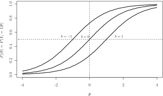
where bi is the difficulty parameter of the ith item. Figure 1 shows the Rasch IRF curves
for three items with difficulty b=−1, 0, and 1.
-4 -2 0 2 4 0. 0 0. 2 0. 4 0. 6 0. 8 1. 0 θ Pi ( θ ) = P ( Yi = 1 | θ ) b=−1 b= 0 b= 1
Figure 1. Rasch model’s item response function.
The form of the Rasch model reflects the fact that the probability of the response to an item depends not only on the latent trait of the person who answers the item (person parameter θp), but it also depends on the characteristics of the item itself (i.e, the difficulty
of the item that is represented by the item parameter bi).
Log-linear Models
Another broad family of statistical models for analyzing discrete response variables is log-linear models (Agresti, 2002). Log-linear or Poisson regression models are regressions for count data that may be entries in a cross-classification by two or more variables. The
dependency structure between the variables is modeled by the linear model that contains, for example, marginal effects, two-way interactions, and three or higher-way interactions. The paradigm of log-linear models has been well developed and is a standard statistical tool for multivariate categorical data analysis.
Item response data can be expressed as cross classifications by items. To see this, consider a simple example of a test with only two items and 1000 examinees (Figure 2). The response data are represented by a 1000×2 matrix and the entries in the matrix are the observed 0-1 responses (Figure 2 (a)). The same data can be represented by a 2×2 contingency table (as shown in Figure 2 (b)), with rows representing the outcomes for the first item and columns for the second item, and the entries in the four cells of the contingency table are the count of persons with each of the response patterns. In this example, there are 100, 200, 300, and 400 persons with the response pattern (0, 0), (0, 1), (1, 0), and (1, 1), respectively. The contingency table is often represented in a “long” form (as shown in Figure 2 (c)), where all the response patterns are listed row by row in a data matrix, and a column of counts is attached to the data matrix. Such “long” form representation is often used for multi-way contingency tables beyond 3-way table.
person item1 item2
1 0 1
2 1 0
3 1 1
... ... ...
1000 1 0
(a) data matrix
item2
item1 0 1
0 100 200 1 300 400
(b) 2x2 table
item1 item2 count
0 0 100
1 0 300
0 1 200
1 1 400
(c) long form
Figure 2. Contingency table for a 2-item test with dichotomous responses
In general, for item response data the response to each item is a discrete random variable and responses to all the items can be considered as entries in a multi-way table such that each cell in the table represents a response pattern for a set of items. The cell probability is the probability that a randomly selected person gives response pattern (Y1, . . . , YI), where
each variable corresponds to a response to an item. The probabilities of response patterns denoted byP(Y1, . . . , YI) are called manifest probabilities. In the previous 4-item binary test
example shown in Table 1, there are a total of 24 = 16 response patterns (0000, 1000, 0100,
. . ., 1111), and each person’s actual response to the exam falls into one of the 16 patterns. The data can be considered as a 2×2×2×2 or four-way table where each dimension of the table represents a dichotomous item in the test. The observed number of persons answering each pattern forms the count data in the table, and the count data can be analyzed using a log-linear model.
Anderson and Vermunt (2000) proposed log multiplicative association (LMA) models for discrete response data that are derived from a latent variable model. For item response data with a unidimensional latent trait, the LMA model has the form
logp(y) = λ+X i λi(yi)+σ 2X i X i0>i νi(yi)νi0(yi0), (1.3)
where λ is the intercept that ensures that the sum of probabilities over all patterns is 1. The termsλi(yi), i= 1, . . . , I, are the marginal effects of the items, and in a later section we will see they are related to the difficulty of each item. The parameters νi(yi), i = 1, . . . , I, are the scores for each item that are related to item discrimination. The term σ2 is a scale
parameter and equals the variance of the latent variable within a response pattern.
The difference between log-linear and item response models is evident by comparing the LMA model for unidimensional and dichotomous items, as given by (1.3), with the Rasch model, as given by (1.1) and (1.2). Although both the LMA model and the Rasch model describe the same underlying structure, log-linear models are expressed in the form of the manifest probabilitiesp(y), and they do not explicitly include latent traits in the equation. On the other hand, IRT models are expressed as functions of latent variables, and in the form of the conditional probability p(y|θ).
relationship between the manifest probability and the conditional probability. Integrating over the latent trait θ in the joint distribution of manifest variables and latent variables yields the manifest probabilities,
p(y) =
Z
p(y|θ)p(θ)dθ ,
where p(θ) is the distribution of the latent trait in the population. Note that both the conditional probability p(y|θ) and the latent trait distribution p(θ) have to be specified in order to get the manifest probabilities.
Connecting Two Paradigms
Since item response data can be analyzed by IRT models and by log-linear models, people have been interested in the relationship between the two approaches. Cressie and Holland (1983) showed that under certain assumptions, the manifest probabilities of the dichotomous item responses that follow a Rasch model will also follow a log-linear model with second order interactions. Holland (1990) further extends the results into what is called the Dutch Identity theorem that provides a general tool to establish the equivalence between the IRT models for dichotomous items and log-linear models under certain con-ditions. Anderson and Vermunt (2000) proposed the log multiplicative association (LMA) models for the discrete response data that are derived from a statistical graphical model for observed discrete and continuous latent variables. Anderson and Yu (2007) showed that the LMA model is in fact equivalent to the Rasch and the IRT 2-parameter logistic (2PL) models. The equivalence between the IRT models and log-linear models has implications for modeling item response data. It provides a new perspective for fitting the IRT models and opens the doors for new tools for analyzing item response data. Since IRT models have been proven to be useful and have wide applications in educational testing and health outcome research, this provides broad application of log-linear models such as LMA or Log-linear by
linear Association Models (LLLA) in these fields.
Although log-linear models as item response models provide vast potentials for the analysis of item response data, computational problems have to be addressed before the log-linear models can be widely used for most applications. The computational cost of maximum likelihood estimation (MLE) of log-linear models is proportional to the number of cells in the multi-way table. As the number of items in the test increases, the total number of responses increases exponentially, and as a result fitting log-linear models soon becomes infeasible. The MLE procedure described in Anderson and Vermunt (2000) as implemented in the statistical package
`
EM (Vermunt, 1997) cannot be used to fit data sets beyond 12dichotomous items within a reasonable time or amount of memory. An achievement test may have more than 50 and even a hundred items, so the MLE procedures used by
`
EM and other programs will not work for moderate to large problems. To solve the computational cost problem, a pseudolikelihood estimation (PLE) approach was discussed for Rasch models by Strauss (1992), Zwinderman (1995), Smit and Kelderman (2000), and Anderson, Li, and Vermunt (2007). Only the method described in Anderson, Li, and Vermunt (2007) can handle polytomous or binary items and single or multiple latent traits. I implemented the PLE procedure in R and published the R package ‘plRasch’ (cran.r-project.org) . Thepaper describing the first version of the R package ‘plRasch’ was published in the Journal of Statistical Software (Anderson, Li, & Vermunt, 2007). We found that the pseudolikelihood approach is computationally efficient, recovers parameters extremely well, and can be used for large number of items (e.g., 100 items).
Research Objectives
Given the success of PLE for models in the Rasch family, my thesis research objective is to extend my previous work on log-linear models for item response data, and implement the PLE procedures in a software package that can be used to analyze item response data with covariates. My strategy is to start with IRT models with covariates (De Boeck & Wilson,
2004), from which I derive the form of the corresponding log-linear model by utilizing the relationship between the IRT models and log-linear models through the Dutch Identity theorem. I will use pseudolikelihood estimation to estimate the parameters in the derived log-linear models. This would solve the estimation problems for large data sets.
P
(
Y
i
= 1
|
θ
) =
1+exp(
exp(
θ
−
θ
−
bi
bi
)
)
Polytomous IRT Y = 0,1,2, . . . , m Multidimentional IRT Θ = (θ1, θ2, . . . , θD) Person covariates θ=Zγ+ Item covariates bi=Xβ 2PL model ai(θ−bi)Rasch model
1Figure 3. Extended Rasch models.
Many IRT models can be seen as extensions of the Rasch model by modifying different features in the Rasch IRF (Figure 3). For example, the two-parameter logistic (2PL) model (Birnbaum, 1968) adds another item parameter (ai) for each item to represent discrimination
power that differs across items. By including covariates related to item properties and person properties, the IRT models increases their explanatory power. Well-known examples are the linear logistic test model (LLTM) (Fischer, 1973), and the latent regression Rasch model (Zwinderman, 1991). Polytomous IRT models (Ostini & Nering, 2006; Nering & Ostini, 2010) study items that have multiple response outcomes that is often seen in applications. Some well-known polytomous models are Masters’ partial credit model (Masters, 1982), Bock’s nominal response model (Bock, 1972), Samejima’s graded response model (Samejima,
1970), and the rating scale model (Muraki, 1990). When a single latent variable is not enough to explain the all the dependency in the items so that unidimensional local independence is violated, multidimensional IRT models (Reckase, 2009) that assume multiple latent traits may be necessary.
The richness of the family of IRT models is a motivation to draw parallel extensions on the log-linear models for item response data. In the following sections, I will lay out the research objectives of this thesis that include: adding person and item covariates, extending to polytomous items, and to multi-dimensional models.
Adding covariates. With respect to covariates, I intend to extend the log-linear models for item response data to include covariates that are attributes of items and persons. Although the Dutch Identity exists for dichotomous items, I will present an extension so that I can extend log-linear models to polytomous items and multiple latent traits.
Starting with a simple unidimensional dichotomous model, I will show how to add covariates to the model. Item covariates describe the properties of items, such as item type, behavior mode, situation type, and others. Person covariates describe characteristics or attributes of examinees, such as gender, social economic status (SES), ethnicity, and others. In IRT models, the linear logistic test model (LLTM) (Fischer, 1973) was proposed as an extension of the Rasch model that incorporates item covariates, and the latent regression model extends the Rasch model by adding person covariates. Furthermore, models with both item and person covariates have also been proposed. The IRT models that incorporate person and item interactions can be used to model differential item functioning (DIF) (Holland & Wainer, 1993), which is an important research topic on the fairness of test design.
Given the fact that log-linear models are Poisson regression models, it seems that adding covariates is straightforward; however, the log-linear models that I study in this thesis are used as IRT models. The models have a specific structure rather than unrestricted Poisson regression models. Specifically, I will add covariates to the log-linear models with
second order interactions. Since the models will be used as IRT models, the effects of the covariates would retain their interpretation as specified in IRT models.
In the literature there have been efforts in adding covariates to log-linear models with second order interactions. Joe and Liu (1996) proposed a model for multivariate binary response data with covariates. Although Joe and Liu (1996)’s proposal was not IRT based, their model is the same as an LLLA model with person covariates. They specified the model based on compatible conditionally specified logistic regressions. They started with logistic regressions for each variable conditional on other variables and covariates. They derived the conditions to ensure that the set of logistic models were compatible or consistent with some joint distribution, and the joint distribution was shown to be an LLLA model. This conditional specification approach is very closely related to the pseudolikelihood estimation procedure that is described in Anderson, Li, and Vermunt (2007). Conditionally specified logistic regressions can also be used as a tool to derive LLLA models from IRT methodology, as shown in Anderson and Yu (2007), Anderson, Li, and Vermunt (2007), and Anderson, Verkuilen, and Peyton (2010). In Anderson and Vermunt (2000), there is an example of a person variable (i.e., gender) being incorporated into the LMA model using the graphical model approach. In Anderson and B¨ockenholt (2000), an LMA model with covariates was proposed and illustrated by analyzing SES × program type as a function of student mean achievement test scores. In Tettegah and Anderson (2007), an LLLA model with continuous person covariates was used for binary response data. In Anderson et al. (2010), responses of four polytomous items are analyzed where treatment conditions and item content information are used as item covariates.
What I am proposing in this thesis is a systematic way of developing the log-linear models with covariates starting with IRT models with covariates. The approach I will use (the solid lines in Figure 4) is different from the conditionally specified approach (the dotted lines in Figure 4) used in Joe and Liu (1996); Anderson, Li and Vermunt (2007); Anderson and Yu (2007); and Anderson et al. (2010). Instead of starting with a set of logistic
Rasch / 2PL Model Conditonal Normality+ p(yi|θ) p(θ|(0,0, . . . ,0))∼N(µ0, σ20) LLLA / LMA p(y1, y2, . . . , yI)
Logistic Regression / Multinomial Logit
p(y1|y2, y3, . . . , yI)
p(y2|y1, y3, . . . , yI)
p(yI|y1, y2, . . . , yI−1) Dutch Identity
Pseudolikelihood Estimation Conditially Specified Models
replaceθwith rest score
˜
θ=Pj6=iνj
Homogeneous Conditional Gaussian
θ|y1, ..., yI∼N(µy, σ20)
Linear expansion of scores
µy=ν1(y1)+. . .+νI(yi)
Anderson & Vermunt (2000)
Graphical Models
Write down models according to some rules
1
Figure 4. Research strategies.
regressions of each response conditional on other responses and covariates, I start with IRT models with each response conditional on the latent trait and covariates. The advantage of starting directly with IRT models is that the parameters in the models will have a clear interpretation as described in corresponding item response theory models. Furthermore, the pseudolikelihood method provides a computationally efficient way to estimate the parameters and can be used in practical problems.
Polytomous and multidimensional models. I will extend the Dutch Identity theorem to polytomous items and use the polytomous Dutch Identity theorem to derive log-linear models that can be used for ordinal response items that are equivalent to polytomous IRT models such as the partial credit model. In this thesis, I will elaborate how to derive the log-linear models from polytomous IRT models, and develop the log-linear models with covariates that can handle polytomous items.
IRT models with multidimensional latent traits have been an active research area (Ackerman, 1994; Kelderman & Rijkes, 1994; Reckase, 1997a, 1997b, 2009). Log-linear
models estimated by pseudolikelihood methods have a clear advantage in computational feasibility relative to the IRT models estimated by a traditional marginal maximum likeli-hood (MML) approach. In MML, the latent traits have to be numerically integrated out, assuming multivariate normality or some other distribution for the latent traits. Therefore if the number of the latent traits is large, the computational cost of the numerical integration increases exponentially. The log-linear model approach proposed in my thesis does not suffer this kind of problem because no numerical integration is involved in this method.
Summary. To summarize, the following is what is accomplished in this thesis: the development of log-linear models for item response data that incorporate item and person covariates, with the ability to handle both polytomous items and multidimensional latent traits; the complete presentation, from proof to interpretation of the relationship between log-linear models and the corresponding IRT models; and the development and implementa-tion of computaimplementa-tionally efficient estimaimplementa-tion procedures using the pseudolikelihood approach. The remainder of this thesis is structured as follows. In Chapter 2, I will lay out the theoretical basis for this thesis research. I will give an introduction to the LLLA model and show how it can be seen as a equivalent form of the Rasch model. I will introduce the Dutch Identity theorem that is an important tool to prove the equivalence of the log-linear models and the IRT models, and for developing the models in this thesis. In Chapter 3, pseudolikelihood estimation is introduced and I will show how it is applied to the LLLA model. In Chapter 4, I will present the development of LLLA models with item covariates and with person covariates. In Chapter 5, I will present and prove the Dutch Identity theorem for polytomous items and use it to develop polytomous LLLA models that are equivalent to polytomous IRT models, including those with item covariates and person covariates. In Chapter 6, I will derive the LLLA models equivalent to the multidimensional IRT models, including those with item and person covariates. In Chapter 7, simulation studies for all the models developed in this thesis are presented. Chapter 8 contains applications of the
models to a real data set. Finally, the thesis ends with Chapter 9 with a summary and some concluding remarks.
Chapter 2
LLLA as IRT Models
In this chapter, I am going to introduce the equivalence between LLLA models and IRT Rasch models. First I will present the set of assumptions that lead to an LLLA model as presented in the original LMA/LLLA paper (Anderson & Vermunt, 2000). Next I will present another set of assumptions starting with a Rasch model that lead to exact the same LLLA model; thus the LLLA model can be seen as a special form of the Rasch model. Then I will present the Dutch Identity theorem. This theorem is used to derive the LLLA model from the Rasch model. It will be used as the tool to develop the LLLA models with covariates throughout my thesis research. Finally I will show how to estimate the item and person parameters in the Rasch model by fitting the LLLA model.
Assumptions for LLLA model
For a test with I items, the responses of an examinee to the items is a realization of a random vector Y = (Y1, Y2, . . . , YI). The value of the random vector is one of the
QI
i=1ni possible response patterns, where ni is the number of possible response options for
item i. If all the items are binary, then there are 2I possible response patterns. Denote
p(y) =P(Y =y), as the manifest probability for response pattern y. Note that
X
all y
p(y) = 1.
The dependence structure of multiple variables can often be represented by a graph, an integral tool in graphical models (Whittaker, 1990). Consider the case with a single latent trait. The dependency among the variables, including the discrete manifest variables Y1, . . . , YIand the continuous latent trait variable Θ, is reflected in the graph shown in Figure
latent variables are represented by circles; the possible dependence between the variables is represented by lines and paths connecting the variables; and conditional independence is represented by the absence of lines or paths connecting variables.
The concept of local independence is represented in graphical models. As we can see in Figure 5, all the manifest variables Yi may be dependent on the latent trait variable Θ,
as is seen by the edges connecting the manifest variables to the latent variable. Associations among manifest variables are expected to be observed because there are paths connecting the manifest variables through the random latent variable Θ. Since there is no direct edge between any pair of the manifest variables, the manifest variables are independent of each other conditional on the latent trait.
Y
1Y
2Y
3Y
4θ
ν
1(y1)σ
2ν
1(y1)ν
2(y2)ν
1(y1)ν
3(y3)ν
4(y4)Figure 5. Graphical structure of the 1-D LLLA model.
Anderson and Vermunt (2000) derived the LMA models (of which LLLA models are special cases) for the structure represented in Figure 5 by assuming that:
• The observed variables given the latent traits are conditionally independent, (i.e., local independence): p(y|θ) =P(Y =y|Θ=θ) = I Y i=1 p(yi|θ).
• The joint distribution of the discrete variables Y1, . . . , YI and continuous variable Θ
is a homogeneous conditional Gaussian (Lauritzen & Wermuth, 1989). A homoge-neous conditional Gaussian distribution assumes that the conditional distribution of the continuous variable given the discrete variable is normal with constant variance:
Θ|Y =y∼N(µy,Σ).
• The mean of the conditional Gaussian distribution is set equal to a linear expansion of scores: µy =σ2 I X i=1 νi(yi)
In the case of the model with a unidimensional latent trait, the conditional distri-bution of the latent trait is a univariate normal distridistri-bution θ|y ∼ N(µy, σ2). Under this
assumption, Anderson and Vermunt (2000) show that the log manifest probability is given by logp(y) = λ+X i λi(yi)+σ 2X i X i0>i νi(yi)νi0(yi0). (2.1) Model (2.1) is called a log multiplicative association (LMA) model if we assume the scores for each item νi(yi) are unknown and need to be estimated. It is a nonlinear model because of the multiplicative terms σ2ν
i(yi)νi0(yi0). If we assign the scores νi(yi) for each item so they are fixed numbers,1 then (2.1) is a linear model because the right-hand side of the
equation is a linear function of the unknown parameters (i.e., λ, λi(yi), and σ
2), and the
model is called a log linear-by-linear association (LLLA) model (Agresti, 2002).
The distribution p(θ|y) is the posterior distribution of the latent trait given the
1For the assignment of the scores, one popular way is to use the natural score: ν
i(yi)=yi. For example,
for binary items (0, 1 responses) νi(0) = 0 and νi(1) = 1; for ternary items (0, 1, 2 responses) νi(0) = 0,
νi(1)= 1 andνi(2)= 2. However, other scores are also possible, for example, for binary timesνi(0) =−1/
√
2
and νi(1) = 1/√2. It is even possible to have non-uniform (scores dependent on items) but fixed scores to
represent the different discriminatory power of the items. In this thesis, I will keep using the notationνi(yi)
response pattern. In practice, this posterior distribution helps us draw inference regarding an examinee’s ability from the observed responses to the items; namely, by linear expansion assumption, E(θ|y) = µy =σ2PI
i=1νi(yi). Although the latent variable Θ is not explicitly present in model (2.1), once we fit the model we can put the estimates of ˆµy and ˆσ2 into
the normal distribution and use it to give a credible interval for the latent trait (i.e., each person’s ability) within the response pattern y.
LLLA Model as Rasch Model
The relationship between an LLLA model and the Rasch model may not seem obvious when we look at the set of assumptions that leads to the LLLA model in (2.1); however, Anderson and Yu (2007) showed that the same LLLA model (2.1) can be derived by starting from the following set of assumptions that Holland (1990) made. These assumptions are
• Local independence:
p(y1, . . . , yI|θ) =
Y
i
p(yi|θ).
• The data are generated from Rasch model, i.e., the item response function has the form:
Pi(θ) = P(Yi = 1|θ) =
exp(θ−bi)
1 + exp(θ−bi)
.
• The conditional distribution of θ given one of the response patterns is a normal distri-bution:2
p(θ|y0)∼N(µy0, σ
2 0).
As we can see, the first two statements are the assumptions for the Rasch model, as defined by specifyingp(y|θ); the third assumption states that the posterior distribution of the
2For the variance of the conditional normal distribution I use σ2
0. With the subscript ‘0’, I emphasize
the fact that the latent trait is conditional on one response pattern. I reserve σ2 without the subscript
later in the MML formulation of the Rasch model, where it stands for the variance of the (unconditional) distribution of the latent traits for the whole population.
latent trait conditional on one of the response patterns follows a normal distribution, which specifiesp(θ|y0). With these assumptions, Holland (1990) derived the marginal distribution
p(y) by using a proposed tool that he called the “Dutch Identity theorem”, and it is the LLLA model (2.1) (see the next section for details).
Although the third statement only assumes the normality of θ given one of the re-sponse patterns, Anderson and Yu (2007) proved that together with the Rasch (or 2PL) model, it is necessarily true that θ conditional on every response pattern has a normal distribution with the same variance σ0:
p(θ|y)∼N(µy, σ2 0).
Recall that this is exactly the homogeneous conditional Gaussian distribution assumption used in the derivation of LLLA model by Anderson and Vermunt (2000). Thus the two sets of assumptions stated in this section and the previous section are actually equivalent.
The relationship between the LLLA model and the Rasch model can be summarized as:
LLLA model = Rasch model + Conditional Normality of θ .
The LLLA model can be seen as a Rasch model plus a restriction on the distribution of the latent trait (i.e., conditional normality).
In the literature, the Rasch model is classified to different formulations according to additional assumptions made on θ and the estimation methods (de Leeuw & Verhelst, 1986). The original Rasch model itself does not include any assumption regarding the distribution of the latent traits in the population. The conditional maximum likelihood (CML) method is used to estimate the parameters in the Rasch models because of the existence of sufficient statistics for the latent trait. We can call the Rasch model with no distributional assumption on the latent trait as the CML formulation. Under the CML formulation, the population distribution of the latent traits is actually a nonparametric
distribution (de Leeuw & Verhelst, 1986). Another formulation for the Rasch model is to assume the marginal distribution of the latent trait follows a normal distribution θ ∼ N(0, σ2), and the model is estimated by marginal maximum likelihood (MML) method.
Thus we call this the MML formulation. The LLLA model is a formulation of the Rasch model that lies in between: for individuals within the same response pattern, the distribution of their latent trait is assumed to be normal; therefore the (marginal) population distribution of the latent trait is a mixture of normal distributions:
p(θ) =X all y p(θ|y)p(y) =X all y N(µy, σ2 0)p(y).
Table 2 summarizes the three different formulations of Rasch models as described in the previous paragraph.
Table 2
Different Formulations of the Rasch Model
Model Model for Distributional Estimation Method
p(y|θ) assumption forp(θ)
Rasch (CML) Rasch IRF no assumption Conditional maxi-mum
(non-parametric distribution) likelihood
Rasch (MML) Rasch IRF θ∼N(0, σ2) Marginal maximum
likelihood LLLA Rasch IRF θ|y∼N(µy, σ2
0) Pseudolikelihood
estimation, MLE
The conditional normality of the latent trait θ given the response patterns is an important part in the LLLA model that distinguishes it from other formulations of the Rasch model. In many cases, even if the exact conditional normality may not hold, very often the conditional normality holds approximately, so that the LLLA model will still be useful in such cases. Chang and Stout (1993) proved the asymptotic posterior normality given the response patterns under nonrestrictive nonparametric assumptions and dichotomous IRT
models, and the result was extended to polytomous IRT models in Chang (1996). The main results in Chang and Stout (1993) and Chang (1996) are that for tests with large number of items, the posterior distribution of the latent trait given the response patterns is approximately equal to the normal distribution N(ˆθI,σˆI2), where ˆθI denotes the MLE of
θ and ˆσI is the SE of ˆθI calculated from the Fisher information. This result suggests that
after fitting the LLLA model, if we use the estimated posterior mean ˆµy as the estimate for θ, and estimated posterior variance ˆσ0 as the SE, the estimate and the SE will be very close
to the estimates and the SE obtained by MLE from the IRT model. Holland (1990) made a conjecture (Dutch Identity conjecture) that the LLLA model form is a limiting form for all
“smooth” unidimensional IRT models as length of a test tends to infinity. Zhang and Stout (1997) gave counter examples to show that the Dutch Identity conjecture does not hold in general but has to have some strong conditions to hold.
Dutch Identity
The equivalence of LLLA model and the Rasch model can be established by different approaches (Anderson and Yu, 2007). An early paper that establishes the log-linear form of manifest probability starting with Rasch model is Cressie and Holland (1983). That result is generalized in Holland (1990) in the form of the “Dutch Identity” theorem, which is a general tool to establish the equivalence between the IRT models and the log-linear models. In (Holland, 1990), the Dutch Identity theorem deals with dichotomous items and can handle multiple latent traits. In this thesis, I will extend the Dutch Identity to polytomous items, and use it as a tool in the derivation of LLLA models that can handle covariates, polytomous items, and multiple latent traits. For now, I will review the Dutch Identity theorem and use it to derive the LLLA model from the Rasch model.
Recall that for a test with I items with binary responses, the response vector is
the manifest probability is given by
p(y) = P(Y =y). (2.2)
Given the latent trait, by local independence, the conditional probability of a response pattern is p(y|θ) =P(Y =y|θ) = I Y i=1 P(Yi =yi|θ). (2.3)
For each item, the response given the latent trait follows a Bernoulli distribution, given by
P(Yi =yi|θ) = Pi(θ)yiQi(θ)1−yi, (2.4)
where Pi(θ) =P(Yi = 1|θ) and Qi(θ) = P(Yi = 0|θ) = 1−Pi(θ).
Suppose that the latent trait follows a general distribution with the pdf p(θ), then we can calculate the manifest probability by
p(y) =
Z YI
i=1
Pi(θ)yiQi(θ)1−yip(θ)dθ . (2.5)
The Dutch Identity is given by the following theorem:
Theorem 2.1. (Dutch Identity, Holland 1990) If the manifest probabilities p(y) satisfy
(2.5), then for any fixed response pattern y0,
p(y) p(y0) =E{exp[(y−y0)Tδ(θ)]|Y =y0}, (2.6) where δ(θ) = (δ1(θ), . . . , δI(θ))T and δi(θ) = log Pi(θ) Qi(θ) . (2.7)
(2.6) equals Z exp " I X i=1 (yi−y0)δi(θ) # p(θ|Y =y0)dθ , (2.8)
where p(θ|Y = y0) is the conditional distribution of the latent trait θ given the response
patterny0.
The Dutch Identity tells us that for an IRT model that satisfies local independence, if we know the manifest probability for some reference response pattern y0 (i.e, p(y0)), and
the posterior probability of the latent trait under the reference pattern p(θ|Y = y0), then
we can calculate the manifest probability for any response pattern.
The following corollary established the relationship between the Rasch model and the log-linear model with quadratic terms, for which the LLLA model is a special case.
Corollary 2.2. (Holland 1990) If for some y0 we have a normal posterior distribution for the D-dimensional trait
θ|Y =y0 ∼ND(µy0,Σy0), (2.9)
and the logit of IRF is a linear function of θ
δi(θ) =δi(µy0) +a T i(θ−µy0), (2.10) then logp(y) = logp(y0) + (y−y0)Tδ(µy0) + 1 2(y−y0) T ATΣy0A(y−y0), (2.11)
where the matrix A= [a1|a2|. . .|aI].
A direct application of the above corollary is for the special case of the unidimensional (1-D) Rasch model where
δi(θ) = log
Pi(θ)
Qi(θ)
If we assume for some reference responsey0 that
θ|y0 ∼N(µy0, σ
2
y0), (2.13)
then we will have
logp(y) = logp(y0) + I X i=1 (yi−y0i)(−bi+µy0) + 1 2σ 2 y0 X i (yi−y0i) !2 . (2.14)
Now we can show that (2.14) has the same form as the LLLA model. Sincey0 is arbitrary,
let the reference response be the response of all 0s (i.e., y0 =0 = (0,0, . . . ,0)), then
logp(y) = logp(0) + I X i=1 [(−bi+µ0)yi+ 1 2σ 2 0y 2 i] +σ 2 0( X i X i0>i yiyi0). (2.15)
Comparing this with the LLLA model
logp(y) =λ+ I X i=1 λi(yi)+σ 2 (X i X i0>i νi(yi)νi(yi)), (2.16)
the correspondence between the parameters in the LLLA model (2.16) and the Rasch model parameters in (2.15) is as follows:
• λ = logp(0), the intercept is equal to the log of the manifest probability of the all-0 responses.
• λi(0) = 0 and λi(1) =−bi+µ0+ 1/2σ20, the main item effect is equal to the negative of
the item difficulty (i.e., easiness) plus some constant, and this constant is the posterior mean plus half of the variance of the latent trait with all-0 response.
• σ2 =σ2
0, the posterior variance of the latent trait given all the responses are 0.
Now we can draw the conclusion that for the Rasch model, if we assume that the posterior distribution of θ given all-0 response is a normal distribution, then the manifest probability follows the LLLA model.
Fitting Rasch by LLLA
The equivalence relationship between the Rasch model and the LLLA model provide one way to fit the Rasch model through fitting the corresponding LLLA models. After fitting the LLLA model to the item response data, we transform the parameter estimates in the LLLA model into the item and person parameters in the Rasch model.
Item parameters. For the item difficulty parametersbi, i= 1, . . . , I in the Rasch
model, we can calculate them from the LLLA parameters by
bi =−λi(1)+µ0+
1 2σ
2
0. (2.17)
In the above equation,µ0 is not in the LLLA model equation. As stated in equation (2.13),
µ0 is the mean of latent trait θ conditional on the reference response pattern Y =0. It is
not identifiable unless constraints are applied. Usually one can constraint µ0 such that the
sample mean of the estimated person parameter ˆθ for the persons in the data set is 0 (this is called “anchoring” according to the person parameters; see Embretson and Reise (2000, pp 129-131)). The formula for estimatingµ0 is given later in this section (see Equation (2.27)).
Person parameters. In order to estimate the person parameters θ, we need to derive the conditional distributionp(θ|y). It is given by the following theorem.
Theorem 2.3. (Conditional normality for any pattern) Under the assumptions of (A) the
Equation (2.13), for any response pattern y, the conditional distribution of θ|y is
θ|y∼N(µ0+σ02(T −T0), σ02), (2.18)
where T = T(y) = PIi=1yi is the total score for response pattern y, and T0 = T(y0) =
PI
i=1y0i is the total score for the reference pattern y0.
Proof. From (2.13), the pdf for p(θ|y0) is
p(θ|y0) = 1 √ 2πσ0 exp (θ−µ0)2 2σ2 0 . (2.19) Since p(y, θ) = p(y|θ)p(θ) = p(θ|y)p(y), we have p(y|θ) p(y0|θ) = p(θ|y) p(θ|y0) p(y) p(y0) . (2.20)
The ratio of the likelihood functions for pattern y and the reference pattern y0 is
p(y|θ) p(y0|θ) = Q iPi(θ)yiQi(θ)1−yi Q iPi(θ)y0iQi(θ)1−y0i = Y i Pi(θ) Qi(θ) (yi−y0i) = Y i exp{(θ−bi)(yi−y0i)} = exp " θ(X i yi− X i y0i) + X i bi(yi−y0i) # . (2.21)
Substituting (2.19), (2.21) into (2.20), we get p(θ|y) = p(θ|y0) p(y|θ) p(y0|θ) p(y) p(y0) ∝ exp " − 1 2σ2 0 (θ−µ0)2+θ( X i yi− X i y0i) # ∝ exp −[θ−µ0−σ 2 0( P iyi− P iy0i)] 2 2σ2 0 (2.22)
We can clearly see that this is a pdf of a normal distribution,
θ|y∼N(µ0+σ02[T(y)−T(y0)], σ02). (2.23)
where T(y) =Piyi and T(y0) =
P
iy0i are total scores.
If we use all-zero pattern as the reference: y0 −0, Equation (2.24)
θ|y∼N(µ0 +σ02T, σ 2
0). (2.24)
This provides a way of scoring the persons, (i.e., estimating the latent trait for each indi-vidual). For a person with response pattern y, we can use the estimated posterior mean to estimate the latent trait
ˆ
θ=E(θ|y) = ˆµ0+ ˆσ02T , (2.25)
and use the estimated standard deviation of θ|y as the standard error,
se(ˆθ) = ˆσ0. (2.26)
Since µ0 is unidentifiable, constraints are imposed such that the sample mean of ˆθ is 0 (this
pp 129-131)). Under this constraint, it is derived that
ˆ
µ0 =−σˆ02T ,¯ (2.27)
where ¯T =PNp=1T(yp)/N is the sample mean of the total scores over all the persons in the
data set. Therefore the estimate of the latent traits is given by
ˆ
θ = ˆσ0(T −T¯). (2.28)
The estimate is a linear function of the total scores. The sample mean of ˆθp,p= 1, . . . , N is
0.
Population latent trait distribution. We have seen two ways to specify the latent trait distribution. The first way is to directly specify a normal (marginal) distribution for the latent trait,θ∼N(0, σ2). This method is popular and is used in the MML formulation
of the Rasch model. However, this latent distribution will not lead to an LLLA model for the manifest probability.
The second way is to assume the conditional distribution of the latent trait given some response pattern is a normal distribution. We have seen that under this assumption the manifest probability follows an LLLA model. Further more, the conditional distribution of the latent trait given any pattern is also a normal distribution with the same variance as in the reference pattern but with a different mean. This means that it essentially assumes the latent trait has a distribution of a mixture of normal distributions with the same variance.
θ∼X
ally
p(y)N(µy, σ2
0) (2.29)
Theoretically a finite mixture of normal distributions is different from a normal dis-tribution. However, in practice, the difference between modeling the population latent trait
with a single normal distribution and modeling with a mixture of normal distribution may not be that important. Both ways can be good choices for the population distribution and we may get similar item and person parameter estimates under the two ways. See the simulation studies in the next section.
Now consider the situation that the two distributions of the latent trait are similar to each other,
N(0, σ2)≈X
ally
p(y)N(µy, σ02). (2.30)
What is the relationship between the global varianceσ2 and the conditional variance
σ2
0? To answer the question, we can match the variance of the two distributions, and get
σ2 = var(X ally
p(y)N(µy, σ2
0)). (2.31)
To calculate the variance of the mixture of normal on the right-hand side of (2.31), we can use var(X ally p(y)N(µy, σ2 0)) = E(var(θ|y)) + var(E(θ|y)) = E(σ2 0) + var(µy) = σ2 0 +V ar(µ0+σ02(T(y)−T(y0)) = σ2 0 +σ 4 0var(T(y)). (2.32)
Now we get the relationship
σ2 =σ2 0+σ
4
Solving (2.33) forσ2 0, we will get σ2 0 = p 1 + 4σ2var(T(y))−1 2 var(T(y)) . (2.34)
With Equation (2.33), one can estimate the population variance σ2 for the latent trait once
the conditional variance σ2
0 is estimated from the LLLA model.
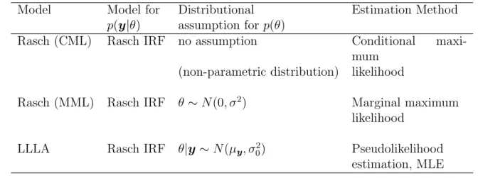
Mixture of conditional normals: demonstrations by simulated data. To demonstrate how the mixture of conditional normal distributions (2.29) in the LLLA model are used to approximate the population latent trait distribution, I use several simulated data from the Rasch model with different specified latent trait distributions.
-4 -2 0 2 4 0.0 0.4 0.8 p(theta|T) p(T) -5 0 5 10 15 0.00 0.10 -4 -2 0 2 4 0.0 0.1 0.2 0.3 0.4 p(theta)
Figure 6. Population latent trait distributions, standard normal, 10 items.
A normal latent trait distribution. In the first simulation, the ability of 1000
model),
θp ∼N(0,1), p= 1, . . . ,1000, (2.35)
and a 10-item test is simulated with difficulty generated from the standard normal distribu-tion, bi ∼N(0,1), i= 1, . . . ,10. The 1000×10 response data matrix is then generated from
the Rasch model.
The persons are grouped according to their total scores into 11 groups, and the histogram of the total scores is shown in the middle panel of Figure 6. The persons in the same total-score group would have the same conditional latent trait distribution p(θ|y) = p(θ|T) =N(σ2
0T, σ02), andσ20 is estimated by fitting the LLLA model to the data. The upper
panel of Figure 6 shows the conditional distributions p(θ|T) of the 11 groups, represented by the 11 normal curves with the same variance ˆσ2
0 and evenly spaced means ˆµT = ˆσ02T. In
the lower panel of Figure 6, the conditional latent distribution for each group of the upper panel is weighted by the corresponding group probability from the middle panel, resulting in p(θ|T)p(T) as shown by the thin solid curves. These weighted conditional distributions are summed up to produce the mixture-of-normal latent trait distribution ˆp(θ) as assumed by the LLLA model, which is shown by the thick solid curve. The true latent trait distribution p(θ) from which the data are simulated is the standard normal distribution, as shown by the thick dashed curve in the lower panel of Figure 6. We can see that the estimated latent trait distribution (the mixture of 11 normals) produced by the LLLA model is very close to the true latent trait distribution, so the mixture-of-normal distribution is a good approximation of the true latent distribution in this data set.
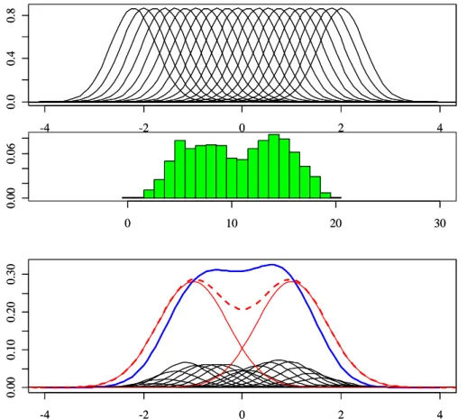
A bi-modal normal mixture latent trait distribution. In the second
simula-tion, we deviate from using a homogeneous latent trait distribution as used in the previous simulation, and generate a heterogeneous population of persons. The ability of 1000 persons
are simulated from a mixture of two normal distributions θp ∼ 1 2N(−1,1) + 1 2N(1,1), p= 1, . . . ,1000. (2.36) The true latent trait distribution p(θ) is shown as the bimodal thick dashed curve in the lower panel of Figure 7, and the two normal components are also shown as the two thin solid curves. -4 -2 0 2 4 0.0 0.4 0.8 0 10 20 30 0.00 0.06 -4 -2 0 2 4 0.00 0.10 0.20 0.30 -4 -2 0 2 4 0.0 0.4 0.8 p(theta|T) p(T) 0 10 20 30 0.00 0.06 -4 -2 0 2 4 0.00 0.10 0.20 0.30 p(theta)
Figure 7. Population latent trait distributions, two-component mixture of normal, 10 items.
The same 10-item test with difficulty generated from the standard normal distribu-tion,bi ∼N(0,1), i= 1, . . . ,10, as in the previous simulation is used, and the response data
matrix is generated from the Rasch model. While the conditional distributions p(θ|T) are similar to those in the previous simulation (compare upper panels of Figure 6 and Figure 7), the distribution of the total scores p(T) now is a different distribution with a bi-modal
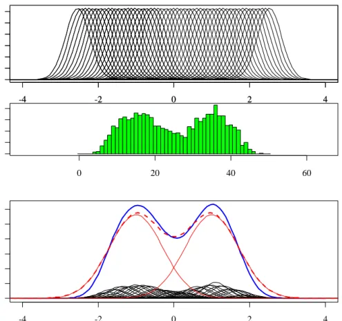
-4 -2 0 2 4 0.0 0.4 0.8 1.2 p(theta|T) -4 -2 0 2 4 0.0 0.4 0.8 1.2 p(T) 0 20 40 60 0.00 0.03 -4 -2 0 2 4 0.00 0.10 0.20 0.30 p(theta)
Figure 8. Population latent trait distributions, two-component mixture of normal, 50 items.
feature (compare middle panels of Figure 6 and Figure 7). The resulting mixture-of-normal latent trait distribution ˆp(θ) produced by fitting the LLLA model (Figure 7, lower panel, thick solid curve) also has a bi-modal feature. Although the approximation of ˆp(θ) to p(θ) in this data set is not as good as shown in the previous simulation, it is better than using a normal distribution, as assumed in the MML Rasch model, to approximate the true latent trait distribution.
If we increase the number of test items to 50, with difficulty generated from the standard normal distribution, the results are shown in Figure 8. The persons are now grouped into 51 groups according to the total scores, and the shape of p(T) has a better resemblance of the latent trait distribution than in the 10-item test. The conditional distribution p(θ|y) has smaller variance σ2
0 than in the 10-item test. The resulting mixture-of-normal latent
solid curve) is now a much better approximation to the true latent trait distribution (Figure 8, lower panel, thick dashed curve).
As demonstrated by the simulation studies, the LLLA model has a greater flexibility in describing the latent trait distribution than the MML Rasch model. When the assump-tions of the MML Rasch model are true (i.e., the latent trait follows a normal distribution), the LLLA model will produce a latent trait distribution very close to the true distribution; in this case we expect the LLLA model will have a performance nearly as good as the MML Rasch model. When the assumption of the MML Rasch model on the latent trait distribu-tion is violated and the latent trait follows a distribudistribu-tion other than a normal distribudistribu-tion, the LLLA model will have a better approximation on the latent trait distribution than the MML Rasch model.
Chapter 3
Pseudolikelihood Estimation
It is known that maximum likelihood estimation can be computationally prohibitive for many models. LLLA models for data sets with large numbers of items fall into this category. Pseudolikelihood estimation (PLE) is a computationally efficient alternative estimation pro-cedure to MLE. The idea of pseudolikelihood estimation was originated by Besag (1975) for spatial data analysis. Arnold and Strauss (1991) proved the consistency and asymp-totic normality of the pseudolikelihood estimator, and it was pointed out that PLE will be less efficient than MLE (see also Geys, Molenberghs, and Ryan (2002a)). Strauss (1992) demonstrated how to use logistic regression procedures to maximize the pseudolikelihood function for different models, and interestingly, the Rasch model was among the examples he discussed. Zwinderman (1995) proposed a pseudolikelihood method for Rasch models based on comparing responses to pairs of items irrespective of other items. Smit and Kel-derman (2000) used pseudolikelihood estimation for the Rasch model for dichotomous items and a single latent trait, and their simulation results show the strong similarity between the pseudolikelihood estimates and those from the conditional maximum likelihood estimation. Most recently, the pseudolikelihood estimation of LLLA model in Anderson, Li, and Vermunt (2007) is directly related to my thesis. In that paper, I implemented in R the pseudolike-lihood estimation procedures for the LLLA model for dichotomous and polytomous items, with single or many latent traits.
In this section, I will first introduce the maximum likelihood estimation procedure for the LLLA model and point out its limitation in terms of computation. Subsequently, I will give the definition of a pseudolikelihood function and derive the pseudolikelihood function used for the LLLA model. I will show how to maximize the pseudolikelihood function by using logistic regression, so that we can conduct the pseudolikelihood estimation (PLE). Finally I will present ways to get correct standard errors for the PLE.