Feature Model Synthesis

by

Steven She

A thesis

presented to the University of Waterloo in fulfillment of the

thesis requirement for the degree of Doctor of Philosophy

in

Electrical and Computer Engineering

Waterloo, Ontario, Canada, 2013

I hereby declare that I am the sole author of this thesis. This is a true copy of the thesis, including any required final revisions, as accepted by my examiners.

Variability provides the ability to adapt and customize a software system’s artifacts for a particular context or circumstance. Variability enables code reuse, but its mechanisms are often tangled within a software artifact or scattered over multiple artifacts. This makes the system harder to maintain for developers, and harder to understand for users that configure the software.

Feature models provide a centralized source for describing the variability in a software system. A feature model consists of a hierarchy of features—the common and variable system characteristics—with constraints between features. Constructing a feature model, however, is a arduous and time-consuming manual process.

We developed two techniques for feature model synthesis. The first, FEATURE-GRAPH -EXTRACTION, is an automated algorithm for extracting a feature graph from a proposi-tional formula in either conjunctive normal form (CNF), or disjunctive normal form (DNF). A feature graph describes all feature diagrams that are complete with respect to the input. We evaluated our algorithms against related synthesis algorithms and found that our CNF variant was significantly faster than the previous comparable technique, and the DNF algorithm performed similarly to a comparable, but newer technique, with the exception of several models where our algorithm was faster.

The second, FEATURE-TREE-SYNTHESIS, is a semi-automated technique for building a feature model given a feature graph. This technique uses both logical constraints and text to address the most challenging part of feature model synthesis—constructing the feature hierarchy—by ranking potential parents of a feature with a textual similarity heuristic. We found that the procedure effectively reduced a modeler’s choices from thousands, to five or less when synthesizing the Linux and eCos variability models. Our third contribution is the analysis of Kconfig—a language similar to feature modeling used to specify the variability model of the Linux kernel. While large feature models are reportedly used in industry, these models have not been available to the research community for benchmarking feature model analysis and synthesis techniques. We compare Kconfig to feature modeling, reverse engineer formal semantics, and translate 12 open-source Kconfig models—including the Linux model with over 6000 features—to

I would like to thank Professors Krzysztof Czarnecki and Andrzej W ˛asowski for providing the guidance and direction that has led to the completion of this dissertation.

Thank you to my colleagues in the Generative Software Development Lab and co-authors: Thorsten Berger, Rafael Lotufo, Yingfei Xiong, and Nele Andersen. A special thanks to Thorsten Berger for the many discussions that have contributed to the work in this thesis.

Finally, thank you to my friends and family—this work would not have been possible without their support.

List of Tables ix

List of Figures xii

1 Introduction 1 1.1 Thesis Statement . . . 9 1.2 Contributions . . . 10 1.3 Publications . . . 11 1.4 Thesis Organization. . . 12 2 Background 13 2.1 Feature Modeling . . . 14 2.1.1 Configuration Semantics . . . 16 2.1.2 Domain Semantics . . . 20 2.1.3 Tool Support . . . 22

2.1.4 Extended Feature Models. . . 23

2.2 Other Variability Modeling Languages . . . 25

2.2.1 Decision Modeling . . . 26

2.2.2 Common Variability Language (CVL) . . . 27

2.2.3 Concept Modeling . . . 27

2.2.4 Component Definition Language (CDL) . . . 28

2.3 Software Product Lines. . . 28

2.4 Feature-Oriented Software Development . . . 29

3 Scenarios and Requirements 31 3.1 Overview of Feature Model Synthesis . . . 31

3.2 Scenario Criteria. . . 36

3.3 Scenarios . . . 38

3.3.1 Scenario 1: Synthesis From a Configurable Platform . . . 38

3.3.2 Scenario 2: Synthesis from Variants . . . 42

3.3.4 Scenario 4: Feature Model Merge Workflows. . . 44

3.4 Discussion and Requirements for Feature Model Synthesis . . . 45

3.5 Scenario Conclusions . . . 48

4 Real World Variability Models 50 4.1 Kconfig Language . . . 51

4.2 Abstract Syntax . . . 56

4.2.1 Configs . . . 56

4.2.2 Choices. . . 58

4.2.3 Identifiers and Expressions . . . 58

4.3 Mapping to Feature Modeling Concepts . . . 58

4.3.1 Hierarchy . . . 60

4.3.2 Feature Groups . . . 60

4.3.3 Feature Constraints . . . 62

4.3.4 Feature Descriptions and Code Mappings . . . 63

4.4 Comparison with Available Feature Models . . . 63

4.4.1 Kconfig Models . . . 64 4.4.2 SPLOT Models . . . 65 4.4.3 Model Structure . . . 65 4.4.4 Feature Groups . . . 70 4.4.5 Cross-Tree Constraints . . . 73 4.4.6 Qualitative Characteristics . . . 74

4.5 Tooling: Linux Variability Analysis Tools . . . 76

4.6 Kconfig Semantics. . . 77

5 Feature Graph Extraction 78 5.1 Motivation and Scenarios . . . 79

5.2 Defining the Feature Model and Feature Graph Synthesis Problem . . . . 81

5.3 Fge: Feature Graph Extraction Algorithm . . . 84

5.4 Fge-CNF: CNF Formula as Input . . . 89

5.5 Fge-DNF: DNF Formula as Input . . . 90

5.6 Fge-BDD: Binary Decision Diagrams as Input . . . 92

5.7 Fge-FCA: Formal Concept Analysis-Based . . . 94

5.8 Selecting a Feature Diagram from a Feature Graph. . . 97

5.9 Experimental Evaluation. . . 97

5.9.1 Goal Definition . . . 98

5.9.2 Hypothesis Formulation. . . 99

5.9.4 Selection of Subjects. . . 100

5.9.5 Experiment Design. . . 102

5.9.6 Operation . . . 103

5.9.7 Results: Fge-CNF Evaluation. . . 105

5.9.8 Results: Fge-DNF Evaluation. . . 112

5.9.9 Hypothesis Testing . . . 116

5.9.10 Threats to Validity . . . 118

5.9.11 Conclusions . . . 118

6 Feature Model Synthesis 120 6.1 Introduction . . . 121

6.2 Overview . . . 124

6.3 Feature Tree Synthesis . . . 127

6.3.1 Building the Feature Hierarchy . . . 127

6.3.2 Feature Groups and Cross-Tree Constraints . . . 130

6.4 Experimental Evaluation. . . 131

6.4.1 Input Data Characteristics . . . 132

6.4.2 Effectiveness of Parent Heuristics . . . 134

6.4.3 Feature Groups . . . 137

6.4.4 Threats to Validity . . . 139

6.5 Conclusions. . . 140

7 Related Synthesis Techniques 141 7.1 DAG Recovery Techniques . . . 144

7.2 Clustering-Based Tree Recovery Techniques . . . 147

7.3 Tree Selection Techniques . . . 149

8 Conclusions 153 8.1 Future Work . . . 154 8.2 Summary . . . 156 Bibliography 158

Appendices

170

A.3 Valuation Functions. . . 172

2.1 Concrete syntax of feature diagrams and the mapping to propositional logic (adapted from[Käs10],[ACSW12],[Ber12]) . . . 17 3.1 Breakdown of artifacts in variability-rich software . . . 33 3.2 Scenario summary . . . 41 4.1 Mapping of concepts between Kconfig and feature modeling (adapted

from[BSL+12]) . . . 59 5.1 Running times (in ms) of the FGE-BDD and FGE-CNF on input derived

from randomly generated models and Linux . . . 107 5.2 Group computation runtimes for SPLOT models that took more than a

second on FGE-BDD . . . 109

5.3 Group computation runtimes for FGE-CNF on SPLOT models that timed

out for FGE-BDD (i.e., took more than 90s) . . . 110

5.4 t-test results for the real world dataset . . . 117 7.1 Summary of related feature model synthesis techniques . . . 142

1.1 Graphical configurators for feature models . . . 2

1.2 Feature model of a model phone product line . . . 3

1.3 Subset of legal configurations of the mobile phone feature model . . . . 3

1.4 Steps for software migration to SPLs (adapted from[Beu06]). . . 4

1.5 Abstract steps in a feature-oriented re-engineering of a software system 5 1.6 Snippets of a FreeBSD variable artifacts . . . 6

1.7 Two feature models with the same set of legal configurations[SLB+11] 7 1.8 Feature models that describe different configurations from Figure 1.7 . . 8

2.1 Power management feature model[SLB+11] . . . 14

2.2 Propositional translation of the feature model in Figure 2.1 . . . 19

2.3 Feature models that describe the same configurations, but have different domain semantics . . . 21

2.4 A feature model of the Journalling Flash File System (JFFS2) with a feature attribute[BSL+10b,BSL+12] . . . 24

2.5 VSpec tree in CVL (adapted from[Obj12]) . . . 26

2.6 Clafer model of the Printer from Figure 2.5 . . . 27

2.7 The problem space, mapping and solution space in SPLs (adapted from [Cza04]) . . . 28

3.1 Variability analysis and feature model synthesis . . . 32

3.2 Different feature diagrams, and a feature graph, with the same configu-ration semantics describing the same set of configuconfigu-rations . . . 34

3.3 Abstract workflows for feature model synthesis. . . 35

3.4 Property of a transformation step . . . 37

3.5 Scenario workflows . . . 39

3.5 Scenario workflows (cont.) . . . 40

3.6 Another example of two feature models with the same configurations. . 47

4.1 Kconfig excerpt adapted from[BSL+10b] . . . 52

4.3 Evaluating operators and literals in the three-valued logic of Kconfig . . 55

4.4 Specifying Hierarchy in Kconfig . . . 60

4.5 Feature group representation in Kconfig . . . 60

4.6 Feature group rendering in xconfig configurator . . . 61

4.7 A conditionally derived config in the Linux kernel . . . 62

4.8 Proportion of configs that violate hierarchy rules in the Kconfig models . 66 4.9 Size of Kconfig and SPLOT models . . . 67

4.10 Feature types in the Kconfig models . . . 68

4.11 Leaf depths for the Kconfig models ordered by model size . . . 69

4.12 Structure of the Kconfig and SPLOT models across all features in the dataset. . . 70

4.13 Feature groups in Kconfig models . . . 71

4.14 Feature groups and CTCR across all features in SPLOT and Kconfig models 72 4.15 Proportion of derived and conditionally derived configs in the Kconfig models. . . 73

4.16 Characterization of a small sample of features in the Linux v2.6.28.6 kernel . . . 74

4.17 Representation of Kconfig’s three values using two Boolean variables . . 76

5.1 Maximal feature diagrams and a feature graph . . . 82

5.2 Generic feature graph extraction algorithm, adapted from [ACSW12, CW07]. . . 85

5.3 Translation of a DNF formula to a BIP problem for identifyingOR-groups 93 5.4 Formal context and its attribute concepts . . . 95

5.5 SPLOT model dataset properties . . . 101

5.6 Running times for FGE-BDD and FGE-CNF on the input derived from randomly generated models. . . 106

5.7 Running times for group computation in FGE-BDD and FGE-CNF on input derived from SPLOT models . . . 108

5.8 Detected feature groups . . . 111

5.9 Distribution ofOR-group computation times for FGE-DNF and FGE-FCA . 112 5.10 Group computation times for FGE-DNF and FGE-FCA . . . 113

5.11 The effect of the number of configurations forOR-group computation on FGE-DNF. . . 114

5.12 A snippet of the original Smart Phone SPL. . . 115

6.1 Example input for feature model synthesis. . . 123

6.2 Mockup of the two parent candidate lists . . . 125

6.4 Implication graph of the dependencies in Figure 6.1. . . 128 6.5 Characterization of descriptions, transitive implications (dark grey) and

direct implications (white) for eCos, FreeBSD, the FreeBSD reference model, and Linux . . . 132 6.6 Robustness of RIFs for theprioritizing(black) andnon-prioritizing(gray)

orders under complete and incomplete data. . . 135 6.7 The top RAFs needed for a user to have a 75% chance of finding the

reference parent under complete and incomplete descriptions. . . 136 6.8 Reference groups detected asxor- (black) ormutex-groups (grey) under

complete and incomplete exclusions . . . 137 7.1 Workflows for DAG and Tree Recovery Techniques . . . 143

Introduction

Variability provides the ability to adapt and customize a software system’s artifacts for a particular context or circumstance [vGBS01]. Variability enables code reuse, but its mechanisms are often tangled within an artifact or scattered over multiple artifacts that span the problem space, solution space, or the mapping connecting the two spaces.Variability-rich software, in particular, pose a challenge for developers and users. Developers need to understand the impact of a change in order to add new features or dependencies to existing features. For users that configure the software system, complex feature interactions can lead to unsatisfied dependencies.

Feature models(FMs), first introduced by Kang et al.[KCH+90], describesfeatures—the common or variable characteristics of the products in a SPL—as a visual hierarchy with additional constraints between features. Since feature models were first introduced, they have been used in a wide variety of tasks such as domain analysis[KCH+90], model management[Ach11], describing design or implementation constraints in variability-rich software[CE00], and product configuration. Feature model configurators provides intuitive graphical interfaces for configuring features and understanding their depen-dencies (Figure1.1).

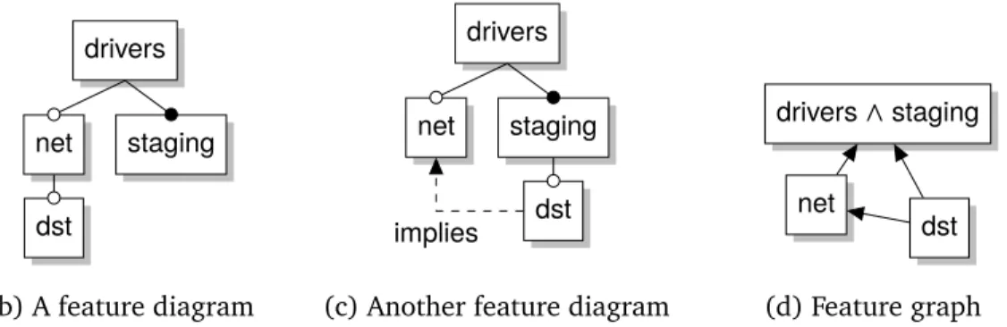
Figure 1.2 shows a feature model of a mobile phone product line. Features are represented as rectangles and may beoptional—denoted by an empty circle at the top— ormandatory—denoted by a filled circle. An edge from one feature to another denotes a dependency, where a solid line denotes the feature hierarchy, and a dashed line with an arrow is across-tree implies edge. Cross-tree excludes edgescan also exist in the diagram, but are not shown in this particular example. Constraints between sibling features can also be specified as part of afeature group. AnXOR-group, shown with a clear arc, denotes that exactly one member of the group must be selected if its parent is selected. OR-groups, shown with a filled arc, where one or more members must be selected, and

(a) A graphical configurator for the Linux kernel

(b) Variant matrix editor from pure::variants[pur12] Figure 1.1: Graphical configurators for feature models

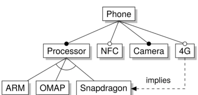
Phone

Processor NFC Camera 4G

ARM OMAP Snapdragon

implies

Figure 1.2: Feature model of a model phone product line { Phone, Processor, ARM, Camera },

{ Phone, Processor, ARM, Camera, NFC }, { Phone, Processor, OMAP, Camera },

{ Phone, Processor, Snapdragon, Camera, 4G }, . . .

Figure 1.3: Subset of legal configurations of the mobile phone feature model

MUTEX-groups, where zero or one members must be selected, also exist, but are not shown in the figure. The graphical components—i.e., the feature hierarchy, feature groups, and cross-tree edges—form thefeature diagram. A feature model consists of the feature diagram and an additionalcross-tree formula to describe constraints that could not be represented in the diagram. The configuration semantics of a feature model is a set oflegal configurationsdefined by the satisfying assignments for its translation to propositional logic[Bat05]. For example, a subset of the legal configurations for the feature model in Figure1.2is the set of configurations in Figure1.3.

Since their introduction, feature models have become widely used in literature and in industry. At the time of writing, the SPLOT model repository contained over 250 feature models gathered from academia, or contributed by industry1 _{[MBC09]. While}

these models originate from different sources, the models are all small in size, with the largest model having 280 features2. Large feature models with hundreds, and even thousands of features exist in industry. However, these model are not available to the research community[MBC09,BSRC10]. Open source, variability rich projects, such as the Linux or eCos kernels have large, explicitly defined variability models. Linux uses the Kconfig language to specify its variability model and eCos has the Component Definition Language (CDL). These language are quite similar to feature modeling and

1_{http://splot-research.org} 2_{As of December 9, 2012}

Existing System (Pre-SPL)

Product Relation Pattern Matching

Transition Scenario Identified

Variability Analysis

Feature Model Synthesis

(Model Building)

Feature-Oriented System (SPL)

Figure 1.4: Steps for software migration to SPLs (adapted from[Beu06]) their models can be interpreted as feature models[SSSPS07,SLB+10,BSL+10b]. We derived a mapping from Kconfig concepts to feature modeling and identified unique concepts of Kconfig[SLB+10,BSL+10b]. We reverse engineered formal semantics for the Kconfig language[SB10]and used the semantics to translate a Kconfig model to propositional logic. We describe our research on the Kconfig language in Chapter4. Figure1.4 is a workflow by Beuche for migrating a software system to a SPL archi-tecture [Beu06]. In the figure, product relation pattern matching is the process of identifying the relation between the products in the envisioned product line. This process involves identifying shared software assets, similarities between user-facing features, and whether the existing system used any form of systematic variability man-agement between products. Next, atransition scenario that describes the goal of the migration process is identified. For example, one scenario involves merging separate products into a product line. Another scenario involves improving reuse between software assets in an existing product line. Chapter3describes several feature model synthesis scenarios that we gathered from literature and from industry experience reports[SCW12]. Variability analysisidentifies features and variability in the project

Existing System Features, Valid Configurations,

andStructural Information1

Feature Model

Feature-Oriented System

Variability Analysis

e.g., feature location, dependency mining

Feature Model Synthesis

Re-Engineering Software Artifacts

1

optional information used to guide feature hierarchy construction.

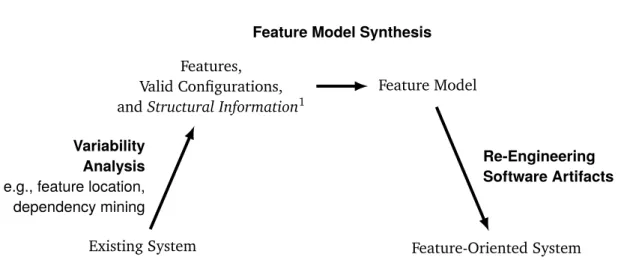
Figure 1.5: Abstract steps in a feature-oriented re-engineering of a software system artifacts. The last step of the process isfeature model synthesis, the focus of this thesis. Feature model synthesis involves the construction and design of a feature model using the features and variability data identified in the previous steps of the workflow. In Beuche’s original slides[Beu06], he describe the variability analysis and model building stages as iterative and incremental. In this dissertation, we address a one-way, batch process for feature model synthesis. We leave the incremental synthesis process as future work.

We elaborate on the variability analysis and feature model synthesis stages in Figure1.5. Variability analysis is performed by a domain export to identify features and variability in a system with automated tooling such as feature identification and location[DRGP11]. Valid configurations can be identified with either dependency mining[BSL+10a,Käs10], or extracting configurations from variants[RPK11]. The analysis stage also involves identifying structural information for the synthesis technique if needed. In our synthesis technique, we use supplemental feature descriptions to rank potential parents of a features (Chapter6). We give other examples of analysis techniques for extracting the needed synthesis input in Chapter 3. In the feature model synthesis step, a domain expert constructs and designs a feature model given the identified features, valid configurations, and any supplemental information. This step is tool-assisted, since it requires user input to build and design a model. After a feature model is constructed, the remaining software artifacts in the project, such as the build system or source code, is adapted to use the synthesized feature model as its source for variability. In this thesis, we address the middle step in this process: feature model synthesis.

STACK enables the stack(9) facility. . . stack(9) will also be compiled in automatically if DDB(4) is compiled into the kernel.

(a) Documentation with a dependency betweenSTACKandDDB

#ifdef DDB #ifndef KDB

#error KDB must be enabled for DDB to work! #endif

#endif

(b) Code snippet with a dependency betweenDDBandKDB

# Debugging for use in -current

options KDB # Enable kernel debugger support. options DDB # Support DDB.

options GDB # Support remote GDB. ...

nooption NATIVE options MCLSHIFT=12

(c) Snippet of a hardware configuration for i386 XEN support

{OS,staging} {OS,staging,net} {OS,staging,net,dst}

(a) A set of configurations

OS net staging dst (b) A FM OS net staging dst implies (c) Another FM

Figure 1.7: Two feature models with the same set of legal configurations[SLB+11]

Next, we will describe a concrete scenario involving feature model synthesis. The FreeBSD kernel is a system without a feature model and could benefit from a feature-oriented re-engineering. Variability is scattered over a mixture of variable artifacts and instances. Features and dependencies are described in an ad-hoc manner—features are scattered in documentation and dependencies are hidden in code and feature configurations for different hardware architectures and devices. Figure 1.6a is a snippet from documentation in FreeBSD describing a dependency between two features:

STACK and DDB. Dependencies involving the DDB feature is not localized to just

documentation; a dependency betweenDDBandKDBalso exists in the FreeBSD source code (Figure1.6b). A configuration in FreeBSD is simply a list of features and their values (Figure1.6c). A user looking to understand the dependencies of theDDBfeature would have to examine configuration templates, feature documentation, and source code. FreeBSD is a system that would benefit from an explicit representation of features and their dependencies.

Re-engineering the variability of a software system is just one scenario involving feature model synthesis. Feature models can also be synthesized for domain analysis from requirements, drive configuration of existing and future products from code variants, or as part of a model management operation such as a model merge from a set of other feature models[SCW12]. We elaborate on these scenarios in Chapter3.

Feature models provide an intuitive graphical notation for describing a set of legal configurations. However, given a set of configurations, there could be many different feature models that describe these configurations. For example, Figures 1.7b and 1.7cboth describe the same set of configurations in Figure1.7a. Other models could describe more configurations (Figure1.8a), or less configurations (Figure1.8b). Even though the feature model in Figure1.8adescribes more configurations than the input,

OS

net dst staging (a) More configurations

OS net staging dst (b) Less configurations OS net staging dst (c) Arbitrary configurations

Figure 1.8: Feature models that describe different configurations from Figure1.7 this model could very well describe best what the modeler intended. For example, synthesis scenarios involving domain analysis from requirements, or synthesizing a feature model from individual variants to describe a product line require a feature model that is more general than the input configurations. Our feature model synthesis algorithms ensure that the synthesized feature model that is weaker than the input configurations. In other words, the configurations in the synthesized feature model are a superset of the configurations in the input, making the model complete with respect to the input configurations. Additional constraints can be added in the stage following feature model synthesis.

We developed an efficient, automated algorithm calledFeature Graph Extraction(FGE) that recovers a feature model that is complete with respect to the input configurations. FGE takes an input propositional formula, and extracts a specialfeature graph that describes all possible feature diagrams that are complete with respect to the input configurations, orsound with respect to the input dependencies [ACSW12, CW07]. Our algorithm is capable of synthesizing a feature graph from a set of features, a set of dependencies expressed as a formula in conjunctive normal form (CNF), or as a set of configurations expressed as a formula in disjunctive normal form (DNF). FGE acts as an intermediate step in a larger feature model synthesis scenario. For example, the resulting feature graph can be used as input to an interactive feature model building tool [JKW08] or as part of a feature model merge or projection op-eration[Ach11]. We use FGE as the basis of our own semi-automated feature model synthesis technique[SLB+11]. We describe FGEin Chapter5.

The feature graph recovered by FGE representsa setof feature diagrams and is not a valid feature diagram on its own. A distinct feature tree and a set of feature groups have to be selected from the feature graph for it be a valid feature model. If we look at

the two feature models in Figures1.7band1.7cagain, both feature models describe the same set of input configurations. However, the two feature models differ in their feature hierarchies. The feature hierarchy and arrangement of feature groups reflect the domain semantics of the feature model[SLB+11]. As an example, let’s assume that selecting thenetfeature enables networking support,dstenables distributed storage support, and that subfeatures ofstagingdescribes experimental features. Ifdstis an experimental feature, placing the feature understaging is more appropriate (Figure1.7c). However, ifdstis a stable feature, then placing it undernetis more appropriate (Figure1.7b). In this example, the appropriate feature hierarchy is determined by the meaning, or domain semantics of its features.

Determining the location of a feature in the feature hierarchy becomes a significant challenge when synthesizing a feature model with thousands of features. We developed a semi-automated technique to identify relevant parents for a feature by using logical dependencies and a textual similarity heuristic [SLB+11]. We use this technique to reverse engineer a feature model for a portion of the FreeBSD kernel and evaluated the effectiveness of our technique by comparing the results of our heuristic with reference feature models extracted from the Linux, eCos, and a portion of the FreeBSD kernel. We discuss this technique in Chapter6.

Our FM synthesis techniques assumes features, and valid feature combinations ex-pressed as a set of dependencies or configurations as input. Other FM synthesis tech-niques exist that use different inputs, from requirements documents[ASB+08,NE08b]

to semi-structured product descriptions [ACP+12]. We discuss related FM synthesis techniques in Chapter7.

1.1 Thesis Statement

We synthesize large-scale feature models with thousands of features by using SAT-based reasoning on propositional formulas and suggest a feature hierarchy by combining logical reasoning with textual similarity heuristics.

We establish this thesis by evaluating our synthesis algorithms against comparable algorithms on input derived from generated and real-world feature models. We evaluate our textual similarity heuristic on input derived from the Linux, eCos, and FreeBSD kernels.

1.2 Contributions

This thesis claims the following contributions:

• We collected feature model synthesis scenarios from literature and industry experience reports. We classify and show the workflows of the individual scenarios and derive an abstract workflow and requirements for feature model synthesis algorithms [SCW12]. Chapter 3 presents the scenarios and requirements for feature model synthesis algorithms.

• We analyzed the Kconfig variability modeling language and derived formal seman-tics[SB10], and a mapping from Kconfig to feature modeling[SLB+10,BSL+10b]. The Kconfig language developed specifically for Linux to specify its variability model. This model has over 6000 features and provides the largest benchmark for feature model analysis and synthesis tools. The Kconfig analysis tools con-tributed to the analysis of the evolution of Linux over 21 releases from v2.6.12 to v2.6.32[LSB+10], and extracted models from 11 open-source projects that use Kconfig[BSL+12]. We discuss the Kconfig language in Chapter4.

• We introduce the automated FEATURE-GRAPH-EXTRACTION algorithm [SRA+13,

ACSW12] in Chapter 5. Given input as a set of features, and a propositional

formula in either conjunctive normal form (CNF) or disjunctive normal form (DNF), this algorithm recovers a graph that describes all feature diagrams that entails the input. Our evaluation found that the CNF variant perform 10 to 1000 faster than a previous BDD-based algorithm [CW07] and could handle much larger input, including input derived from the Linux kernel. The DNF variant was comparable to a formal concept analysis-based algorithm by Ryssel et

al.[RPK11].

• In Chapter 6, we describe our semi-automated FEATURE-TREE-SYNTHESIS algo-rithm[SLB+11]. This algorithm takes a set of features, dependencies, and feature descriptions to present potential parents for feature to help a modeler build the feature hierarchy. Given a feature, FEATURE-TREE-SYNTHESIS creates a list containing the implied features ranked by their textual similarity, and a second list containing all features ranked by their textual similarity for situations where input dependencies may be missing. This algorithm was the first to use both logical dependencies and textual similarity heuristics for feature model synthesis. Our evaluation found that given a feature, the algorithm identified the correct parent for 76% of features in the Linux variability model and 79% of features

from the eCos variability models, and the correct parent appeared in the top 3% to 6% of all features.

1.3 Publications

[SLB+10] S. She, R. Lotufo, T. Berger, A. W ˛asowski, and K. Czarnecki, “The variability model of the linux kernel,” in VaMoS, 2010.

[SB10] S. She and T. Berger, “Formal semantics of the Kconfig language,” Genera-tive Software Development Lab, University of Waterloo, Technical Note, 2010. [Online]. Available: http://gsd.uwaterloo.ca/sites/default/files/ kconfig_semantics.pdf.

[BSL+10a] T. Berger, S. She, R. Lotufo, K. Czarnecki, and A. W ˛asowski, “Feature-to-code mapping in two large product lines,” in Software Product Lines: Going Beyond, SPLC, 2010.

[BSL+10b] T. Berger, S. She, R. Lotufo, A. W ˛asowski, and K. Czarnecki, “Variability modeling in the real: a perspective from the operating systems domain,” in ASE, 2010.

[SLB+11] S. She, R. Lotufo, T. Berger, A. W ˛asowski, and K. Czarnecki, “Reverse engineering feature models,” in ICSE, 2011.

[BSL+12] T. Berger, S. She, R. Lotufo, A. W ˛asowski, and K. Czarnecki, “Variability modeling in the systems software domain,” Generative Software Devel-opment Lab, University of Waterloo, Tech. Rep. GSDLAB-TR 2012-07-06, 2012. [Online]. Available: http://gsd.uwaterloo.ca/sites/default/files/ vm-2012-berger.pdf.

[ACSW12] N. Andersen, K. Czarnecki, S. She, and A. W ˛asowski, “Efficient synthesis of

feature models,” in SPLC, 2012.

[XHSC12] Y. Xiong, A. Hubaux, S. She, and K. Czarnecki, “Generating range fixes for

software configuration,” in ICSE 2012.

[SCW12] S. She, K. Czarnecki, and A. W ˛asowski, “Usage scenarios for feature model

[SRA+13] S. She, U. Ryssel, N. Andersen, A. W ˛asowski, and K. Czarnecki, “Efficient synthesis of feature models,” submitted for review in Information and Software Technology, 2013.

1.4 Thesis Organization

In this chapter, we described the motivation behind feature model synthesis and pre-sented an overview of our work. Chapter 2describes feature models in detail, and provides background on variability modeling and software product lines. Chapter3 discusses feature model synthesis scenarios and derives requirements for synthesis tech-niques from the scenarios. Chapter4discusses the Kconfig language—the variability modeling language developed and used by the Linux kernel—and compares the prop-erties of 12 Kconfig models against a set of 267 published feature models. Chapter5 describes the first synthesis algorithm, FEATURE-GRAPH-EXTRACTION, that given a set of features and dependencies, extracts a special feature graph describing all feature diagrams that are sound with respect to the input dependencies. Chapter6describes a semi-automated algorithm that takes a feature graph and recovers a distinct feature model. Chapter7discusses related synthesis techniques, and Chapter8concludes with ideas for future work.

Background

Large software systems such as operating systems, automotive software, or embedded systems, contain significant variability. This variability is often scattered over multiple artifacts such as optional requirements, high level features, or low level run-time options. Variability in code often takes the form of code fragments annotated with a condition. A variability model makes the variability in a software system explicit. Feature modeling is one form of variability modeling. Feature modeling was first introduced in 1990 as part of the feature-oriented domain analysis (FODA)[KCH+90]. Since then, feature modeling has become popular due to its ability to codify the critical information for reuse (e.g., variation points and variants), simplicity, understandability, and practicality[Kan10]. We discuss feature models in depth in Section2.1.

Feature models are not the only form of variability modeling. For example, the popu-larity of variability modeling has led the Object Management Group (OMG) to work towards a standard called the Common Variability Language (CVL)[Obj12]. Other vari-ability modeling languages include decision modeling[DGR11]and Clafer[BCW10]. The open-source community has developed the Kconfig[Zc]and Component Definition Languages (CDL)[BV00]. We discuss CVL, decision modeling and other variability modeling languages in the following section. We defer the discussion of the Kconfig language to Chapter4.

Chapter Organization Section 2.1 introduces feature models and discusses their configuration semantics, domain semantics, and tool support. We briefly discuss ex-tended feature models, e.g., feature attributes, and non-propositional feature models. In Section2.2, we discuss variability modeling languages other than feature modeling. These include decision models, the Common Variability Language (CVL), Clafer, and

pm

acpi cpu_freq

acpi_system cpu_hotplug performance powersave

x x

excludes

implies implies

powersave∧acpi→cpu_hotplug

Figure 2.1: Power management feature model [SLB+11]

the Component Definition Language (CDL). Sections2.3 and2.4 describe how fea-ture modeling fits into Software Product Lines (SPLs) and Feafea-ture-Oriented Software Development (FOSD).

2.1 Feature Modeling

Feature modeling was introduced by Kang et al. as part of feature-oriented domain analysis (FODA)[KCH+90]. A feature model (FM) consists of features arranged in (i) a feature diagram, and (ii) additional constraints between features. Afeatureis some property that is relevant to some stakeholder[CE00].

Thefeature diagramis a visual hierarchy of features. A feature may have subfeatures, i.e., a parent feature may have one or more children features. The topmost feature is called theroot feature and represents the concept described in the feature model. All other features are either solitary or grouped. Solitary features can beoptional—where the feature may or may not be selected if its parent is selected, ormandatory—where the feature must be selected if its parent is selected. Grouped features belong to feature groups that is either aMUTEX-, OR-, or XOR-group. A MUTEX-group requires that either one or none of the grouped features are selected. A OR-group requires that at least one of the grouped features are selected. AnXOR-group requires exactly one grouped

feature be selected. Additional cross-tree constraints in the form ofimpliesandexcludes

edges can shown in the feature diagram. Arbitrary constraints can be added in a cross-tree formula shown below the feature diagram. The feature diagram along with the cross-tree formula form a feature model.

Figure2.1is a feature model of a power management subsystem. In this model,pmis the root feature. Featuresacpiandcpu_freqare optional features ofpm. acpi_system

is a mandatory feature. Featuresperformanceandpowersavebelong in anXOR-group. MUTEX- andOR-groups are not shown in this feature diagram. There are implies edges fromcpu_hotplugtoacpi, andcpu_hotplugtopowersave, and anexcludesedge between

cpu_hotplugandperformance. An additional cross-tree formula is shown below the

diagram.

Definition 2.1. Afeature diagramis a tupleFD= (F,E,(E_m,E_i,E_x),(G_o,G_x,G_m))

where:

• F is a finite set of features,

• E⊆F×F is a set of directed child-parent edges; • E_m⊆E is a set of mandatory edges,

• E_i⊆((F _×F)₋E)is a set ofimpliesedges,

• E_x ⊆2F _{is a set of undirectedexcludesedges where|e|=2 for alle∈E} x;

• G_o,G_x,G_m are sets that contain non-overlapping subsets of E that partici-pate inOR-,XOR-, orMUTEX-groups respectively—each set in any ofG_o,G_x, andG_m is disjoint from any other set inG_o,G_x, andG_m.

The following well-formedness constraints must hold inFD: 1. (F,E)is a rooted tree connecting all features inF.

2. All edges in a group share the same parent, so if g∈G_i fori∈ {o,x,m} and if(f₁,f₂),(f₃,f₄)_∈g, then f₂= f₄.

3. SetsE,E_i,E_x are pairwise disjoint.

Based on the definition above, features not having a mandatory edge are considered

optional features. Feature groups in the diagram are also restricted to onlyOR-, XOR-, andMUTEX-groups. The original feature diagram notation introduced in FODA included onlyXOR-groups with〈1..1〉cardinality[KCH+90]. Czarnecki and Eisenecker extended the feature diagram to includeOR-groups with〈1..n〉cardinality[CE00]. While there are feature diagram notations that allow arbitrary〈m..n〉group cardinalities[SHTB07],

we found that these group cardinalities were very uncommon in practice—in a dataset of 267 feature models contained in a feature model repository[MBC09], none of the models had feature groups with〈m..n_〉cardinalities.

Definition 2.2. Afeature model,FM= (FD,φ), whereFDis the feature diagram andφ is a propositional formula overF.

Feature models have been used to drive product derivation [AC04], domain analy-sis[KCH+90,ASB+08], model management, and describe design and implementation constraints in a software system. At its core, feature models describe variability as a set of legal configurations. In the following section, we define the configuration and domain semantics of a feature model.

2.1.1 Configuration Semantics

The configuration semantics of a feature model is a set of legal configurations—sets of selected features that respect the dependencies entailed by the diagram and the cross-tree constraints. The configuration semantics can be specified via translation to logic[Bat05]. We decompose the configuration semantics of a feature diagram by their graphical components in Table2.1and by using the formal definition in Definition2.1 as follows:

Root Feature The root feature must be present in all configurations forming the following propositional constraint:

r where r is the root of the tree(F,E) (2.1) Child-Parent Implications The feature hierarchy is represented as implications from a child feature to a parent feature. Given a child feature f_c(e.g.,powersave) and a parent feature f_p(e.g.,cpu_freq), the following constraints are added:

^

(c,p)∈E

(c_→p) (2.2)

Mandatory Features The set of edges inE_mrepresent mandatory features—features that must be selected if its parent is selected. Mandatory features add the following

Feature diagram syntax Propositional translation cis an optional subfeature ofp p c (c→p) cis a mandatory subfeature ofp p c (c_→p)_∧(p_→c)

{c1,c2, . . . ,ck}are anXOR-group ofp

p c1 c2 · · · ck 〈1..1_〉 (c1∨. . .∨ck→p)∧ (p→c1∨. . .∨ck)∧ ^ i,j=1..k i6=j (ci → ¬cj) {c₁,c₂, . . . ,c_k}are anOR-group ofp p c₁ c₂ · · · c_k 〈1..k_〉 (c1∨. . .∨ck→p)∧ (p→c1∨. . .∨ck)

{c1,c2, . . . ,ck}are aMUTEX-group ofp

p c1 c2 · · · ck 〈0..1_〉 (c1∨. . .∨ck→p)∧ ^ i,j=1..k i6=j (c_{i → ¬}c_j)

fhas an implies edge tok fandkshare an excludes edge

k f implies (f _→k) f kx x excludes (f _{→ ¬}k)

Table 2.1: Concrete syntax of feature diagrams and the mapping to propositional logic (adapted from [Käs10],[ACSW12],[Ber12])

constraint, in addition to the child-parent implications above:

^

(c,p)∈Em

(p→c) (2.3)

Implies Edges An implies edge in E_i naturally adds an implication to the set of constraints:

^

(f,k)∈Ei

(f →k) (2.4)

Excludes Edges An excludes edge describe a mutual exclusion between two fea-tures. Excludes edges contribute the following constraints:

^

(f,k)∈Ex

(f → ¬k) (2.5)

Feature Groups G_o,G_x,G_msets contains sets of non-overlapping edges that define the OR-, XOR-, MUTEX-groups respectively. Feature groups contribute two kinds of constraints: a requirement that at least one of the group members must be present, and mutual exclusions between group members. OR-groups have the former constraint, MUTEX-groups have the latter constraint, andXOR-groups have both. Feature groups contribute the following constraints:

^ {(c1,p),...,(ck,p)}∈Go∪Gx p→c1∨ · · · ∨ck (2.6) ^ {(c1,p),...,(ck,p)}∈Gm∪Gx    ^ i,j∈{1,...,k}wherei6=j c_{i→ ¬}c_j    (2.7)

Definition 2.3. The functionp(·)translates a feature diagram or a feature model to propositional logic, interpreting features as variable names. For a feature dia-gramFD= (F,E,(E_m,E_i,E_x),(G_o,G_x,G_m)), we define the configuration semantics as:

(acpi → acpi_system∧pm)

∧ (acpi_system → acpi)

∧ (cpu_freq → pm)

∧ (cpu_freq → powersave∨performance)

∧ (cpu_hotplug _→ powersave)

∧ (cpu_hotplug → ¬performance)

∧ (cpu_hotplug → acpi∧cpu_freq)

∧ (powersave → ¬performance)

∧ (powersave → cpu_freq)

∧ (performance → cpu_freq)

∧ (powersave∧acpi → cpu_hotplug)

Figure 2.2: Propositional translation of the feature model in Figure2.1

p(FD) = r _∧ root feature ^ (c,p)∈E (c→p)∧ child-parent implications ^ (f,k)∈I

(f →k)∧ mandatory and implies edges

^ (f,k)∈X (f →¬k)∧ excludes edges ^ {(c1,p),...,(ck,p)} ∈Go∪Gx p→(c₁∨ · · · ∨c_k) ∧ feature groups ^ {(c1,p),..,(ck,p)} ∈Gm∪Gx ^ i,j∈{1,...,k} i6=j (c_i → ¬c_j) (2.8)

where ris the root feature of the tree formed by the features and edges of(F,E). Definition 2.4. Given FM = (FD,φ), the configuration semantics of a feature model,FM, is defined asp(FM) =p(FD)∧φ.

Applying the propositional translation,p(·), to the feature model in Figure2.1results in the formula in Figure2.2. Any satisfying variable assignment to this formula is a legal configuration.

2.1.2 Domain Semantics

Feature models describe a set of legal configurations with its configuration semantics. A second semantics, thedomain semantics(called ontological semantics in[SLB+11]), describe the domain in the structure of the model. The domain semantics describes the meaning of the features and is reflected in a model’s hierarchy and feature group arrangement.

As we saw earlier in Figure1.7, two feature models can describe the same configurations, but have different hierarchies. The different hierarchies convey a different domain semantics. The feature hierarchy is not the only part of a feature model that affects its domain semantics—the feature groups and cross-tree constraints also have an effect. For example, the feature models in Figure2.3all describe the same three configurations:

{cpu_governor,powersave_},

{cpu_governor,powersave,cpu_hotplug}, {cpu_governor,performance}.

The featurespowersave andperformanceare both CPU governors, andcpu_hotplug

controls whether the CPU can be enabled or disabled dynamically. If we examine the feature models in Figure2.3, the models all have the same configuration semantics, but different domain semantics. In Figure2.3a,powersaveandperformanceare grouped together and an excludes edge exists between performance and cpu_hotplug. The features are grouped differently in the feature model in Figure 2.3b. Between the feature diagrams in Figures2.3aand2.3b, the arrangement of features in Figure2.3b matches the domain relations of the features better.

Between Figures 2.3b and 2.3c, the feature grouping and hierarchy are the same, however, the cross-tree constraints are different. How cross-tree constraints are repre-sented in the feature model also impact the domain semantics of the model. Finally, in Figure2.3d, the bi-implies edge (i.e., a shorthand for two implies edges) is redundant in terms of the configuration semantics—the edge may be removed without affecting the modeled set of configurations. However, the model builder may want to include this bi-implies edge to make the relation betweenpowersave andcpu_hotplugexist.

cpu_governor

powersave performance cpu_hotplug

x x

excludes

(a)powersaveandperformanceare in a feature group

cpu_governor

powersave performance cpu_hotplug

bi-implies

(b)performanceandcpu_hotplugare in a feature group

cpu_governor

powersave performance cpu_hotplug

x x

excludes implies

(c) Same hierarchy and feature groups asb, but with different cross-tree constraints

cpu_governor

powersave performance cpu_hotplug

bi-implies

(d) Redundant cross-tree constraint

Figure 2.3: Feature models that describe the same configurations, but have different domain semantics

The domain semantics are reflected in the hierarchy, feature groupings, and cross-tree constraints.

2.1.3 Tool Support

As feature models grow in size and complexity, tool support and automated analysis become a necessity [BPSP04]. Feature modeling tools include graphical configu-rators and automated analysis such as dead feature detection, valid configuration enumeration[BSRC10], fix generation[XHSC12], choice propagation and model com-pletion[WSB+08]. Feature models have support for staged configuration[CHE05b], conflict resolution strategies[NE10], and support for different perspectives and collab-oration for configuration[Hub12].

Examples of feature modeling tools are the FaMa-FW framework and the FAMILIAR domain-specific language. FaMa-FW is a framework for the automated analysis of feature models[TBRC+08]. It supports multiple reasoners, such as BDDs, SAT solvers, or constraint satisfaction problem solvers. FaMa-FW supports operations such as calcu-lating the legal configurations, error detection and explanation. Acher et al. developed FAMILIAR—a domain specific language for reasoning on feature models[Ach11]. FA-MILIAR supports operations such as feature configuration, detecting dead features, and counting or enumerating legal configurations. The key feature of FAMILIAR is its support for composing feature models. It integrates our feature model synthesis algorithm (Chapter5) to perform operations between propositional logic and feature models. We discuss how our synthesis algorithm is used for feature model composition as one of the scenarios in Chapter3.

TVL (Text-based Variability Language) is a language for specifying feature models with a C-like syntax[BCFH10]. TVL offers modularity mechanisms and goes beyond propositional feature models to supports feature cardinalities and attributes. Reasoning on feature models with feature cardinalities and attributes is beyond propositional logic and requires a reasoner such as a constraint satisfaction problem (CSP) solver, model checker, or a satisfiability modulo theories (SMT) solver. We discuss feature cardinalities and attributes in the following section. GUIDSL is another textual feature modeling language that is part of the AHEAD tool suite[Bat05,Bat04].

Pure-systems’ pure::variants1 _{and BigLever Software’s Gears}2 _{are two commercial}

1_{http://www.pure-systems.com/}

feature modeling tools. Both pure::variants and Gears go beyond feature modeling and support other aspects of a software product line workflow. For example, these tools are capable of managing configurations (i.e., variants) and support integration with other software artifacts such as requirements and build systems. We give an introduction to software product lines in Section2.3.

In the open-source community, the Kconfig and Component Definition Languages (CDL) share many similar concepts with feature modeling, such as a feature hierarchy and feature groups[SSSPS07,SLB+10]. Both tools have a graphical configurator. However, unlike feature modeling tools that use reasoners (e.g., BDDs or SAT solvers), Kconfig and CDL tools rely on an imperative implementation for performing configuration validation and conflict resolution. We describe our study on the Kconfig language in Chapter4. For details on the CDL language, refer to Berger’s dissertation[Ber12]and related work[BSL+10b,BSL+12].

2.1.4 Extended Feature Models

Since feature models were first introduced by Kang et al. [KCH+90], feature mod-els have been extended with feature attributes [KCH+90, BSRC10], group cardinal-ities [RBSP02], feature cardinalities [CHE05a], or probabilities [CSW08, She08]. Schobbens et al. derive a new feature diagram notation—varied feature diagram (VFD)—that integrate various feature model extensions into a single feature diagram structure and providing a formal semantics [SHTB07]. We discuss several of these feature modeling extensions in this section.

Feature Attributes Figure2.4 shows a feature model of the Journaling Flash File System, inspired by the Linux variability model. In this model, Debug Level is a mandatory feature with an integer attribute. A cross-tree constraint restricts this attribute to the values: 0, 1 or 2. While a standardized notation for feature attributes in feature models does not exist, an attribute consists of at least a name, a domain (e.g., integer, real, string), and a value[BSRC10]. The notation in Figure2.4is derived from the original feature model notation from FODA[KCH+90]. Benavides et al. propose an alternative notation where attributes are attached to features with a separate box and

line[BMAC05]. An advantage of their notation is that a feature can have more than

one attribute, whereas the notation in Figure2.4allows a feature to have at most one attribute.

Misc. File Systems

Journalling Flash File System (JFFS2)

Debug Level: Int Compress Data

Support ZLIB Default Compression

None Priority Size

Support ZLIB→ZLIB Inflate

JFFS2→CRC∧MTD

0≤Debug Level_≤2

Figure 2.4: A feature model of the Journalling Flash File System (JFFS2) with a feature attribute[BSL+10b,BSL+12]

Group Cardinalities Riebisch et al. propose group cardinalities[RBSP02]on feature models, where arbitrary multiplicities for features can be specified. For example, Riebisch present a notation for optional alternative features (i.e., what we refer to as aMUTEX-group) and feature groups with[m..n]cardinality. We do not handle[m..n] feature groups in our synthesis algorithms. However, our algorithms can be extended to detect these groups since their semantics can be described with propositional logic.

Feature Cardinalities Czarnecki et al. introduced cardinality-based feature models where a feature and its subfeatures can be cloned[CHE05a]. A feature cardinality is a restriction on the number of times a feature and its subfeatures can be reproduced. In a cardinality-based feature model, an optional feature is a special case of a feature with a feature cardinality of[0..1], and a mandatory feature has a cardinality of[1..1]. Czarnecki et al. formalize cardinality-based feature models by translating it to a context-free grammar[CHE05a]. Feature cardinalities share similarities with concept and class modeling. The Clafer language (Section2.2.3) combines feature modeling with class modeling. We do not consider feature cardinalities since our algorithms reason on propositional logic.

Probabilistic Feature Models In our previous work, we introduced probabilistic fea-ture models—feafea-ture models with support for soft constraints[CSW08,She08]. Asoft constraintis one that should be satisfied by most, but not necessarily all configurations. A probabilistic FM models a distribution of configurations. The legal configurations of a probabilistic feature model can be represented as a Bayesian network[CSW08]. In this thesis, we do not consider synthesizing probabilistic feature models. Our previous work described a technique based on association rule mining to synthesize propositional logic[She08]. We discuss other probabilistic synthesis techniques in our chapter on related work in Chapter7.

2.2 Other Variability Modeling Languages

A variability model makes variability in a software system explicit. The model provides a centralized artifact for describing domain analysis[KCH+90,ASB+08], driving con-figuration[CE00], or describing variability across multiple models[BCW10,Ach11]. Feature modeling is only one of many different variability languages. In this section,

Printer HighSpeed EmergencyPower HighSpeed∧ threshold > 100→ EmergencyPower threshold: Int Figure 2.5: VSpec tree in CVL (adapted from[Obj12])

we briefly describe three other variability modeling languages: decision modeling, the Common Variability Modeling language (CVL), and concept modeling.

2.2.1 Decision Modeling

Decision models contain“a set of decisions that are adequate to distinguish among the members of an application engineering product family and to guide adaptation of applica-tion engineering work product”[Sof93,CGR+12]. Decisions describe the variation points in a product line and define the set of choices available at a certain point in time when deriving a product[DGR11]. As a result, derivation is a key application of decision modeling[CGR+12]. This differs from feature modeling, where feature models are also used to describe a domain. The DOPLER (Decision-Oriented Product Line Engineering for Effective Reuse) tool was developed by Dhungana et al. to support domain-specific definition of dependencies between model elements[DGR07,DGR11].

Czarnecki et al. compared feature modeling and decision modeling along ten dimen-sions[CGR+12]. Unlike feature modeling, decision models do not have a hierarchy. Instead, decisions are usually described as a list or in a table notation. Decisions in DOPLER can have a visibility condition that determines which decisions are visible during derivation[CGR+12]. Visibility conditions do not affect legal configurations. A hierarchy of decisions is derived from dependencies in visibility conditions.

Printer

HighSpeed?

EmergencyPower?

threshold: int

[HighSpeed && threshold > 100 => EmergencyPower]

Figure 2.6: Clafer model of the Printer from Figure2.5

2.2.2 Common Variability Language (CVL)

TheCommon Variability Language (CVL)is an upcoming OMG standard for defining and resolving variability[Obj12]. Variation points are defined on a base model that can be any Meta Object Facility (MOF) model[Obj06]. The basic unit of variability in CVL is a variability specification (VSpec). VSpecs are arranged in a tree forming a CVL model such as the one in Figure2.5. The rounded rectangles are choices that requires ayesornodecision, the ellipse is a variable requiring a value of a specified type, and the parallelogram represents propositional constraints (i.e., the constraint involving

HighSpeedandthreshold). A dashed edge represents an optional choice, while a solid edge represents a non-choice (i.e., the choice must always be yes). Avariation point is bound to exactly one VSpec. The concrete syntax of VSpec trees is similar to feature models[Obj12]. However, a VSpec is more closely related to a decision in decision modeling than a feature in that it represents a variation point and not necessarily a program feature[CGR+12].

2.2.3 Concept Modeling

Clafer is a lightweight modeling language with first-class support for feature

model-ing[BCW10]. Clafer provides a uniform representation of meta-modeling and feature

modeling allowing the user to mix both feature and class models together in the same Clafer model. Clafer can act as a common language connecting different specialized variability modeling or meta-modeling languages. Figure2.6shows the Clafer model in feature modeling notation for the Printer meta-model from Figure2.5. In Clafer, inden-tation is used to specify hierarchical nesting. The question mark indicates an optional feature or class. Clafer models translate to relational logic, and can be reasoned using a constraint solver for relational logic, such as KodKod[Tor09,TJ09].

Problem Space

Solution Space Mapping

Figure 2.7: The problem space, mapping and solution space in SPLs (adapted from

[Cza04])

2.2.4 Component Definition Language (CDL)

Variability modeling languages have also been developed outside of academic research. The Kconfig and Component Definition Language (CDL) were developed by the open-source community to support the variability modeling of the Linux and eCos operation system kernels respectively. We discuss the Kconfig language in Chapter4.

CDL is used to specify the variability model in the eCos operating system3. In CDL, features are organized in a tree similar to feature modeling. Features in CDL have a state and an optional data value that acts like an attribute in feature modeling. A child feature can only be selected if its parent is selected. However, CDL allows features to be placed under a parent different from the one that it was syntactically declared by using theparentkeyword. Configuration and visibility constraints are specified with the

active_ifandcalculated clauses. We described the relation between feature modeling, CDL, and the Kconfig language in[BSL+10b,BSL+12]. Berger expands on CDL in his dissertation[Ber12].

2.3 Software Product Lines

Variability models are widely used in the development of software product lines, where they are used to describe static (compile-time) and dynamic (runtime) variability[CE00,

SV06]. Software Product Lines (SPLs) enable systematic reuse of code across a family of related products with common and variable product characteristics[CN01]. Product

line engineering, also called systems-family engineering, seeks to exploit commonalities in a given problem domain while managing the variabilities among them in a systematic

way [Cza04, WL99, CN01]. Product line engineering separates the development

process into two parts: domain engineering and application engineering [Cza04]. Domain engineering involves domain analysis, where commonalities and variabilities between system family members are identified. Reusable assets (e.g., domain models, reusable code components) are designed and implemented for realizing systematic reuse in the family members. Application engineering involves constructing concrete applications using the reusable assets developed in the domain engineering phase. Software artifacts can be classified into the problem space, solution space, or the mapping (Figure2.7). Theproblem spacedescribes domain-specific abstractions that are common or variable across the family members. The solution space consists of implementation-specific abstractions. Solution space artifacts specify variability using either a compositional (i.e., features as modules) or an annotative approach (e.g., C preprocessor using

#ifdef

between the problem and solution spaces creates a specialized implementation given a specification from the problem space[Cza04].

Feature models are a core artifact of a feature-oriented software product line. Feature models are problem space artifacts that describes domain abstractions as features and their constraints. In the solution space, the solution space could consists code with annotated variability (e.g., C preprocessor with

#ifdef

2.4 Feature-Oriented Software Development

Feature-Oriented Software Development (FOSD) is a paradigm for synthesizing pro-grams for software product lines and domain engineering[AK09]. FOSD favors the systematic application of the feature concept to all phases of the software life cy-cle [AK09]. FOSD treats features as a first-class entity. Examples of tools include GenVoca and AHEAD tool suite which support FOSD and features as first-class entities through mixin modules[Bat04].

FOSD has four distinct phases: domain analysis, domain design and specification, domain implementation, and product configuration and generation [AK09]. The domain analysis stage determines the features and dependencies that make up the

software system. Features are typically represented as a feature model. The design and implementation phases involve creating the implementation in the form of feature artifacts. A user configures and generates a variant in the configuration and generation phase respectively.

Feature implementations need to be specified in solution space artifacts. Specifying features can be separated into two approaches: compositional and annotative. Com-positional approaches assume artifacts are decomposed by features and rely on a merging algorithm to compose artifacts to create a final implementation. Annotative approaches rely on conditional annotations placed within artifacts to separate feature implementations.

Feature model synthesis is useful for migrating an existing system to one that uses FOSD. Once features are identified, our synthesis algorithms can be used to construct a feature model.

Scenarios and Requirements

FMs were first introduced for domain analysis as part of the feature-oriented domain analysis (FODA)[KCH+90]. Since then, feature models have been used for model management[Ach11], and describing design or implementation constraints[CE00]. The increasing uses of feature modeling have also led to an increasing number of scenarios requiring feature models synthesis. In this section, we introduce an abstract workflow for feature model synthesis, and describe each scenario as concrete instances of this workflow. We begin by giving a breakdown of software artifacts containing variability, then describe each scenario according to their input artifacts.

Chapter Organization In Section3.1, we give an overview of the abstract feature model synthesis workflow and describe concrete workflows involving the two algorithms that we describe in this thesis. Section3.2describes the criteria used to classify the synthesis scenarios and Section3.3 describes the scenarios. Finally, Section3.4extracts requirements from the scenarios for feature model synthesis techniques.

Publications Portions of the chapter were published in[SCW12].

3.1 Overview of Feature Model Synthesis

We begin by presenting an abstract workflow for feature model synthesis in Figure3.1. This workflow consists of two stages: variability analysis and feature model synthesis. Variability analysis is responsible for analyzing the input artifacts and deriving the needed input for feature model synthesis. Feature model synthesis is responsible for

Variability Analysis FM Synthesis Input Artifacts FM Dependencies or Configurations Features Supplemental Information Abstract Input

User Input _{User Input}

Figure 3.1: Variability analysis and feature model synthesis

creating a feature model given the derived input. We describe the stages in detail below.

Variability Analysis Variability analysis is responsible for recovering theabstract input

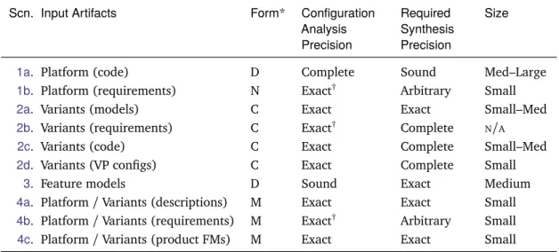
that consists of (1) a set of features; and (2) valid feature combinations, represented as feature dependencies or configurations; and (3) any supplemental information used to help with the tree or group recovery. Whether dependencies or configurations are recovered depends on the type of input artifacts (Table3.1). For example, dependen-cies can be recovered from a variable artifact, while a set of configurations is more appropriately recovered from a set of variants.

We separate the input artifacts of a variability-rich software project into the six cate-gories in Table3.1. The input artifacts are classified in terms of their level of abstraction by the columns. The rows describe whether the artifact is avariable artifactwhere vari-ability is symbolically represented in the artifact, or enumerated as aa set of instances. We borrow terminology from the Common Variability Language (CVL) to distinguish an artifact’s level of abstraction[Obj12]. An artifact that is avariability abstractionis at a high level of abstraction and contains concepts such as features[KCH+90]—properties that are relevant to some stakeholder[CE00]—or decision[SRG11]. An artifact is a

variability realizationif it describes how variability is realized or implemented in the system.

Different input artifacts require different forms of variability analysis. For exam-ple, given a set of requirements documents, where each document realizes a single variant [WCR09, NE08a], the analysis would involve analyzing each requirements document to extract features that are described in each. In another example, extracting

variability from source code requires a form of code analysis such as TypeChef for C preprocessor annotated code[Käs10]. Berger et al. developed analyses for analyzing FreeBSD configuration templates and mining dependencies from its build system and documentation[BSL+10a]. A set of feature configurations could also be used directly as input to the algorithm, e.g., hardware configurations in FreeBSD. Our work focuses solely on feature model synthesis and relies on existing work to perform the variability analysis stage.

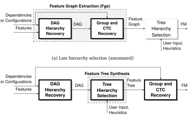
Feature Model Synthesis The stage following variability analysis, feature model synthesis, is responsible for building a feature model given the extracted abstract input. We decompose feature model synthesis into three stages (Figure3.3): (1) DAG hierarchy recovery, (2) group and cross-tree constraint (CTC) recovery, and (3) tree hierarchy selection. DAG hierarchy recoverytakes a set of features and a formula, and recovers a DAG that describe all hierarchies that imply the input formula. Group and CTC recovery identifies all feature groups and cross-tree constraints (CTCs) given the propositional formula, DAG and an optional tree hierarchy. Both the DAG hierarchy recovery, and the Group and CTC recovery stages are fully automated; no user input is required. Finally, since the hierarchy of feature models is a tree, thetree hierarchy selectionstage selects a single tree from the set of possible trees from the DAG. Both DAG hierarchy and group and CTC recovery are fully automated steps; only tree hierarchy selection may need user input.

The tree hierarchy selection stage selects a distinct tree hierarchy from the possible hierarchies that describe the same set of configurations. We demonstrate why this stage is needed with the input in Figure3.2a. The input describe three legal configurations as a disjunctive normal form (DNF) formula. The feature diagrams in Figure3.2band Figure3.2cboth describe the same input configurations. However, the meaning of the features are different depending on the selected hierarchy. In Figure3.2b,dst, which

Variability Abstraction Abstraction-Realization Interface Variability Realization Variable Artifacts

Feature model VPs and feature-to-VP mapping

Configurable platform requirements, models, code, etc.

Instances Feature configurations

VP configurations Variants

requirements, models, code, etc.