______________________________________________________________________________
An Evolutionary Transportation Planning Model:
Structure and Application
by David M. Levinson
submitted to Transportation Research Board July 9, 1994
revised November 30, 1994 final revision April 20, 1995
shortened May 22, 1995
published Transportation Research Record #1493 p. 64-73
Abstract
This paper describes an evolutionary transportation planning model wherein the demand in a given year depends on the demand of the previous year. The model redistributes a fraction of the work trips each year due to the relocation of a household or taking a new job, while changes in distribution due to growth (or decline) are considered. This hybrid-evolutionary model is compared with an equilibrium model, wherein supply and demand are solved simultaneously. The reasons for preferring the evolutionary method to the equilibrium approach are several: (a) the ability to more easily use observed data and thereby limit modeling to changes in behavior; (b) additional realism in the concept of the model; (c) the provision of a framework for extension to integration with land use models; and (d) the additional information available to policy makers .
Introduction
Traditionally, transportation planning models are used to forecast levels of traffic or transit ridership at a given point in time. Best practice in travel forecasting, the equilibrium approach, attempts to simultaneously (or iteratively) solve for travel demand given a congested network and to estimate network congestion given the travel demand. However, at no point in time is the demand/supply system actually in perfect equilibrium. Individuals and firms continuously enter and leave the system. Changes in system performance, such as the travel times between places, lead further changes in user behavior, such as choice of route, mode, departure time, sequence of trips, or destination. Some of these behavioral changes are made readily with only a short lag. The disruptive nature and high transaction costs of others, such as switching jobs or moving to a new residence, mean they are undertaken rarely.
This paper presents and tests an alternative approach to travel demand modeling which explicitly considers changes over time in work trip distribution as a result of household
relocation and job switching. The behavioral theory underlying this model is not the perfect network equilibrium of Wardrop or the supply/demand equilibrium described by Boyce and others ( 1 ). Rather, it is comparable to Simon’s idea of bounded rationality, where the costs of changing behavior need to be considered as well as the possible sub-optimality of that behavior ( 2 ). Thus, supply and demand are not in perfect equilibrium because the costs of moving and switching jobs is high. Traffic assignment may not be in perfect equilibrium because individuals do not have perfect information about the dynamically changing travel times between places.
The approach presented here is therefore more analogous to an evolutionary model than an equilibrium model. The dichotomy and connection between the two have been long
recognized ( 3 ). In a strictly evolutionary model, decisions are updated continuously (or in more practical terms on some time slice such as a day-to-day basis), with some time lag between obtaining information and executing a change in behavior. Moreover, the time lag for response may vary based on the type of decision and the characteristics of the individual making the decision. In this paper’s hybrid-evolutionary model, day-to-day decisions are still treated as
______________________________________________________________________________ though they are in equilibrium, but long-term decisions are lagged. In this case, only a fraction of work trips are re-distributed every year, with congested travel times based on the previous year's results serving as the source of impedance. In addition, trips from new homes and jobs are also distributed based on those times. One key question is: To what extent do different travel patterns emerge from the evolutionary modeling approach compared with an equilibrium approach?
In addition to being more realistic, one advantage to the evolutionary approach is the ability to start with observed data such as the Census Journey to Work data or a trip table
synthesized from traffic counts and an old trip table. The evolutionary approach (in this paper, a synthesized trip table is used as a seed) can begin with all of the information inherent in these data rather than just the impedance curves derived from them, and evolve incrementally from observed conditions rather than be modeled in totality. This approach is expected to be better than simply applying zone-to-zone adjustment factors at the end of the equilibrium modeling process to correct demand for under or over-estimation because it reduces the amount of error introduced by modeling.
The evolutionary approach should also have significant advantages for future application to land use forecasting and combined transportation-land use forecasts. While the transportation model is a largely negative feedback loop: More demand creates more congestion which leads to less demand; the land use model is in some respects a positive feedback loop: More
development increases accessibility which leads to more development. At the extremes, positive feedback leads to the densities found in Manhattan or Hong Kong. The integration of positive and negative feedback results in a complex model that is more sensitive to historical patterns and initial conditions than a simpler equilibrium-seeking negative feedback loop. However, the model presented in this paper considers land use changes as exogenous for two reasons: (1) the lack of resources to calibrate a land use model to the necessary accuracy, and (2) the lack of support for computer modeling of land use, planners in the Washington D.C. area prefer a hand-crafted approach using Delphi methods for forecasting land use.
Further, many policy decisions, such as the programming of capital facilities, are made by analysis of a single, equilibrium point in time. A evolutionary model can measure the transportation system over multiple time slices and give a more accurate reflection of benefits and costs.
The largest drawback to the evolutionary approach is the additional computational time required to implement the system as opposed to a one-shot equilibrium solution. If the results are not sufficiently different, or the additional information is not useful, the benefit may not be worth the additional computer resources and complexity. A second consideration is the requirement for additional information. In an evolutionary model, the different time lags in decision-making must be determined. In this case: How frequently do individuals relocate? Here, a fixed value of 22.5 percent of individuals are taken to change jobs, houses, or both every year, a figure derived from the 1991 Montgomery County Travel Survey ( 4 ), but future research should model the value endogenously based on socio-economic, demographic, and
transportation accessibility variables for a given area or trip interchange.
Next in this paper is a discussion of model structure. This includes frameworks for modeling travel demand, a model of relocation behavior, and flowcharts of the hybrid-evolutionary and equilibrium models. This is followed by a description of the model
components used in this application. The model inputs of land use, demographics, and networks are presented. A comparison of the convergence properties of the two models is shown. A section comparing the results of the two models is provided. The conclusion discusses some of the questions raised by the evolutionary model.
Model Structure
This section discusses the model structure presented here. First is a look at modeling
frameworks, considering equilibrium and evolution as two poles with two interim combinations of the methods depending on the decision time horizon evaluated. Next is a presentation of how relocation is incorporated into the model system mechanically. Finally is a comparison of flowcharts of the two tested models: hybrid-evolutionary and equilibrium.
______________________________________________________________________________
Travel Demand Modeling Frameworks
Several approaches can be taken in testing the concept of a dynamic demand model. Each approach is a variation on the spectrum between a lagged model, where decisions are not simultaneously made by all commuters, and an equilibrium model. In the aggregate models tested here, it is assumed that there are two time frames for travel decisions: day-to-day and year-to-year. Day-to-day decisions include route choice, mode choice, departure time choice, and non-work trip destination choice. Year-to-year decisions include relocation or work trip (re-)distribution (for a fraction of commuters), auto ownership, and trip (re-)generation. These decisions are not entirely separable, so endogenous year-to-year decisions (location/ work trip distribution) reflect changes in the day-to-day conditions. In addition, the following system variables vary on an annual basis: network , land use, demographics. While there is a continuum of decision making in reality , this approach is taken for the sake of simplicity.
Further it is assumed that year-to-year decisions are lagged, based on information from the previous year, but that day-to-day decisions are essentially in equilibrium between demand and supply.
The models are as follows:
Model 1. Equilibrium:Equilibrium for Day-to-Day and Year-to-Year
Model 2. Hybrid: Equilibrium for Day-to-Day, Evolution for Year-to-Year Model 3. Evolutionary: Evolution for Day-to-Day and Year-to-Year
Model 4. Alt. Hybrid: Evolution for Day-to-Day, Equilibrium for Year-to-Year
Because of computational intensity (3652 days for 10 years, requiring a demand update on each day), Model 3 is not pursued here. In addition, Model 3 would need to account for variations in demand due to day-of-week and month-of-year. Model 4, an alternative hybrid model, would use dynamic assignment, scheduling, and departure time, perhaps with responsive intersection control, to come up with information used in long term decisions, which would be assumed to be in equilibrium, and is the opposite of Model 2. In all of Model 2 runs here , the yearly decisions (trip generation, work trip distribution, auto ownership) are computed as lagged decisions.
Relocation
For an evolutionary analysis, a new model component is required. This concerns the decision to relocate: both moving one’s home or switching jobs is a relocation decision. Here, the terms relocate and redistribute are considered synonymous, the difference in terms resulting from alternative perspectives: individuals choose to relocate while social planners redistribute individuals (match their home and workplace) in their demand models. The nature of this model is that the number of trips at time t depends on the trip pattern at time t-1 plus any change
forecast to happen. This is an inertial, state-dependent approach, a work trip does not change from year to year unless some outside force (a redistribution/relocation decision) causes it to change. On a much longer time scale, long-term location (and hence trip frequency/destination choice) decisions can be seen as analogous to trip chaining, where decisions are history
dependent. Kitamura has shown for trip chaining that the use of lagged dependent variables is a plausible and statistically valid specification ( 5 ). Clearly, empirical and statistical issues will need to be further investigated for relocation choice to determine the best specification in terms of predictive value while avoiding serial correlation problems.
This model needs to re-match a fraction of all workers and jobs into work trips for each time slice (in this case, each year). Further study is necessary to understand whether these recently redistributed trips are of longer, shorter, or the same duration as average trips after controlling for the number of opportunities and competing job seekers. This question is analogous to the difference between marginal and average costs in economics. In this application, the work trip distribution impedance curves were estimated from the a survey sample of the entire population (not only those who recently moved).
The following equations are used:
Tijy = (1-Rij) x Tijy-1 + MNijy (1) where: Tijy = Trips from i to j in year = y
MNijy = Switched Job/House and New Trips (subject to redistribution) Miy = Trips from i in year y which switched from year = y-1
______________________________________________________________________________ Mjy = Trips to j in year y which switched from year = y-1
Niy = Trips from i due to growth (not present in year = y-1) Njy = Trips to j due to growth (not present in year = y-1)
Rij = Relocation function for interchange i-j (=0.225 in this application) subject to J Tiy =
∑
Tijy (2) j=1 I Tjy =∑
Tijy (3) i=1 Miy = Rij Tijy-1 (4) Mjy = Rij Tijy-1 (5)For work trip distribution, a two-dimensional balancing procedure is used. For this, the rows (origins) and columns (destinations) are balanced. The total of origins (Oiy) balanced here is:
Oiy = Niy + Miy (6)
and the destinations (Djy) is:
Djy = Njy + Mjy (7)
which after balancing, produces the trip table MNijy, which is added to the fraction of trips unchanged from the previous year to obtain the final peak period work trip table.
The following table shows the logic of whether an individual would be redistributed:
Change Work Location
Yes No
Change Yes Redistribute Redistribute
Flowcharts
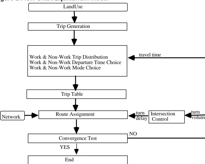
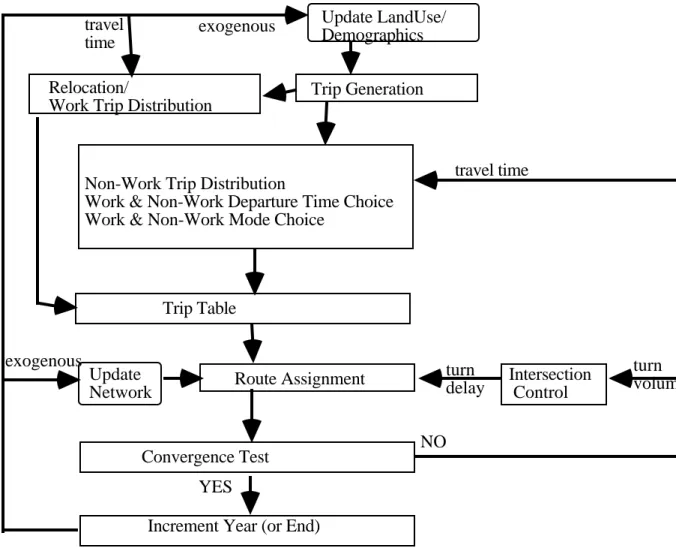
Figures 1 and 2 show the flow chart of the equilibrium and hybrid-evolutionary models respectively. The endogenous components are identified with rectangles, the exogenous updates to land use and networks are shown with curved corners.
To summarize, exogenous changes over time in the model include updates to the transportation network through the addition of links, updates of the age distribution and
household size distribution by geographical area developed from a separate demographics model, and updates of the land use activity (housing units and employment by type) from regional transportation forecasts. These are discussed in detail in a later section. Collectively, these inputs are treated exogenously, because in the short term, there is little interaction between them and travel demand. The longer the timeframe, the more that can reasonably be internalized.
Endogenous changes within this model include updates to travel times on the network, the number of work trips generated, and consequently the interchange of work trips between zones, and in a more complete extension of the proposed model, the relocation decision. Travel demand is not limited to just trips generated, but considers all of the choices in the travel demand process. Therefore, a shift in mode, route, or time-of-day is a change in demand for a facility or route just as an increase or decrease in the number of trips generated is a change the demand for the transportation system as a whole.
Model Components
The model components (trip generation, trip distribution, mode choice, departure time choice, route choice, and intersection control) used here are the same as those estimated for the Travel/2 model ( 6 ). Briefly, these are described below.
Trip Generation
The person trip generation model is two parts ( 7 ). For the home end of trips, a cross-classification model based on age, household size, and dwelling unit type. For the non-home end, generation is based on number of employees (office, retail, industrial, other). The purposes
______________________________________________________________________________ used in the model are: Work to Home, Work to Other (to Home), Home to Other, Other to Home, Other to Other, Home to Work. Trip generation is computed for the afternoon peak period (3:30 - 6:30). In the hybrid model discussed in this paper, both Work to Home and Work to Other (to Home) purposes are considered “work trips”, the other purposes are considered “work”. As this is a person-trip model, mode choice is estimated for both work and non-work trips, and all modes (including non-motorized). Future research should derive trip generation from a activity approach considering activity frequency, duration, and scheduling.
Destination Choice
A multi-modal trip distribution model is used in this model ( 8 ). A composite impedance calculated as the weighted average of the mode-specific impedances is computed, using mode shares as the weight. In the hybrid model, for non-work trips, destination choice is computed in equilibrium with route assignment and intersection control. For all relocated and new work trips, the final travel times from the previous year are used to compute the trip distribution in the subsequent year. Other trips are carried from the previous year. Detailed information on the estimation of the initial (seed) trip table is available from the author, and was not included for reasons of space.
Departure Time Choice
Departure time choice determines the proportion of peak period vehicle trips which occur in the peak hour. It is a binomial logit model with two choices: peak hour and not peak hour. The factor which is used to determine probability of peak hour is the ratio of congested to freeflow time on a zone-interchange basis. This component is solved in equilibrium with route assignment and intersection control for both work and non-work trips.
Mode Choice
In this application of the model, mode choice is held fixed at 1990 levels. Earlier tests of the model found little differentiation of mode choice due to the changes in network and land use between 1990 and 2000 when policies are kept fixed. In theory, this component could be solved in equilibrium with route assignment and intersection control. However, to reduce computational
time and possible sources of minor variation, the zone-to-zone mode shares were therefore kept constant. Future research should consider a simultaneous approach to mode and departure time choice, and possibly destination choice, at least for non-work activities. Though various
questions about the relative timing of these components would need to be resolved.
Route Choice and Intersection Control
A single-class user equilibrium assignment model provided by the EMME/2 software is used in this application ( 9 ). This model considers both link delay and turn delay. The inputs to turn delay (cycle length, green time per phase) are computed with an external program each iteration of the auto assignment, and the results are fed back into the turn penalty function ( 6 ).
Exogenous Model Inputs
Two key sets of exogenous data are used in the model: land use and demographic changes by zone, and modifications in the highway and transit networks. These are described in turn below.
Land Use and Demographics
The land use assumptions in this application are derived from the Round IV forecasts of the Metropolitan Washington Council of Governments and the Round IV forecast of the
Baltimore Regional Council of Governments ( 10-11 ). In 1990, for Montgomery County, Maryland, the focus of this study, the number of housing units was 280,000 and jobs was 460,000 , which is expected to increase to 320,000 housing units and 580,000 jobs by 2000. These forecasts are based in large part on approved but unbuilt development (typically a six to twelve year inventory) and by the queue of development which is applying for development approval. Future land use forecasts will incorporate estimates of transportation accessibility explicitly, and perhaps eventually the forecasting will be integrated. However, as noted earlier, resistance to combined transportation/land use forecasting in the Washington area is at least as political as technical. Demographic inputs (age distribution by area, average household size) are updated each year based on results from an exogenous demographic forecasting process
______________________________________________________________________________
Networks
A dynamic model requires that changes to the transportation network be coded to the year of change. Here, the model transportation networks come from the Montgomery County
Planning Department (for Montgomery County), the Metropolitan Washington Council of Governments (for the rest of metropolitan Washington) and the Baltimore Regional Council of Governments (for metropolitan Baltimore). The future network within Montgomery County has coded changes in link capacities (number of lanes) as well as additional links to the year of opening. Outside Montgomery County, the change in networks occur for the base year and 1995. Thus the capacity outside Montgomery County from 1990 to 1995 and from 1996 to 2000 is fixed.
Model Convergence
Figures 4 and 5 show convergence results for the two models, both in the year 2000 time horizon summarizing the entire model region. The results for the equilibrium model represents the value of the objective function on each iteration in year 2000. The results for the hybrid-evolution model reflect the decisions decided in equilibrium (non-work trip distribution, time-of-day choice, and route choice) also in year 2000 for each iteration. In the evolutionary model, there is no convergence from year to year (as discussed in the next section on results). Figure 4 shows the Total Vehicles on the Network, which for both runs converges to about 1 million vehicles by the 30th iteration. The equilibrium model has somewhat more vehicles than the hybrid-evolution model, although more research will be necessary to say whether this is inherent in the model structure or just an artifact of the particular data set. It should be noted that the
Hybrid-Evolutionary model converges more quickly than the Equilibrium model, probably because one major component, work trip distribution, is fixed before the model is run for a given year. By the 10th iteration the Hybrid model has a demand that is substantially identical to the 30th iteration, however it takes 15 iterations for the same to be true of the equilibrium model.
Figure 5 shows the convergence of the objective function (absolute gap) for the two models. The gap is an estimate provided by the EMME/2 software of the difference between the
current assignment and a perfect equilibrium assignment in which all routes used for a given OD pair would have the same length ( 9 ). The value is tending to level out at about 1 million by the 25th iteration.
Thus, for any given time slice (one year), the hybrid-evolutionary model reaches an equilibrium, although over time, the equilibrium point moves. This particular structure, which is largely composed of convergent negative feedback loops is unlikely to have the potential for chaos, cascades, or catastrophes. However, depending on the rate of change of exogenous variables such as the network description or amount of development, the equilibrium point should move more or less smoothly.
Results
Some summary figures are provided for the various models to compare their results. Figure 6 shows the peak hour vehicle trips (the same result as in figure 4) for each year, again for the entire model region. The number of trips tends upward in the Hybrid model, but is less than the Equilibrium model. The large uptick in 1995 is due to the increased network capacity which is coded to come on line in that year (recall that outside Montgomery, capacity from 1990 to 1994 is the same, as it is from 1995 to 2000.) This clearly emphasizes the need for time coding of networks if this approach is to be used.
Figure 7 shows the Vehicle Miles Traveled within Montgomery County for the two models. Again the Hybrid model is somewhat less traveled than the Equilibrium model. VMT shows a sharp increase from 1990 to 1991. In that year I-270 was widened from 6 to 12 lanes through much of the county, which resulted in increased demand. Otherwise the growth is fairly smooth.
Figure 8 displays the average work trip time (in minutes), length (in kilometers), and speed (in kilometers per hour) for Montgomery County work trip origins (since this is the afternoon, origins are Montgomery County workers going home). All three values are stable across the decade, indicating that the feedback process is maintaining these attributes. In fact, speed improves over this period while travel time decreases slightly, indicating appropriate
______________________________________________________________________________ capacity increases and shifting travel patterns to suburb-suburb trips, which have higher average speeds. Difference of means tests performed over the ten years, comparing the mean traffic zone time and speed (comparing 1990 and 2000 results for the model) show that the results for year 2000 are statistically different from those in 1990 for the hybrid-evolutionary model for time and speed, but the same for length. For the equilibrium model, the time, speed, and length did not show a statistical difference.
Figure 9 shows the proportion of Montgomery County links in each level of service category (LOS A - F). No trend is apparent . In fact for the year 2000, the percentage of links better than LOS C/D is identical in both the Hybrid and Equilibrium models. Figure 10 shows the intersection LOS (using the critical lane volume method) for intersections in the county. Again no trend is apparent, and the number of intersections above LOS C/D in both models is the same in the year 2000.
Conclusions
This paper discusses some of the implications of introducing dynamic work trip demand into the transportation planning model. As a behavioral assumption for the forecasting of a specific year in the mid-term, evolution is conceptually better than equilibrium. The results were similar, but not identical between the two models. The length of the time period under study and the relative change in input data may influence model results.
The question of equilibrium or evolution is important in the context of attempts to construct dynamic models of urban structure and growth or travel demand. Most such large scale models are now static, or dynamic in only the crudest sense, using five year time slices ( 12 ). However, the structure and function of every city, and the behavior of individuals within that city, depend crucially upon their mutual co-evolutionary history. Because cities and human activity patterns evolve through time in complex, dynamic “environments”, the interactions of urban form and human behavior do not, and should not be expected to, conform to equilibrium conditions. As Forrester says “The urban system is a complex interlocking network of positive
and negative feedback loops. Equilibrium is a condition wherein growth in the positive loops has been arrested.” ( 13 ).
The reasons for preferring the evolutionary method to the equilibrium approach are several: (a) the ability to fully incorporate an observed data set such as a vehicle (or transit) trip table synthesized from traffic counts ( 14 ) (or transit ridership data) and the Census Journey to Work data, unlike the use of equations and adjustment factors, all of the information inherent in the observed data can be used, and only the change over time needs to be modeled; (b) additional realism in the concept of the model; (c) the provision of a framework for extension to integration with land use models; (d) the additional information available to policy makers for decisions such as the sequence of programming and constructing capital facilities, where the benefit depends on the timing of the facility.
This research points out the need to develop realistic behavioral models of switching in all model components. For instance the Wardrop equilibrium principal states that no route is used between an O-D pair if the travel time is greater than on another route. But this implies perfect information. Once individuals have selected routes, their travel times change from day to day for a variety of factors. At what point does an individual decide to try another route? Under what conditions will this commuter stay with the second route or return to the first? How will Advanced Traveler Information Systems play into this? Switching is an issue in departure time choice, activity sequencing, mode choice, and non-work trip destination selection (e.g. the choice of a grocery store). These and other questions will need to be answered as dynamic
evolutionary modeling is implemented.
Some practical issues also emerge. There are not yet enough data to know the long term temporal stability of this relocation value. What is it a function of? Are distribution curves (and other components) the same at the margins as they are on average? Further research can be aimed at implementing a full day-to-day evolutionary travel/activity demand simulation, with models of switching rather than attempting to predict the behavior of the entire population.
______________________________________________________________________________ However, in the near term, application of supply/demand equilibrium models of travel demand is still preferable to conventional application with fixed zone-to-zone travel times independent of changes in the transportation network.
References
1. Boyce D.E. , LeBlanc L., and Chon K. Network Equilibruim Models of Urban Location and Travel Choices: A Retrospective Survey Journal of Regional Science , Vol. 28, No 2, 1988 2. Simon, H. (1955) A Behavioral Model of Rational Choice Quarterly Journal of Economics 69,
pp. 99-118
3. Harris, Britton. 1970. “Change and Equilibrium in the Urban System”, Highway Research
Record #309, p.24-33.
4. Kumar, Ajay. and Replogle, M. 1992 Low-Cost Travel Panel Survey presented at First U.S. Conference for Panels for Transportation Planning, Lake Arrowhead, California Oct 25-27, 1992
5. Kitamura, Ryuichi. 1987. “Sequential, History-Dependent Approach to Trip-Chaining Behavior”, Transportation Research Record # 944 p13-22
6. Levinson, David and Kumar, Ajay. 1994. Integrating Feedback into the Transportation Planning Model: Structure and Application , Transportation Research Record 1413, Transportation Research Board
7. Levinson, David and Kumar, Ajay. 1994. Specifying, Estimating, and Validating a New Trip Generation Structure: A Case Study of Montgomery County Maryland , Transportation
Research Record 1413, Transportation Research Board
8. Levinson, David and Kumar, Ajay. 1995. A Multimodal Trip Distribution Model: Structure and Application . Transportation Research Record #1466, p 124-31
9. INRO. 1993 EMME/2 User’s Manual: Release 6 Montreal, Canada
10. Metropolitan Washington Council of Governments 1989. "Round IV Cooperative Forecast", Washington, DC
11. Metropolitan Baltimore Council of Governments. 1991. "Round IV Cooperative Forecast", Baltimore MD
12. Wegener, M. 1994 Operational Urban Models: State of the Art. Journal of the American
Planning Association 60,1: 17-30.
13. Forrester, Jay. 1969. Urban Dynamics. Cambridge, MA: MIT Press p. 121
14. Spiess, H. 1990 A Gradient Approach for the O-D Matrix Adjustment Problem Center for Transportation Research Paper #692, University of Montreal, Montreal Canada
Acknowledgements
The author would like to thank Chris Winters, Ajay Kumar, David Gillen and three anonymous reviewers for their review of earlier draft sof this paper. The author would also like to
acknowledge the help of the Univeristy of California at Berkeley, and the Montgomery County, MD Planning Department. The opinions expressed in this paper are the responsibility of the author.
______________________________________________________________________________
Figure 1 Flow Chart Equilibrium Model
LandUse Trip Generation Route Assignment Convergence Test End Intersection Control NO YES Trip Table
Work & Non-Work Trip Distribution Work & Non-Work Departure Time Choice Work & Non-Work Mode Choice
Network travel time turn volume turn delay
Figure 2: Flow Chart Hybrid Evolutionary Model
Update LandUse/ Demographics Trip Generation Relocation/
Work Trip Distribution
Route Assignment
Convergence Test
Increment Year (or End)
Intersection Control NO
YES Trip Table Non-Work Trip Distribution
Work & Non-Work Departure Time Choice Work & Non-Work Mode Choice
Update Network travel time turn volume travel time exogenous exogenous turn delay
1990 1991 1992 1993 1994 1995 1996 1997 1998 1999 2000 Year 250 300 350 400 450 500 550 600 Thousands
Units (houses, jobs)
Houses Jobs
1 2 3 4 5 6 7 8 9 1 0 1 1 1 2 1 3 1 4 1 5 1 6 1 7 1 8 1 9 2 0 2 1 2 2 2 3 2 4 2 5 2 6 2 7 2 8 2 9 3 0 Iteration 800 1000 1200 1400 1600 1800 2000 2200 Thousands
Total Vehicles on Network
Hybrid-Evolution Equilibrium
note: see text for description
1 2 3 4 5 6 7 8 9 10 11 12 13 14 15 16 17 18 19 20 21 22 23 24 25 26 27 28 29 30 Iteration 100000 1000000 10000000 100000000 1000000000 10000000000 100000000000 1000000000000
Absolute Gap (Assignment Objective Function)
Hybrid-Evolution Equilibrium
note: see text for description
1990 1991 1992 1993 1994 1995 1996 1997 1998 1999 2000 Year 960 970 980 990 1000 1010 1020 Thousands Total Vehicles Hybrid-Evolution Equilibrium
Entire Model Region
1990 1991 1992 1993 1994 1995 1996 1997 1998 1999 2000 Year 1620 1640 1660 1680 1700 1720 1740 1760 Thousands
Vehicle Miles Travelled
Hybrid-Equilibrium Equilibrium
Montgomery Co. Links
1990 1991 1992 1993 1994 1995 1996 1997 1998 1999 2000 Year 15 20 25 30 35 40
Units (kilometers, minutes, kph)
Length - Hybrid-Evolution Length - Equilibrium Time - Hybrid-Evolution Time - Equilibrium Speed - Hybrid-Evolution Speed - Equilibrium
Montgomery County Work Trip Origins
1990 1991 1992 1993 1994 1995 1996 1997 1998 1999 2000 EQUILIBRIUM 2000 Year 0 0.2 0.4 0.6 0.8 1 Proportion A B C D E F
Montgomery Co. Links
1990 1991 1992 1993 1994 1995 1996 1997 1998 1999 2000 EQUILIBRIUM 2000 Year 0 0.2 0.4 0.6 0.8 1 Proportion A B C D E F
Montgomery Co. Intersections