MATRIX COMPLETION OF NOISY GRAPH
SIGNALS VIA PROXIMAL GRADIENT
MINIMIZATION
Pere Gim´enez-Febrer, Alba Pag`es-Zamora
SPCOM Group, Universitat Polit`ecnica de Catalunya-Barcelona Tech, Spain
Abstract—This paper takes on the problem of recovering the missing entries of an incomplete matrix, which is known as matrix completion, when the columns of the matrix are signals that lie on a graph and the available observations are noisy. We solve a version of the problem regularized with the Laplacian quadratic form by means of the proximal gradient method, and derive theoretical bounds on the recovery error. Moreover, in order to speed up the convergence of the proximal gradient, we propose an initialization method that utilizes the structural information contained in the Laplacian matrix of the graph.
Index Terms—matrix completion, signal processing on graphs, proximal gradient
I. INTRODUCTION
In [1], Cand`es and Retch formulated the matrix completion problem as a convex minimization of the nuclear norm of the partially observed matrix, and demonstrated that an exact recovery of the original matrix is possible whenever the matrix is low rank, incoherent and uniformly sampled. The same framework is used in [2] for the recovery from noisy observations. The assumptions made imply that the matrix entries are unstructured, which is usually not the case for real data. Therefore, some works have extended the work in [1] by including extra information about hidden matrix structures into the problem formulation. For instance, in [3] an additional restriction is imposed so that the columns of the recovered matrix are a linear combination of the basis elements in a dictionary. In [4], it is observed that the temperature measure-ments taken by the sensors in a wireless sensor network are temporally stable in the short term, so a regularization term is added to ensure the short term stability of the recovered data. In the problem of predicting an incomplete matrix of ratings in [5], groups of users with similar background are assumed to have similar preferences, thus a penalty term is included to reduce the variability of the predicted ratings within a group. An alternative approach to capture the interdependence between the entries in the matrix is by applying techniques from the field of signal processing on graphs. As described in [6], [7], this field extends classical signal processing tools such as filtering or domain transformations and applies them to signals on a graph, so that the vertices in the graph measure signals and the graph edges model the underlying This work has been funded by the “Ministerio de Econom ıa y Com-petitividad” of the Spanish Government, ERDF funds (TEC2013-41315-R,TEC2015-69648-REDC,TEC2016-75067-C4-2-R) and the Catalan Govern-ment (2014 SGR 60 AGAUR).
relational structure of those signals. The connections between the vertices are represented by the weighted adjacency matrix of the graph, which can be known beforehand or inferred from the data as, for instance, in [8]. With regards to the matrix completion problem, so far the existing works under the signal processing on graphs perspective take advantage of the fact that the graph signals are known to be smooth on a given graph. For instance, in [9] the signals are assumed to be smooth on a graph when the data from connected vertices have similar values. Hence, the Laplacian quadratic form is added as a regularization function to the problem in [1] to enforce this smoothness on the recovered data. Additionally, a function named total variation is used in [10] as a regularization term to enforce the graph structure described by the adjacency matrix. Similarly, [11] takes on the collaborative filtering problem assuming that the original matrix can be factorized into two smaller matrices which lie on two different graphs.
In this paper, we focus on the recovery of partially observed graph signals that are arranged in a data matrix when the observations are noisy. We solve the problem by adding the Laplacian quadratic form as a regularization term as in [9], [11], and using the proximal gradient (PG) method, which allows us to derive theoretical bounds on the recovery error and give insight into the effect of the regularization. Moreover, we also propose an initialization method to reduce the number of iterations required to reach a solution. The remaining of this paper is organized as follows. Section II introduces the matrix completion problem, the PG algorithm, and the proposed initialization method. Section III analyzes the recovery error of the PG. Finally, Section IV includes the simulation results.
II. MATRIX COMPLETION FOR GRAPH SIGNALS Consider the undirected weighted graph G = (V,E,A), whereV ={v1, . . . , vN} is the set of vertices,E ⊆ V × V is
the set of edges connecting the vertices, and A∈ RN×N is
the weighted adjacency matrix. This matrix is defined so that a non-zero entry Ai,j indicates that information flows from vertex j to vertex i, and the magnitude of the entries is a measure of similarity or dependence between the connected vertices. GivenG, a graph signal is defined as a map from the set of V vertices into a set of real numbers y : V →R that
can be arranged in a column vectory defined as
wherey(i)is the value of the signal at vertexvi.
Consider now a set of graph signals {yl, ∀l = 1, . . . , L}
residing on the graph G, and let Y be the N×L matrix of graph signals
Y = [y1, . . . ,yL].
MatrixY is assumed low rank and cannot be observed except for a subset Ω ⊂ {1, . . . , N} × {1, . . . , L} of entries, which are corrupted by noise so that the matrix of observed entries
M ∈RN×L is defined as Mi,j=
(
Yi,j+∆i,j, when(i, j)∈Ω,
0, when(i, j)6∈Ω,
where ∆ is a sparse noise matrix with nonzero entries ∆i,j∀(i, j)∈Ω. For convenience, we also define the
com-plement subset of ΩasΩc, the cardinality of a subset as | · |, and the operator (·)Ω which projects a matrix X onto the subset Ωas follows
(XΩ)i,j= (
Xi,j, when (i, j)∈Ω,
0, when (i, j)6∈Ω.
Thus, our objective is to recover the original matrix Y from the observed noisy entries inM.
According to [2], one can recover Y with an error propor-tional to the noise by solving the following convex optimiza-tion problem: ˆ Y = argmin X ||X||∗ (1) subject to XΩ−M F≤ ||∆||F
where ||·||∗ denotes the nuclear norm defined by ||X||∗ =
Pr
i=1σi, with σi being the singular values of X and r its
rank, and ||·||Fis the Frobenius norm.
We can reduce the impact of the noise and take advantage of the structural information provided by the graph by incorporat-ing its Laplacian matrix into the matrix completion problem. The quadratic Laplacian form measures the smoothness of a signal on the graph and is defined as
L(X) =Tr(XTLX) =XL
l=1
X
(i,j)∈EAi,j(Xi,l−Xj,l) 2, where L =diag(A1)−A is the Laplacian matrix, 1 is the all-ones vector, and Tr(·) denotes the matrix trace operation. The matrix completion problem is commonly [10], [12], [13] solved by minimizing the Lagrangian form of (1) as
argmin X 1 2 XΩ−M 2 F+β||X||∗+αL(X), (2) where the nuclear norm becomes a regularization term with regularization parameter β, and we have incorporated the Laplacian quadratic form as an additional term weighted by a parameterαin order to promote similarity between the edges connected on the graph.
Proximal gradient is a popular method to solve nonsmooth optimization problems such as (2) thanks to its ease of implementation, and the good results it offers [10]. As proven in [14], the solution to (2) is given by the following iterative
scheme which performs a proximal gradient minimization for k≥1:
Xk=Stβ(Xk−1−t(XkΩ−1−M+ 2αLXk−1)). (3) The parametertis the step size of the gradient, andStβ(·)is
the matrix shrinkage operator (MSO), which, given the singu-lar value decomposition (SVD) of a matrixXasX=UΣV, we define as
Stβ(X) =U(Σ−tBX)V.
The symbolBX denotes a diagonal N×Lmatrix with main diagonal bX = [β, . . . , β, σd t , . . . , σD t ],
where D = min(N, L), and {σd, . . . , σD} are the singular
values of X smaller thantβ, that is, σi< tβ ∀i≥d.
A. Proximal gradient initialization
Algorithms for matrix completion are usually initialized to the observed matrixM, a low-rank approximation of M or a random matrix [15]. Here we propose to take advantage of the information provided by the Laplacian matrix to compute an initial point X0, hopefully closer to the optimal solution, that will reduce the number of iterations required by the PG algorithm to converge.
One of the properties of the Laplacian matrix is that its smallest eigenvalue has value 0 with multiplicity equal to the number of connected components on the graph. Let matrix L have eigenvalue decomposition L = QΛQT, and Q0 ∈ RN×P be the matrix containing the P eigenvectors
with associated eigenvalue 0. Indeed, Q0 contains the graph signals that are smoothest on the graph so that L(Q0) = 0. Thus, as the initial matrixX0, we propose to use matrix M and complete the zero entries using a weighted combination of the signals inQ0. Specifically, the initialization matrix is obtained as
X0= (Q0C0)Ω
c
+M, (4)
whereC0∈RP×Lis the matrix of coefficients that better fits
Q0C0 to the observed entries, that is,
C0= argmin
C
||M−(Q0C)Ω||2F. (5)
If we denote C0 = [c1, . . . ,cL], the problem in (5) is
equivalent to solving {c1, . . . ,cL}= argmin c1,...,cL L X l=1 ||ml¯ −SlQ0cl||22, (6)
where ml¯ is a vector of length el containing the observed samples of thelthcolumn ofM, andSlis ael×N sampling matrix. MatrixSlhas a single non-zero element per row equal to 1, and it is built so thatml¯ =Slml. The solution to (6) is
cl= (QT0SlTSlQ0)−1QT0S
T
l ml¯ ∀l= 1, . . . , L.
The computational cost of this initialization is O(N3)due to the eigendecomposition ofA, which is comparable to the cost of one PG iteration.
III. ERROR ANALYSIS
In this section we analyze the recovery error of the PG algorithm and how the addition of the Laplacian quadratic form as a regularization term impacts on the noise. Before introducing the main results, we first make and define the following assumption and lemmas:
Assumption 1. Similar to Assumption 7 in [13], we assume that, given small enoughαandt, there exists a constant0≤
γ<1such that for any matrix X (I−2αtL)X−tXΩ F≤γ||X||F.
Lemma 1. Given a pair of matricesX andZ,
||Stβ(X)−Stβ(Z)||F≤ ||X−Z||F. Proof. The proof of this lemma can be found in [14]. Lemma 2. For any matrixX
||Stβ((I−2αtL)X)−X||F≤√rtβ+ 2αt||LX||F. (7)
Proof. We begin by showing that ||Stβ((I−2αtL)X)−X||F
=||Stβ((I−2αtL)X)−X+ 2αtLX−2αtLX||F ≤ ||Stβ((I−2αtL)X)−(I−2αtL)X||F+ 2αt||LX||F.
Next, let us define matrix X0 = (I −2αtL)X with SVD
X0=U0Σ0V0. Then,
||Stβ((I−2αtL)X)−X||F≤ ||Stβ(X0)−Stβ(X0+tβI)||F
+ 2αt||LX||F.
Finally, we apply Lemma 1 and obtain (7).
We now introduce the following theorem which bounds the recovery error of the original matrix when the observed entries are noiseless:
Theorem 1. Let Yˆ be the rank restimate obtained with (3) after the PG has converged, with a noiseless observed matrix YΩ. Then ˆ Y −Y F ≤ √ rtβ+ 2αt||LY||F 1−γ . Proof. Since f(X) = 12 XΩ−YΩ 2 F+αL(X) is convex
and continuously differentiable, the proximal gradient con-verges to a solution in the optimal solution set of (2) which is also a fixed point of (3) [12]. Hence, since Yˆ is a fixed point of (3), we have that ˆ Y −Y F= Stβ( ˆ Y −t(YˆΩ−YΩ+ 2αLYˆ))−Y F = Stβ((I−2αtL) ˆ Y−t(YˆΩ−YΩ))−Stβ((I−2αtL)Y) +Stβ((I−2αtL)Y)−Y||F. ≤ Stβ((I−2αtL) ˆ Y−t(YˆΩ−YΩ))−Stβ((I−2αtL)Y) F +||Stβ((I−2αtL)Y)−Y||F. Applying Lemma 1: ˆ Y −Y F≤ (I−2αtL)( ˆ Y −Y)−t(Yˆ −Y)Ω F +||Stβ((I−2αtL)Y)−Y||F.
Next, we apply Lemma 2 and Assumption 1 and obtain
ˆ Y −Y F≤γ ˆ Y −Y F+ √ rtβ+ 2αt||LY||F,
which leads to the error bound in Theorem 1.
Intuitively, Theorem 1 shows that the recovery error with noiseless observations can be reduced by setting a lower β, as it was anticipated in [16], as well as by choosing a graph on which the graph signals in Y are smooth. Nevertheless, whether the error can be driven to 0 by havingβ →0depends on the number of observed entries and their distribution, which is implicit through the constantγ.
In order to assess the effect of the regularization on the noise, let us switch to another perspective. In the signal processing on graphs theory [6], [7], matrix QT obtained
from the eigendecomposition ofL is referred to as the Graph Fourier Transform (GFT) matrix. The eigenvectors in Q can be viewed as frequencies on the graph, with the eigenvectors associated to the smaller eigenvalues corresponding to the lower frequencies, that is, signals that vary slowly on the graph. Given a vectorx, the productLx=QΛQTxprojects the vector onto the graph frequency domain ofL, scales the frequency coefficients by Λ, and projects the result back to the graph domain given by Q. Therefore, the result of Lx
is a highpass filtered version of the vector since the lowest frequency coefficients in QTx associated with the smallest
eigenvalue, which is equal to 0, are eliminated and the rest are scaled according toΛ. Then, we can introduce the following theorem:
Theorem 2. GivenI0=ΛΛ†, whereΛ†is the pseudoinverse
ofΛ, the frequency content ofYˆ on the nonzero frequencies of the graph is bounded as
I0Q TYˆ F≤ 1 2α Λ †QT(YΩ −YˆΩ) F (8) + Λ†QT∆ F+ Λ†QTU0BYˆ0V0) F , where matrices U0,V0 are the left and right singular vector matrices of
ˆ
Y0 =Yˆ −t(YˆΩ−M)−2αtLYˆ. (9)
Proof. Let matrixYˆ0 in (9) have SVDYˆ0 =U0Σ0V0. Given an estimate Yˆ, which is a fixed point of (3), we have that
Stβ(Yˆ0) =Yˆ. Expanding the MSO in this last expression we obtain
ˆ
Y0−tU0BYˆ0V0 =Yˆ.
Now, if we replaceYˆ0by its definition, substituteM =YΩ+ ∆ and rearrange the resulting equation, we have
2αLYˆ =YΩ−YˆΩ+∆−U0BYˆ0V0. (10)
Note that if we multiply the matrix LYˆ by Λ†QT we are left with a GFT matrix of the columns ofYˆ, containing only
the coefficients of the nonzero frequencies. Hence, multiplying both sides of (10) byˆQT we obtain the bound in (8).
Theorem 2 shows that the Laplacian regularization has a lowpass filtering effect on the solution since the right-hand side of (8) vanishes withα. Moreover, the second term on the right-hand side of (8) also shows the filtering effect on the noise ∆ since the coefficients of its GFT are multiplied by Λ†. If the noise is not smooth on the graph, that is, L(∆) is large and the GFT coefficients are concentrated around the higher frequencies, its contribution to the spectrum ofYˆ will be small.
IV. SIMULATION RESULTS
We have tested the PG algorithm for the Laplacian-regularized matrix completion problem on a real dataset of temperature measurements. The algorithm has been run until convergence over Nrea = 20 realizations with different percentages of observed samples, denoted byPs=
|Ω|
N·L·100.
The parameters of the PG are β = 200, which is set relative to the singular values of the observed dataset, t = 0.05 and
α={0,0.5}. As a performance metric, we use the normalized mean square error at iteration k
NMSEk= 1 Nrea Nrea X n ||Xkn−Y||2F ||Y||2F ,
where Xk(n) is the estimate of the complete matrix Y at iterationkand realizationn. The initial estimates{Xk(n)∀n} are calculated using (4).
The datasetY is a150×365matrix of temperature readings taken by 150 stations over 365 days in 2002 in the United States. The graph signals yl are the temperature values
mea-sured at each station. In order to obtain the weighted adjacency matrix A, first a graphG0 with unweighted adjacency matrix
P0 is generated as in [10] for the stations. In this graph, each station is a vertex and is connected to the 8 geographically closest stations. Next, we obtain the undirected graphG with symmetric adjacency matrixP =sign(P0T+P0). Finally, the entries ofA are calculated asAi,j=exp(−
N2d
i,j
P
i,jdi,j
), where
di,j are the geodesic distances onG. The noisy matrixM is generated by adding Gaussian noise to the observed entries, which are selected uniformly at random in each realization.
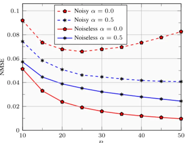
Fig. 1 shows the NMSE after convergence for different percentages of samples and parameter values. We observe that in the noiseless case the NMSE is reduced as the percentage increases. Moreover, the PG shows a larger error withα= 0.5 than with α = 0. This is because there are enough samples and β is small enough to allow the non-regularized PG to attain a low recovery error. In the noisy case, Fig. 1 shows that the error also decreases with Ps forα= 0.5, although it rises for α= 0 after Ps = 25%. This is due to the absence of regularization, which causes the PG to overfit to the noisy entries thus resulting in a larger error as more observations and noise are added.
Fig. 2 shows the evolution of the NMSE for Ps = 30% for the first 200 iterations for noisy and noiseless observations with different parameter values. We observe that the starting point of the PG with noiseless observations is fairly close to
10 20 30 40 50 0 0.02 0.04 0.06 0.08 0.1 Ps NMSE Noisyα= 0.0 Noisyα= 0.5 Noiselessα= 0.0 Noiselessα= 0.5
Figure 1: NMSE vs.Psfor noisy and noiseless observations.
0 50 100 150 200 0 0.02 0.04 0.06 0.08 0.1 0.12 Iteration NMSE Noisyα= 0.0 Noisyα= 0.5 Noiselessα= 0.0 Noiselessα= 0.5
Figure 2: NMSE vs. iterations withPs= 30%for noisy and noiseless observations.
the minimum since the initial estimate calculated with (4) has a very low NMSE equal to 0.033. For comparison, if we initialize to matrix M the NMSE is 0.699 and it takes 400 iterations to converge with α= 0. Forα= 0.5, the PG converges to a point close to the initial error. In the noisy case, we observe a smaller error at convergence forα= 0.5 than for α = 0, which converges to NMSE = 0.069 (see Fig. 1), since the graph regularization helps filter out some of the noise. Moreover, the regularization also increases the convergence speed with noisy observations since the PG with
α = 0 needs 1000 iterations to converge at Ps = 30%.
Regarding the convergence speed in all the scenarios, it should be noted that there exist implementations of the PG such as the one in [14] that accelerate the convergence.
From these simulations we can conclude that, if the random sampling is able to capture the underlying structure of the dataset and β is small enough, the Laplacian regularization does not reduce the recovery error when the observations are noiseless. On the other hand, with noisy observations the regularization improves the error for datasets which are smooth on the graph since it helps filter out the noise, prevents the overfitting to the observed noisy entries, and it also reduces the iterations to convergence. Finally, the proposed initialization provides a good starting point much closer to the minimum than the observed matrix.
REFERENCES
[1] E. J. Cand`es and B. Recht, “Exact matrix completion via convex optimization,”Foundations of Computational mathematics, vol. 9, no. 6, pp. 717–772, 2009.
[2] E. J. Candes and Y. Plan, “Matrix completion with noise,”Proceedings of the IEEE, vol. 98, no. 6, pp. 925–936, 2010.
[3] G. Liu and P. Li, “Advancing Matrix Completion by Modeling Extra Structures beyond Low-Rankness,” arXiv preprint arXiv:1404.4646, 2014.
[4] J. Cheng, Q. Ye, H. Jiang, D. Wang, and C. Wang, “STCDG: An efficient data gathering algorithm based on matrix completion for wireless sensor networks,” Wireless Communications, IEEE Transactions on, vol. 12, no. 2, pp. 850–861, 2013.
[5] A. Gogna and A. Majumdar, “Matrix completion incorporating auxiliary information for recommender system design,” Expert Systems with Applications, vol. 42, no. 14, pp. 5789–5799, 2015.
[6] D. I. Shuman, S. K. Narang, P. Frossard, A. Ortega, and P. Van-dergheynst, “The emerging field of signal processing on graphs: Ex-tending high-dimensional data analysis to networks and other irregular domains,”Signal Processing Magazine, IEEE, vol. 30, no. 3, pp. 83–98, 2013.
[7] A. Sandryhaila and J. M. Moura, “Discrete signal processing on graphs,”
IEEE transactions on signal processing, vol. 61, pp. 1644–1656, 2013. [8] T. Jebara, J. Wang, and S.-F. Chang, “Graph construction and b-matching for semi-supervised learning,” in Proceedings of the 26th Annual International Conference on Machine Learning. ACM, 2009, pp. 441–448.
[9] V. Kalofolias, X. Bresson, M. Bronstein, and P. Vandergheynst, “Matrix Completion on Graphs,”arXiv preprint arXiv:1408.1717, 2014. [10] S. Chen, A. Sandryhaila, J. M. Moura, and J. Kovaˇcevi´c, “Signal
Recovery on Graphs,”arXiv preprint arXiv:1411.7414, 2014. [11] N. Rao, H.-F. Yu, P. K. Ravikumar, and I. S. Dhillon, “Collaborative
filtering with graph information: Consistency and scalable methods,” in
Advances in Neural Information Processing Systems, 2015, pp. 2107– 2115.
[12] K. Hou, Z. Zhou, A. M.-C. So, and Z.-Q. Luo, “On the linear conver-gence of the proximal gradient method for trace norm regularization,” in
Advances in Neural Information Processing Systems, 2013, pp. 710–718. [13] K. Yi, J. Wan, T. Bao, and L. Yao, “A DCT regularized matrix completion algorithm for energy efficient data gathering in wireless sensor networks,”International Journal of Distributed Sensor Networks, vol. 2015, p. 96, 2015.
[14] S. Ma, D. Goldfarb, and L. Chen, “Fixed point and Bregman iterative methods for matrix rank minimization,”Mathematical Programming, vol. 128, no. 1-2, pp. 321–353, 2011.
[15] R. Sun, “Matrix completion via nonconvex factorization: Algorithms and theory,” Ph.D. dissertation, UNIVERSITY OF MINNESOTA, 2015. [16] A. Beck and M. Teboulle, “A fast iterative shrinkage-thresholding
algo-rithm for linear inverse problems,”SIAM Journal on Imaging Sciences, vol. 2, no. 1, pp. 183–202, 2009.