Handling continuous attributes in ant colony classification algorithms

Handling Continuous Attributes in Ant Colony

Classification Algorithms

Fernando E. B. Otero, Alex A. Freitas, and Colin G. Johnson

Abstract— Most real-world classification problems involve continuous (real-valued) attributes, as well as, nominal (dis-crete) attributes. The majority of Ant Colony Optimisation (ACO) classification algorithms have the limitation of only being able to cope with nominal attributes directly. Extending the approach for coping with continuous attributes presented by cAnt-Miner (Ant-Miner coping with continuous attributes), in this paper we propose two new methods for handling continuous attributes in ACO classification algorithms. The first method allows a more flexible representation of continuous attributes’ intervals. The second method explores the problem of attribute interaction, which originates from the way that continuous attributes are handled in cAnt-Miner, in order to implement an improved pheromone updating method. Empirical evaluation on eight publicly available data sets shows that the proposed methods facilitate the discovery of more accurate classification models.

I. INTRODUCTION

T

HE classification task in data mining aims at predicting the value of a given goal attribute for an example, based on the values of a set of predictor attributes for that example [1]. Since real-world classification problems are generally described by nominal (discrete) and continuous (real-valued) attributes, classification algorithms are required to be able to cope with both nominal and continuous attributes in order to build a classification model. However, most Ant Colony Optimisation (ACO) [2] classification algorithms have the limitation of being able to cope with only nominal attributes. Continuous attributes, if present, need to be transformed into nominal attributes, by creating discrete intervals in a preprocessing step. There are potentially two drawbacks by not coping with continuous attributes directly. Firstly, there is a need for a discretisation procedure in a preprocessing step. Secondly, less information is available to the classification algorithm, since the discretisation procedure creates a fixed number of discrete intervals for each continuous attribute.

In this paper, we focus on extending the ideas of c Ant-Miner [3] in coping with continuous attributes. cAnt-Miner pioneered in coping with both types (nominal and contin-uous) attributes directly, taking full advantage of all con-tinuous attributes’ information and not requiring a discreti-sation procedure in a preprocessing step. We propose two new methods for handling continuous attributes in ACO classification algorithms. The first method gives the ability to use continuous attributes intervals with lower and upper bound values (i.e.vlower≤attribute < vupper). The second

The authors are with the Computing Laboratory, University of Kent, Canterbury, Kent, United Kingdom (email: {febo2, A.A.Freitas, C.G.Johnson}@kent.ac.uk).

method explores the attribute interaction introduced by the way that continuous attributes are handled internally, which is not taken into account bycAnt-Miner. We present empirical evaluation results for validating the proposed methods.

The remainder of this paper is organised as follows. Section II presents a brief overview of Ant-Miner [4], the first ACO classification algorithm, and cAnt-Miner. Section III discusses the proposed two new methods for handling continuous attributes. The empirical evaluation results are presented in Section IV. Finally, Section V draws the con-clusions of the paper and present future research directions.

II. BACKGROUND

Ant Colony Optimisation (ACO) systems simulate the behaviour of real ants using a colony of artificial ants, which cooperate in finding good solutions to optimization problems. Each artificial ant, representing a simple agent in the system, builds candidate solutions to the problem at hand and communicates indirectly with other artificial ants by means of pheromone levels. At the same time that ants perform a global search for new solutions, the search is guided to better regions of the search space based on the quality of solutions found so far. The system converges to good solutions as a result of the collaborative interaction among the ants. The interactive process of building candidate solutions and updating pheromone values allows an ACO algorithm to converge to optimal or near-optimal solutions.

In the context of discovering classification rules in data mining, ACO algorithms have been successfully applied to several different classification problems [5]. In this section, we present an overview of Ant-Miner, the first implemen-tation of an ACO algorithm for the classification task of data mining [4], andcAnt-Miner [3], the first (to the best of our knowledge) ACO classification algorithm able to cope with continuous attributes without requiring a discretisation procedure in a preprocessing step.

A. Ant-Miner Overview

Ant-Miner aims at extractingIF-THENclassification rules of the formIF(term1)AND(term2)AND ... AND(termn) THEN (class) from data. Each term in the rule is a triple (attribute, operator, value), where operator represents a relational operator andvaluerepresents a value of the domain of attribute (e.g.sex=male). TheIF part corresponds to the rule’s antecedent and theTHEN part corresponds to the rule’s consequent, which represents the class to be predicted by the rule. An example that satisfies the rule’s antecedent

will be assigned the class predicted by the rule. As Ant-Miner only works with nominal (categorical or discrete) attributes, the only valid relational operator is “=” (equality operator). Continuous attributes need to be discretised in a preprocessing step.

A high level pseudo-code of Ant-Miner is presented in Algorithm 1 [4]. In summary, Ant-Miner works as follows. It starts with an empty rule list and iteratively (while loop) adds one rule at a time to that list while the number of uncovered training examples is greater than a user-specified maximum value. In order to construct rules, ants start with an empty rule (no terms in its antecedent) and add one term at a time to their rule antecedent (repeat-untilloop). Terms are probabilistically chosen to be added to current partial rules based on the values of the amount of pheromone (τ) and a problem-dependent heuristic information (η) associated with terms (vertices in the construction graph). A pheromone value and a heuristic value are associated with each possible term – i.e. each possible triple (attribute,operator,value). As usual in ACO, heuristic values are fixed (based on an information theoretical measure of the predictive power of the term), while pheromone values are iteratively updated based on the quality of the rules built by ants. Ants keep adding a term to their partial rule until any term added to their rule’s antecedent would make their rule cover less training examples than a user-specified threshold (in order to avoid too specific and unreliable rules), or all attributes have already been used. The latter rule construction stopping cri-terion is necessary because an attribute can only occur once in the antecedent of a rule, in order to avoid inconsistencies such as <sex = male AND sex = f emale>. Once the rule construction process has finished, the rule constructed by an ant is pruned to remove irrelevant terms from the rule antecedent. Then, the consequent of a rule is chosen to be the class value most frequent among the set of training examples covered by the rule in question. Finally, pheromone trails are updated using the best rule, based on a quality measureQ, created by ants. The process of constructing a rule is repeated until a user-specified number of iterations has been reached, or the best rule of the current iteration is exactly the same as the best rule constructed by a predefined number of previous iterations, which works as a rule convergence test. The best rule found along this iterative process is added to the rule list and the covered training examples (training examples that satisfy the antecedent of the best rule) are removed from the training set.

B. cAnt-Miner Overview

In order to overcome Ant-Miner’s limitation of only cop-ing with nominal attributes, Otero et al. [3] have proposed an Ant-Miner extension — named cAnt-Miner (Ant-Miner coping with continuous attributes) — which can dynamically create thresholds on continuous attributes’ domain values during the rule construction process. Since cAnt-Miner has the ability of coping with continuous attributes “on-the-fly”, continuous attributes do not need to be discretised in

Algorithm 1: High level pseudo-code of Ant-Miner. beginAnt-Miner

tr set←all training examples;

rule list← ∅;

while|tr set|> M axU ncoveredExamplesdo

τ←initializes pheromones; rulebest← ∅; repeat CreateRules(); ComputeConsequents(); P runeRules();

currentbest←BestRule();

U pdateP heromones(τ, currentbest); ifQ(currentbest)> Q(rulebest)then

rulebest←currentbest; end

i←i+ 1;

untili≥M axIterationsORConvergence();

rule list←rule list+rulebest;

tr set←tr set\CoveredExamples(rulebest); end

end

a preprocessing step. cAnt-Miner extended Ant-Miner in several ways, as follows.

Firstly,cAnt-Miner includes vertices to represent continu-ous attributes in the construction graph. For each nominal attribute xi and value vij (where xi is the i-th nominal attribute andvij is thej-th value belonging to the domain of

xi), a vertex (xi =vij) is added to the construction graph, as in Ant-Miner. Furthermore, for eachcontinuous attribute

yi, a vertex (yi) is added to the construction graph, unlike in Ant-Miner. Note that continuous attributes vertices do not represent a valid term, since they do not have a relational operator and value associated in the construction graph, in contrast to nominal attributes. The relational operator and a threshold value will be determined when an ant selects a continuous attribute vertex as the next term to be added to the rule (an example of continuous attribute term is: ‘age

>21’). This makes the choice of a relational operator and value tailored to the current candidate rule being constructed, rather than chosen in a static preprocessing step.

Secondly, in order to compute the heuristic information for continuous attributes,cAnt-Miner incorporates a dynamic entropy-based discretisation procedure. In Ant-Miner, the heuristic value of each nominal vertex (xi=vij) involves a measure of entropy associated with the partition of examples which have the specific vij value for the attribute xi. The entropy measure, which is derived from information theory and is often used in data mining, quantifies the impurity of a collection of examples. Since continuous attribute vertices (yi) do not represent a partition of examples as nominal attribute vertices, a threshold value v need to be selected in order to dynamically partition the set of examples into two intervals:yi < v andyi ≥v. The best threshold value

v is the value v that minimizes the entropy of the partition, computed as entropy(yi, v) = |Syi<v| |S| ·entropy(Syi<v) + |Syi≥v| |S| ·entropy(Syi≥v), (1)

where|Syi<v|is the total number of examples in the partition yi< v(partition of training examples where the attribute yi has a value less thanv),|Syi≥v| is the total number of

ex-amples in the partitionyi≥v(partition of training examples where the attribute yi has a value greater or equal tov) and |S|is the total number of training examples. The values of

entropy(Syi<v)andentropy(Syi≥v)are computed as

entropy(T) =

k X c=1

−p(c|T)·log2p(c|T), (2) wherep(c|T)is the proportion of examples inT that have classcandkis the number of classes. After selection of the best threshold value v using Equation (1), the measure of entropy used to calculate the heuristic value of the continuous attribute vertex (yi) corresponds to the minimum entropy value between the two generated intervals (yi < v) and (yi≥v), according to Equation (2).

Thirdly, when a continuous attribute vertex (yi) is selected by an ant to be added to its current partial rule, a relational operator and a value is computed using a similar procedure as for the heuristic information. The best threshold value

v is selected using Equation (1), subject to the restriction of considering only examples covered by the current partial rule in the evaluation of threshold values. Then, the relational operator (‘<’ or ‘≥’) associated with the interval with the lowest entropy value is selected and a term in the form (yi, operator,v) added to the ant’s current partial rule (e.g. age

<18).

Fourthly, the pheromone updating procedure has been extended to cope with continuous attribute vertices. In the case of continuous attributes, pheromone values are associ-ated with continuous attribute vertices not considering the operator and threshold value, that is, there is a single entry in the pheromone matrix for each continuous attribute, in contrast to multiple entry for nominal attributes — nominal attributes have an entry for every (xi,vij) pair.

III. NEWMETHODS FORHANDLINGCONTINUOUS

ATTRIBUTES INANTCOLONYCLASSIFICATION

ALGORITHMS

Extending on the ideas ofcAnt-Miner, this paper presents two new methods for handling continuous attributes in Ant Colony Optimisation (ACO) classification algorithms. The first method enables the creation of intervals with both lower and upper bound values for continuous attributes, in the form of vlower ≤ attribute < vupper, by incorporating a new dynamic discretisation procedure based on the Minimum

Description Length (MDL) principle [6] in the rule construc-tion process. The second method explores the fact that the discretisation of continuous attributes occurs when an ant selects a continuous attribute vertex to be added to its current partial rule. Since only examples covered by the current partial rule are considered for the threshold calculation, the previously selected vertices play an important role in the creation of discrete intervals. The order dependency between vertices in a rule characterizes an attribute interaction, which is not taken into account by cAnt-Miner.

A. MDL-based Discretisation

Fayyad and Irani [6] presented an MDL-based approach where multiple discrete intervals can be extracted by apply-ing a binary discretisation procedure recursively, selectapply-ing the best threshold value at each iteration, and using the minimal description length principle as a stopping criterion to deter-mine whether more threshold values should be introduced. The motivation for multiple interval discretisation lay in the fact that the ‘interesting’ value range may be an internal interval (e.g. 18 ≤ age < 21), which can not be easily generated by a binary-interval-at-a-time discretisation pro-cedure. The MDL-based approach generally leads to coarse intervals in cases where the examples are homogeneously distributed (distributed in a few different class values) and to fine intervals in cases of more uniform distributions.

Following Fayyad and Irani, we have incorporated a MDL-based decision criterion to decide whether or not to split a given interval further in cAnt-Miner. The basic idea is to apply cAnt-Miner’s entropy-based discretisation method recursively, relying on the MDL criterion to accept or reject a threshold value. In this way, instead of generating only intervals in the form yi < v and yi ≥ v, internal intervals in the form vlower ≤yi < vupper can be created (where v,

vlower andvupper are values in the domain of the continuous attributeyi).

The MDL-based discretisation method is divided in two steps, as follows. In the first step, the best threshold value

v for a continuous attribute vertex (yi) is selected as in the originalcAnt-Miner — Equation (1). In the second step, the MDL decision criterion for accepting or rejecting a threshold value v is computed as Gain(yi, v;S)> log2(|S| −1) |S| + ∆(yi, v;S) |S| , (3) Gain(yi, v;S) =entropy(S) −|Syi<v| |S| ·entropy(Syi<v) −|Syi≥v| |S| ·entropy(Syi≥v), (4) ∆(yi, v;S) =log2(3k−2)−[k·entropy(S) −kyi<v·entropy(Syi<v)

−kyi≥v·entropy(Syi≥v)], (5)

wherek,kyi<v andkyi≥v are the number of different class

values in S, Syi<v and Syi≥v, respectively. If the MDL

criterion defined in Equation (3) is satisfied, the threshold valuevfor the continuous attributeyiis accepted; otherwise it is rejected. Note that the entropy measures of S, Syi<v

andSyi≥v required to evaluate the threshold valuev against the MDL criterion are already computed by the first step (threshold selection). Therefore, there is no increase in com-putational time to compute the MDL criterion. Finally, if the threshold valuev is accepted, the discretisation procedure is repeated individually for the partitionsSyi<v andSyi≥v.

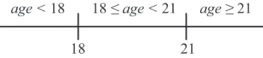
At the end of the MDL discretisation procedure, we can have potentially multiple threshold values. In order to select the best threshold value(s), the list of threshold values is sorted and the entropy value for each discrete interval is calculated. Then, the interval with the lowest entropy value is selected (based on the fact that lower entropy values represent more “pure” partitions where most of the examples belong to a single class). If an internal interval is selected (an interval between two threshold values), a term in the form vj ≤yi< vj+1 is generated; otherwise, a term in the form yi < vj or yi ≥ vj is generated (where j is the j-th threshold value selected). Fig. 1 illustrates the intervals that could have been created by selecting two threshold values for a continuous attributeage.

18 _{≤ age <} 21 _{age ≥} 21 age < 18

18 21

Fig. 1. Illustration of discrete intervals that that could have been created by selecting two threshold values for a continuous attributeage. At the end of the MDL discretisation procedure, the interval associated with the lowest entropy value is selected.

B. Encoding Attribute Interaction as Pheromone Levels: Associating Pheromones with Edges

In the original version of Ant-Miner, pheromone values are associated with vertices in the construction graph, where each vertex represents a term xi =vij (e.g.sex= male). Hence, both ants with rule antecedents<sex=maleAND

smoke=no>and<smoke=noANDsex=male>will deposit the same amount of pheromone on vertices ‘sex= male’ and ‘smoke=no’.

cAnt-Miner employs the same pheromone update proce-dure, even though the order of attributes (vertices) could affect the threshold values of continuous attributes. Note that this attribute interaction dependency is not observed in the original Ant-Miner, since it only supports nominal attribute vertices which are represented by <attribute = value>

pairs and their order is irrelevant. For instance, a partial rule with a term <sex = male> followed by a term

<smoke = no> has no difference is comparison with a partial rule with a term<smoke=no>followed by a term

<sex = male>. On the other hand, a partial rule with a

term <smoke= no>followed by a term representing the continuous attribute age is different in comparison with a partial rule with a term representing a continuous attribute age followed by a term <smoke=no>. In the first case, only examples covered by the partial rule<smoke =no>

are used to compute a threshold value for the continuous attributeage (e.g.age <10). In the latter case, all examples of the training set are used to compute a threshold value for the continuous attribute age (e.g. age ≥ 25) since the continuous attributeageis the first attribute to be added to the rule. Although the discretisation procedure is deterministic, there is no guarantee that the same values will be chosen since the examples used to compute the threshold values are different. This might affect the way that ants explore the construction graph, since the pheromone levels do not accurately reflect paths explored by previous ants.

A straightforward implementation to preserve the order is to associate pheromone on the edges instead of vertices. For instance, when updating pheromones levels for a rule

<smoke = no AND age < 10>, instead of depositing the pheromone on the vertices ‘sex = male’ and ‘age’, the pheromone is deposited on the edge that connects the vertex ‘sex = male’ to the vertex ‘age’. Consequently, when updating pheromone levels for a rule<age≥25AND

smoke = no>, the pheromone is deposited on the edge that connects the vertex ‘age’ to the vertex ‘smoke=no’. Note that even though the construction graph is conceptually defined as a fully connected (bidirectional edges) graph, in practice there is one edge for each direction between each pair of vertices. To be able to associate pheromone levels to the first vertex of a rule, a dummy vertex ‘start’ is added and unidirectionally connected to all vertices in the construction graph. This vertex represents the starting point for creating trails and its purpose is to associate pheromone values on the edge of the first attribute vertex of an ant’s trail.

In order to calculate the probability of selecting a vertex to be added to the current partial rule, the pheromone value associated with the edge between the last vertex of the rule (or the dummy ‘start’ vertex when the rule is empty) and the candidate vertex is used in combination with the heuristic value associated with the candidate vertex in the same manner as in Ant-Miner and cAnt-Miner. The main advantage of this method can be seen when dealing with continuous attributes. Since the dynamic discretisation pro-cedure of continuous attributes is deterministic and based on the current covered examples, as discussed previously, using pheromone levels to represent the order in which ants select vertices to compose candidate rules indirectly preserves the threshold values of continuous attributes.

The idea of associating pheromone values with the edges of the construction graph have been previously explored in AntMiner+ by Martens et al. [7], although it was used in a very different context. The construction graph in AntMiner+ is defined as a direct acyclic graph (DAG). Therefore, the attribute order is explicitly determined by the construction graph DAG-structure, rather than by pheromone levels on

the edges between vertices as proposed in this work, which has the undesirable bias of restricting ants to create trails following a specific order of attributes.

As discussed in subsection II-A, after an ant completes the rule’s construction process, the created rule undergoes a pruning procedure which aims at removing irrelevant terms that might have been included in the rule. The original pruning procedure employed by Ant-Miner and cAnt-Miner consists of removing one term at a time while this procedure improves the quality of the rule. Therefore, at each iteration of the pruning procedure,n(wherenis the number of terms in the current rule) candidate rules with n−1 terms are evaluated and the rule with highest quality is selected for further pruning. This procedure is repeated until no term can be removed which improves the current rule quality or the current rule has only one term left. Clearly, the original pruning procedure does not take into account the order in which terms appear in a rule. For instance, a rule

<sex = male AND age ≥ 25 AND smoke= yes>can be pruned to <age≥25AND smoke=yes>, which will update the pheromone levels considering ‘age’ as the first vertex of the rule followed by the vertex ‘smoke = yes’. This is not consistent with how the threshold of the attribute

agewas calculated and there is no guarantee that, if an ant selects the vertex ‘age’ as the first term of its rule, it will have the same threshold value (‘25’ in this case).

To avoid such inconsistencies, we proposed a new pruning procedure (dubbed ‘threshold-aware’ pruning) sensible to the order of attributes (vertices). Since the order of terms in a rule is consistent with continuous attributes threshold values, a simple implementation of a threshold-aware pruning is to remove the last term that was added to the rule in order to simplify the rule. The removal process is repeated until the rule quality decreases when the last term is removed or the rule has only one term left. Note that, in this procedure, the continuous attribute threshold values do not have to be re-calculated, since terms are removed in the reverse order that they were added to the rule. Also, only one candidate rule has to be evaluated at each iteration of the pruning procedure, resulting in a more efficient pruning procedure when compared to the original one employed by Ant-Miner andcAnt-Miner.

IV. COMPUTATIONALRESULTS

The proposed cAnt-Miner extensions were evaluated us-ing eight publicly available data sets from the UCI Irvine machine learning repository [8]. We selected data sets that contain at least one continuous attribute, since our goal is to evaluate the different proposed variations of cAnt-Miner, using the original Ant-Miner as a baseline method. We also include the results for J48 (Weka [9] implementation of the well-known C4.5 decision tree algorithm [10]) using the same data sets. We evaluated the proposed cAnt-Miner extensions individually, and also the combination of both, generating three variations of cAnt-Miner. Table I summa-rizes the different classifiers used in our experiments.

TABLE I

SUMMARY OF THE CLASSIFIER METHODS USED IN OUR EXPERIMENTS.

Classifier Description

Ant-Miner original Ant-Miner version

cAnt-Miner originalcAnt-Miner version cAnt-Miner-MDL MDL-basedcAnt-Miner

cAnt-Miner2 cAnt-Miner using pheromones on the edges cAnt-Miner2-MDL MDL-basedcAnt-Miner2

J48 Weka’s C4.5 implementation

TABLE II

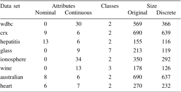
SUMMARY OF THE DATA SETS USED IN OUR EXPERIMENTS.

Data set Attributes Classes Size

Nominal Continuous Original Discrete

wdbc 0 30 2 569 366 crx 9 6 2 690 639 hepatitis 13 6 2 155 116 glass 0 9 7 213 119 ionosphere 0 34 2 350 292 wine 0 13 3 178 126 australian 8 6 2 690 637 heart 6 7 2 270 232

The experiments were conducted using a 10-fold cross-validation procedure [9]. For stochastic classifiers, i.e. Ant-Miner and cAnt-Miner variations, we run the classifier 10 times — using a different random seed to initialise the search each time — for each cross-validation fold. In the case of the deterministic J48 classifier, it is run just once for each cross-validation fold. Since the original version of Ant-Miner does not cope with continuous attributes directly, the data sets were discretised in a preprocessing step. For each cross-validation fold, we separately discretised (using the C4.5-Disc discretisation method [11]) the training set and the created discrete intervals were used to discretise the test set. This separation is necessary because, if we had discretised the entire dataset before creating the cross-validation folds, the discretisation method would had access to the test data. This would have compromised the reliability of the experi-ments. Moreover, we also removed the duplicated examples (examples with the same values for all attributes) from the resulting discrete dataset to avoid the possibility that a test set contains an example that is the same as a training example. Table II presents the summary of the data sets used in our experiments. In Table II, the first column gives the data set name, the second and third columns give the number of nominal and continuous attributes respectively, the fourth column gives the number of classes, the fifth column gives the number of examples in the original data set and the sixth column gives the number of examples in the discrete data set (after the removal of duplicated examples). Recall that only the original Ant-Miner used the discrete data sets.

TABLE III

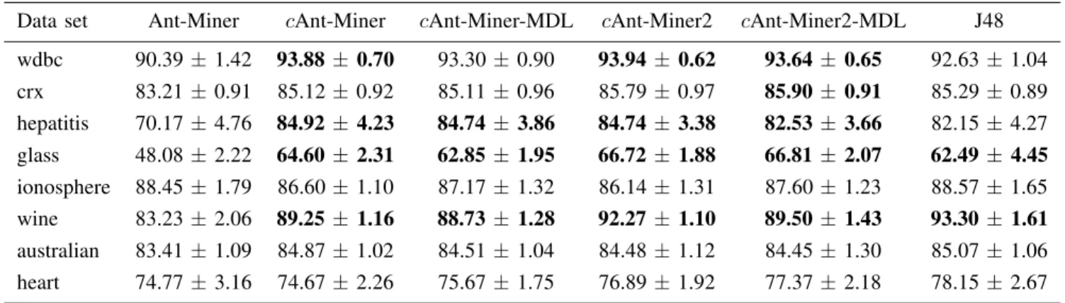
PREDICTIVE ACCURACY(mean±standard deviation)AFTER THE10-FOLD CROSS-VALIDATION PROCEDURE.

Data set Ant-Miner cAnt-Miner cAnt-Miner-MDL cAnt-Miner2 cAnt-Miner2-MDL J48 wdbc 90.39±1.42 93.88 ±0.70 93.30±0.90 93.94± 0.62 93.64 ±0.65 92.63±1.04 crx 83.21±0.91 85.12±0.92 85.11±0.96 85.79±0.97 85.90 ±0.91 85.29±0.89 hepatitis 70.17±4.76 84.92 ±4.23 84.74±3.86 84.74± 3.38 82.53 ±3.66 82.15±4.27 glass 48.08±2.22 64.60 ±2.31 62.85±1.95 66.72± 1.88 66.81 ±2.07 62.49±4.45 ionosphere 88.45±1.79 86.60±1.10 87.17±1.32 86.14±1.31 87.60±1.23 88.57±1.65 wine 83.23±2.06 89.25 ±1.16 88.73±1.28 92.27± 1.10 89.50 ±1.43 93.30±1.61 australian 83.41±1.09 84.87±1.02 84.51±1.04 84.48±1.12 84.45±1.30 85.07±1.06 heart 74.77±3.16 74.67±2.26 75.67±1.75 76.89±1.92 77.37±2.18 78.15±2.67

classifier on the data sets used in our experiments. Each entry in the table corresponds to the average value of accu-racy obtained using the 10-fold cross-validation procedure, followed by the standard deviation. In addition, an entry is shown in bold if, for the corresponding data set, the accuracy obtained by the corresponding classifier was significantly greater than the accuracy achieved by Ant-Miner for that data set — according to a two-tailed Student’s t-test with 95% confidence.

The results on Table III show that all variations of c Miner are able to obtain significant improvements over Ant-Miner (the baseline classifier in our experiments) in at least three out of eight data sets, namely hepatitis, glass and wine. The use of the MDL-based discretisation isolated was not effective in the wdbc data set, where cAnt-Miner-MDL obtained a higher accuracy value that was not statistically significant over Ant-Miner. The remaining three variations ofcMiner obtained significant improvements over Ant-Miner in the wdbc data set. Furthermore, the combination of both proposed extensions enabled cAnt-Miner2-MDL to obtain significant improvements over Ant-Miner in the crx data set. On the other hand, J48 significantly outperformed Ant-Miner only in two data sets, namely glass and wine.

The results obtained in the experiments can be summa-rizes as follows. Overall, cAnt-Miner2-MDL is the most accurate classifier method compared to the baseline Ant-Miner classifier. In five of eight data sets, c Ant-Miner2-MDL significantly outperformed Ant-Miner. In the remaining three data sets, there were no significant differences between

cAnt-Miner2-MDL and Ant-Miner. Although there are no significant differences between cAnt-Miner variations and J48, it should be noted that J48 was able to significantly outperform the baseline Ant-Miner only in two out of eight data sets.

V. CONCLUSIONS

In this paper, we have presented two new methods con-cerning the handling of continuous attributes in ACO classi-fication algorithms. Following the ideas ofcAnt-Miner (Ant-Miner coping with continuous attributes), a new

discretisa-tion procedure based on the MDL principle was incorporated in the rule construction process, allowing the creation of discrete intervals using lower and upper bound values (i.e.

vlower ≤attribute < vupper). Furthermore, it was proposed to deposit the pheromone on edges instead of vertices of the construction graph in order to deal with attribute interaction introduced by the way that the rule construction process copes with continuous attributes in cAnt-Miner.

We have performed experiments comparing the perfor-mance of Ant-Miner,cAnt-Miner, three variations ofc Ant-Miner which incorporate the proposed methods, and J48 (Weka’s C4.5 implementation). Using Ant-Miner as a base-line classifier, all cAnt-Miner variations (including the orig-inalcAnt-Miner) significantly outperformed Ant-Miner in at least three out of eight data sets. The incorporation of both proposed methods into cAnt-Miner, dubbed c Ant-Miner2-MDL, significantly outperformed Ant-Miner in five out of eight data sets. There were no significant differences between

cAnt-Miner variations and J48. On the other hand, J48 significantly outperformed Ant-Miner only in two data sets. As future research direction, it would be interesting to investigate the performance of different discretisation meth-ods in the rule construction process. Also, since depositing pheromone on the edges leads to a modified pruning proce-dure, evaluating other kinds of pheromone updating strategies is also a direction worth further exploration.

ACKNOWLEDGEMENTS

The authors acknowledge the financial support from an Eu-ropean Union’s INTERREG project (Ref. No. 162/025/361). Fernando Otero also acknowledges further financial support from the Computing Laboratory, University of Kent.

REFERENCES

[1] U. Fayyad, G. Piatetsky-Shapiro, and P. Smith, “From data mining to knowledge discovery: an overview,” in Advances in Knowledge Discovery & Data Mining, U. Fayyad, G. Piatetsky-Shapiro, P. Smith, and R. Uthurusamy, Eds. MIT Press, 1996, pp. 1–34.

[2] M. Dorigo and T. St¨utzle,Ant Colony Optimization. MIT Press, 2004. [3] F. Otero, A. Freitas, and C.G.Johnson, “cAnt-Miner: an ant colony classification algorithm to cope with continuous attributes,” inAnt Colony Optimization and Swarm Intelligence (Proc. ANTS 2008), LNCS 5217. Springer, 2008, pp. 48–59.

[4] R. Parpinelli, H. Lopes, and A. Freitas, “Data mining with an ant colony optimization algorithm,”IEEE Transactions on Evolutionary Computation, vol. 6, no. 4, pp. 321–332, 2002.

[5] A. Freitas, R. Parpinelli, and H. Lopes, “Ant colony algorithms for data classification,” To apper inEncyclopedia of Info. Sci. & Tech. 2nd Ed, 2008.

[6] U. Fayyad and K. Irani, “Multi-interval discretization of continuous-valued attributes for classification learning,” inThirteenth International Joint Conference on Artifical Inteligence. Morgan Kaufmann, 1993, pp. 1022–1027.

[7] D. Martens, M. D. Backer, R. Haesen, J. Vanthienen, M. Snoeck, and B. Baesens, “Classification with ant colony optimization,”IEEE Transactions on Evolutionary Computation, vol. 11, no. 5, pp. 651– 665, 2007.

[8] A. Asuncion and D. Newman, “UCI Machine Learning Repository,” http://www.ics.uci.edu/∼mlearn/MLRepository.html, 2007.

[9] H. Witten and E. Frank,Data Mining: Practical Machine Learning Tools and Techniques, 2nd ed. Morgan Kaufmann, 2005.

[10] J. Quinlan, C4.5: Programs for Machine Learning. Morgan Kauf-mann, 1993.

[11] R. Kohavi and M. Sahami, “Error-based and entropy-based discretiza-tion of continuous features,” inProceedings of the 2nd International Conference Knowledge Discovery and Data Mining. AAAI Press, 1996, pp. 114–119.