Rowan University Rowan University
Rowan Digital Works
Rowan Digital Works
Theses and Dissertations 12-12-2012
Hybrid solvers for the Boolean Satisfiability problem: an
Hybrid solvers for the Boolean Satisfiability problem: an
exploration
exploration
Nicole NelsonFollow this and additional works at: https://rdw.rowan.edu/etd
Part of the Computer Sciences Commons
Let us know how access to this document benefits you -
share your thoughts on our feedback form.
Recommended Citation Recommended Citation
Nelson, Nicole, "Hybrid solvers for the Boolean Satisfiability problem: an exploration" (2012). Theses and Dissertations. 239.
https://rdw.rowan.edu/etd/239
This Thesis is brought to you for free and open access by Rowan Digital Works. It has been accepted for inclusion in Theses and Dissertations by an authorized administrator of Rowan Digital Works. For more information, please contact [email protected].
HYBRID SOLVERS FOR THE BOOLEAN SATISFIABILITY PROBLEM: AN EXPLORATION
by
Nicole Ann Nelson
A Masters Thesis Submitted to the
Department of Computer Science College of Liberal Arts and Sciences In partial fulfillment of the requirement
For the degree of Masters of Science
at
Rowan University December 5th, 2012 Thesis Chair: Dr. Andrea F. Lobo
Acknowledgements
First of all, I would like to acknowledge my parents for their continued support through my educational career. From a very young age I learned to work hard to achieve, and as the tasks became more challenging I have worked even harder. Thanks to my parents’ encouragement to do well and excel, I am the successful student and professional I am today.
Second, I would like to acknowledge my siblings and boyfriend for their support throughout my studies. The understanding and acceptance for the months that I had no time for anything but thesis was invaluable in my success. I am especially thankful for the more challenging days when they were able to make me laugh, even if it only lifted the weight off my shoulders momentarily.
I would also like to thank Dr. Andrea F. Lobo, Dr. Ganesh R. Baliga, and Dr. Vasil Hnatyshin for their time and contributions as a part of my thesis committee. I would especially like to thank Dr. Baliga for his large contribution in the research conducted during my graduate studies. Without his guidance I wouldn’t be where I am today.
Abstract Nicole Ann Nelson
HYBRID SOLVERS FOR THE BOOLEAN SATISFIABILITY PROBLEM: AN EXPLORATION
Dr. Andrea F. Lobo
Masters of Science in Computer Science
The Boolean Satisfiability problem (SAT) is one of the most extensively researched NP-complete problems in Computer Science. This thesis focuses on the design of feasible solvers for this problem. A SAT problem instance is a formula in propositional logic. A SAT solver attempts to find a solution for the formula. Our research focuses on a newer solver paradigm, hybrid solvers, where two solvers are combined in order to gain the benefits from both solvers in the search for a solution. Our hybrid solver, AmbSAT, combines two well-known solvers: the systematic Davis-Putnam-Logemann-Loveland solver (DPLL) and the stochastic WalkSAT solver. AmbSAT’s design is original and differs from the hybrid solver designs in the research literature. AmbSAT utilizes a DPLL algorithm to lead the search and WalkSAT at appropriate points to aid in the search process. Central to AmbSAT’s design is the notion of ambivalence. Essentially, ambivalence attempts to formally identify the points in time when the DPLL solver might be well served by further guidance from WalkSAT. In this thesis, we present three different ambivalence notions and analyze their performance against a pure DPLL solver. Our results are promising, and indicate that AmbSAT performs better than a pure DPLL solver on a diverse collection of SAT problem instances.
Table of Contents
Abstract iv
Table of Figures vi
Chapter 1 Introduction 1
Chapter 2 SAT Solvers: A Survey 4
2.1 Terminology 4
2.2 Complete Solvers 6
2.3 Incomplete Solvers 13
2.4 Hybrid Solvers 16
Chapter 3 AmbSAT: A Complete Hybrid Solver 20
3.1 Basic Concepts 20
3.2 Designing for Efficiency 21
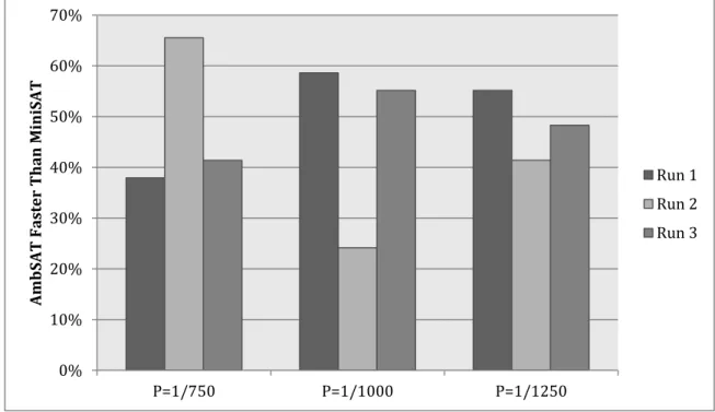
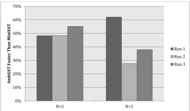
3.3 Experimentation Methodology 25 3.4 Design Settings 27 3.5 Implementation Details 31 3.6 Ambivalence Notions 36 3.6.1 Probabilistic Ambivalence. 37 3.6.2 Equality Ambivalence. 38
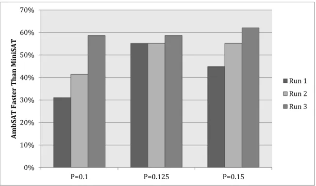
3.6.3 Normalized Percentage Ambivalence. 40
3.7 Conclusions and Future Work 42
List of References 46
Appendix A Benchmark Problem Set Details 49
Appendix B Details of MiniSAT’s Performance on the Benchmark Problem Set 50 Appendix C Details of AmbSAT’s Performance with 5% Scout Overhead on the
Benchmark Problem Set 51
Appendix D Details of AmbSAT’s Performance with Polarity Selection Strategy on the
Benchmark Problem Set 52
Appendix E AmbSAT’s Modified Heap Implementation Details 53
Appendix F Ambivalence Notion Implementation Details 54
Appendix G Details of AmbSAT’s with Probability Ambivalence Performance with
P=1/1000 on the Benchmark Problem Set 57
Appendix H Details of AmbSAT’s with Equality Ambivalence Performance with N=2 on
the Benchmark Problem Set 58
Appendix I Details of AmbSAT’s with Normalized Percentage Ambivalence Performance
Table of Figures
Figure 1 DPLL Algorithm Pseudo Code ... 6
Figure 2 SLS Algorithm Pseudo Code ... 13
Figure 3 Shifting Assigned Variables ... 24
Figure 4 Performance of AmbSAT with Different Allowable Overhead Percentages vs. MiniSAT ... 28
Figure 5 Performance of AmbSAT Selection Strategies vs. MiniSAT ... 30
Figure 6 AmbSAT select Method: Pseudo Code ... 33
Figure 7 Performance of AmbSAT with Probabilistic Ambivalence vs. MiniSAT ... 38
Figure 8 Performance of AmbSAT with Equality Ambivalence vs. MiniSAT ... 40
Figure 9 Performance of AmbSAT with Normalized Percentage Ambivalence vs. MiniSAT ... 41
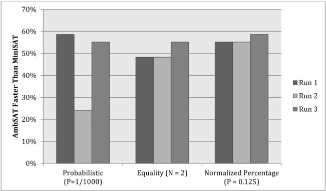
Figure 10 Performance of AmbSAT with Optimized Ambivalence Notions vs. MiniSAT ... 43
Figure 11 Sub-problem Clause Setup Implementation Details ... 53
Figure 12 Sub-problem Clause Maintenance Implementation Details ... 53
Figure 13 Ambivalence Abstract Class Implementation Details ... 54
Figure 14 Probabilistic Ambivalence Notion Implementation Details ... 54
Figure 15 N Equal Ambivalence Notion Implementation Details ... 55
Chapter 1 Introduction
The boolean satisfiability problem (SAT) is the problem of determining if a satisfying assignment exists for a given boolean constraint formula represented in conjunctive normal form (CNF). A solution is a boolean assignment that results in a true evaluation of the formula.
The SAT problem was proven by Stephen Cook to be the first NP-complete in 1971 [4]. The following year, Richard Karp used Cook’s results to prove 21 other problems to be NP-complete such as the Hamiltonian circuit problem, the 0-1 Knapsack problem, and the Clique problem [16]. NP-complete problems can be found in many diverse fields of research within and outside of Computer Science [8]. Any NP-complete problem can be translated using a translation that operates in polynomial time to any other NP-complete problem. So, a polynomial time solution to any NP-complete problem leads to a polynomial time solution to all problems in this collection. Such a solution would answer in the positive the most outstanding unanswered question in Computer Science, whether P = NP.1
The growing interest in the SAT problem correlates to the increasing number of applications of SAT. Applications of SAT include, but are not limited to: circuit verification, motion planning, scheduling, computer network design and automated reasoning. The biannual SAT competition is a result of this increased interest in the field of research. 2 Contestants in this competition can submit their SAT solvers as well as hard SAT problem instances. SAT problem instances at the SAT competition fall into three
1 http://www.claymath.org/millennium/
categories: application, crafted, and random. Application, also known as industrial, instances represent encodings of problems in which SAT might be useful for such as model checking and planning. Crafted instances represent the problem set designed to challenge SAT solvers; problems in which typical solvers have a hard time. Random instances represent problem sets produced by a generator based on a random seed.
There are many approaches for solving SAT problem instances. Broadly speaking, SAT solvers can be either complete or incomplete. A complete solver can conclusively make the decision whether a satisfying assignment exists for the formula in question. An incomplete solver can often find a satisfying assignment, if one exists, but cannot show that no assignment exists.
SAT solvers often fall into one of two paradigms: stochastic local search (SLS), and Davis-Putnam-Logemann-Loveland (DPLL). SLS solvers are incomplete SAT solvers. SLS solvers combine a randomized walk through the exponential sized search space of possible assignments with techniques from artificial intelligence such as hill climbing and simulated annealing. SLS solvers often operate with low memory requirements and excel on SAT instances from the random category. The DPLL algorithm is one of the most popular complete algorithms for solving SAT. DPLL is the basis for many high grade SAT solvers [6], [21], many of which have excelled at the recent SAT competitions. DPLL searches the assignment search space using backtracking. High grade DPLL implementations augment the basic algorithm with sophisticated techniques such as clause learning and fast constraint propagation using watched literals, which provide significant improvements in solver performance. They have a higher memory requirement than SLS solver and are considered the best solvers
for application and crafted problem instances. DPLL solvers typically perform poorly on random problem instances.
In recent years, a new breed of solvers called hybrid solvers have emerged. Hybrid solvers combine complete and incomplete solvers, and may themselves be complete or incomplete [2].The concept of hybrid solvers is to use two different solvers that excel in different areas of SAT formulas and combine them together to gain the benefits of both solvers. Typically, hybrid solvers are crafted using one of the following techniques:
1. Use an SLS solver to support a DPLL solver [5], [10]. 2. Use a DPLL solver to support an SLS solver [2], [9], [15].
3. Using the SLS and DPLL solver to equally aid one another [1], [7], [17], [19].
The research discussed in future chapters falls in the category of hybrid solvers. Our approach aims at utilizing a stochastic solver to aid the decision making process of a DPLL solver. Over time various techniques in this area have been developed. The goal of the research conducted is to determine a technique for combining two solvers into one that shows promise for competitive results.
The next chapter features a formal introduction to SAT and a detailed discussion of the DPLL and WalkSAT SLS solver. Chapter 3 features our abstract notion of
ambivalence which lies at the heart of our hybrid SAT solver. Additionally it focuses on the important design issues that have a bearing on the hybrid solver’s performance. Chapter 3 also discusses specific ambivalence notions and the results pertaining to each implementation. Lastly, conclusions are made based on the data presented.
Chapter 2 SAT Solvers: A Survey
This chapter includes in detail the most prominent approaches adopted by modern SAT solvers.
2.1 Terminology
A SAT formula is composed of boolean variables and the boolean operators or
(denoted ∨), and (denoted ∧), and negation (denoted -). The smallest building block in a SAT formula is a boolean variable which can take either a true or false value. A literal is a boolean variable represented in its positive or negative form. So, 4 and -4 are the literals corresponding to the boolean variable 4. A satisfying assignment for a literal is a truth value which evaluates the literal to true. For instance, the literal 4 is satisfied by the assignment true, and the literal -4 by the assignment false. A clause comprises of literals joined together by the boolean or operation. For example, (1 ∨ -2 ∨ -3 ∨ 4) is a clause comprising 4 literals. In order to satisfy a clause, at least one literal must evaluate to true. A satisfying assignment for a clause is an assignment that makes the clause true. For clause (1 ∨ -2 ∨ -3 ∨ 4), a satisfying assignment would be 1=false, 2=false, 3=true, 4=true. A SAT formula in conjunctive normal form (CNF) is a collection of clauses joined together by the boolean and operation. This thesis focuses exclusively on CNF formulae. In order for a formula to evaluate to true, each clause must evaluate to true. An assignment that satisfies each clause of a formula is said to satisfy the formula and is called a satisfying assignment for the formula. Formula 1 is satisfied by the assignment 1=false, 2=true, 3=false, and 4=false. Observe that the first clause is satisfied by 4=false,
the second clause is satisfied by either 2=true or 4=false, and the third clause is satisfied by 1=false. Note that the assignment 1=true, 2=true, 3=true, and 4=true is another satisfying assignment for this formula.
∨ ∨ ∧ ∨ ∧ ∨ (1)
A satisfying assignment may be either a complete or partial assignment of the variables represented in the formula. A partial assignment leaves some of the variables in the formula unassigned. For instance, Formula 1 can be satisfied by the partial assignment 2=true and 3=true, where variable 3 satisfies the first and third clause and variable 2 satisfies the second clause. A formula that has a satisfying assignment is called
satisfiable.
∨ ∨ ∧ ∨ ∧ ∨ ∧ ∨ ∧ ∨ ∨ (2)
For some formulas a satisfying assignment does not exist, these formulas are called unsatisfiable. Clearly, there are 2N possible assignments for a formula that has N
variables. Formula 2 is an unsatisfiable formula with three variables. In the case of Formula 2, none of the eight possible assignments to the three variables in the formula satisfies the formula.
The task of SAT solvers is to find a satisfying assignment for a formula, if one exists. SAT solvers are either incomplete or complete. Incomplete solvers can often find a
solution if one exists, but are unable to determine unsatisfiability. A complete solver can definitely determine a solution if one exists or declare unsatisfiability if no solution exists.
2.2 Complete Solvers
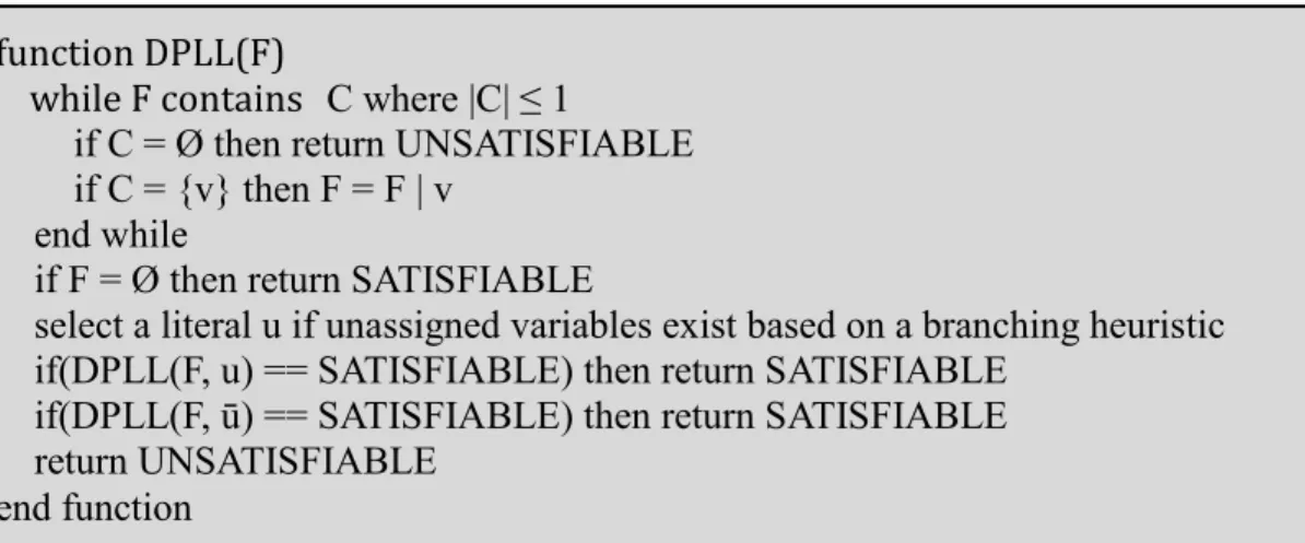
Complete solvers declare a formula as unsatisfiable when no satisfying assignment exists as well as find a satisfying assignment when one exists. The best performing complete SAT solvers are based on the Davis-Putnam-Logemann-Loveland (DPLL) algorithm. The set of all possible assignments to variables in a formula can be viewed as a binary tree. Leaves in the binary tree represent complete assignments or partial assignments that have been declared a dead-end. The internal nodes in this tree are partial assignments and the root node denotes the empty assignment. Each edge in the tree represents the assignment of a boolean variable in the formula to a true or false value. The DPLL algorithm uses backtracking to traverse this binary tree of assignments.
function DPLL(F)
while F contains C where |C| ≤ 1
if C = Ø then return UNSATISFIABLE if C = {v} then F = F | v
end while
if F = Ø then return SATISFIABLE
select a literal u if unassigned variables exist based on a branching heuristic if(DPLL(F, u) == SATISFIABLE) then return SATISFIABLE
if(DPLL(F, ū) == SATISFIABLE) then return SATISFIABLE return UNSATISFIABLE
end function
Figure 1 displays the pseudo code for a recursive implementation of the DPLL algorithm where F represents the formula, C represents the current clause, v represents the unit variable, u represents the variable selected by the branching heuristic, and ū represents the negation of variable u. The algorithm traverses the tree by assigning unassigned variables to true or false values. The partial assignment at a node in the tree will satisfy some of the clauses in the formula, effectively reducing the size of the formula. If the formula is empty, where F = Ø, then DPLL has found a satisfying assignment. In general, DPLL attempts to grow the partial assignment until the entire formula is satisfied. A partial assignment that does not satisfy a given clause may decrease the chance of that clause being satisfied. For example, consider the clause (1 ∨ -2 ∨ -3 ∨ 4) and the partial assignment 2=true and 3=true. In this case, the only variable that can now satisfy the clause are variables 1 and 4. The original clause has 4 variables but from the standpoint of the current partial assignment it only has 2. When a partial assignment results in one or more clauses of zero length (C = Ø in the pseudo code), we say that there is a conflict. This is effectively a dead-end and DPLL will backtrack to an ancestor node of the current tree node.
The algorithm traverses the tree setting each variable to true until a solution is found or a conflict exists. A conflict occurs when the current assignment results in one or more clauses where all variables have been assigned but the clause is not satisfied, termed as an emptyclause. When a conflict occurs the algorithm backtracks until it finds a variable that both the true and false assignments have not been explored. If neither branch results in a satisfying assignment, then the current partial assignment cannot be extended to a satisfying assignment and the DPLL must backtrack. When a variable is
found, the boolean assignment is changed to false and this branch of the tree is traversed. If the algorithm backtracks to the root node and both the true and false assignments have been explored the formula is determined to be unsatisfiable.
The efficiency of the DPLL algorithm is increased by the inclusion of unit propagation. A unit clause is a clause in which all but one variable has been assigned but the clause is still not satisfied. Unit propagation attempts to satisfy all the unit clauses in the formula. In order to satisfy the clause the remaining unassigned variable, the unit variable, must be set to evaluate to true (C = {v} in the pseudo code). When unit variables are assigned, three possible outcomes exist: new unit clauses are formed, the formula is reduced to not include unit clauses, or a conflict is detected determining that this branch is a dead-end. When a unit clause is satisfied, it may create more unit clauses in the formula. For example, if 1 and (-1 ∨ 2) are clauses in the formula, then we have to set 1=true to satisfying the first clause which is a unit clause. This will make the second clause (-1 ∨ 2) a unit clause. Unit propagation can also result in the discovery of a conflict. A conflict is detected by unit propagation when the same variable requires both a true and false assignment to satisfy the formula. To see this, consider the clauses 1, -2, and (-1 ∨ 2). Assigning 1=true results in the unit clauses -2 and 2. It is clear that any assignment to 2 will be unable to satisfy both unit clauses. Also consider the clauses 1, -2, (-1 ∨ 2), and (-1 ∨ -2). Assigning 1=true and 2=false to satisfy the first and second clause makes the third and fourth clause into zero length clauses, resulting in a conflict. Unit propagation increases the efficiency by reducing the size of the formula and detecting dead-ends as soon as possible. As discussed below, modern SAT solvers pay careful attention to the implementation of unit propagation.
One important way for speeding up unit propagation is the two variable watch
technique [21]. In the implementation of two variable watch, a list is maintained containing two unassigned literals for each clause. When one of the two variables is assigned in a manner that does not satisfy the clause, it is replaced with another unassigned variable in the clause. If another unassigned variable does not exist in the clause, then this clause is identified as a unit clause. Thus, two variable watch provides efficient detection of unit clauses without needing to inspect all the literals in the entire clause. It is noted that two variable watch also aids in the efficiency of backtracking because the watch literals don’t need updated, resulting in unassigning a variable in constant time.
High quality SAT solvers also employ clause learning to improve search efficiency [3]. The general idea behind clause learning is to learn from the mistakes that were already made. In some cases backtracking will result in the same conflict in a different branch. Clause learning defines a conflict clause; when a clause is conflicting, it is determined for each of the literals in the clause what the reason for its assignment was. This process is repeated until some termination condition is met. This procedure results in a set of variable assignments that caused the conflict and a clause is added to prohibit the conflict assignment in the future. Most implementations will maintain a clear separation between the original clauses in the formula and the learnt clauses. The learnt clauses help the backtracked search to arrive at dead-ends faster at future points in the search. The collection of learnt clauses contributes to the memory intensive nature of DPLL based SAT solvers. In order to keep the number of learnt clauses and the memory associated with the learnt clauses from growing exponentially, in turn slowing down the process of
unit propagation, the collection of learnt clauses is periodically purged to remove clauses that have not been very effective in helping reach dead-ends in the recent past.
Different implementations of DPLL-based algorithms generally vary based on branching heuristics. A branching heuristic selects the next variable and the truth value to assign to it. The choice of branch variables impacts the size of the resulting formula. The branch variable choice might also influence how quickly the branch leads to a dead-end or a satisfying assignment. It is ideal to not spend extra time traversing a branch of the tree that leads to a dead-end. Early detection of dead-ends reduces the number of nodes expanded in the search tree, thereby reducing the search time. For this reason, the overhead incurred by the branching heuristic is considered to be a worthwhile investment.
The perfect branching heuristic would select the correct branch for each variable resulting in a satisfying assignment on the first try. A branching heuristic that could select the correct assignment for a variable on the first attempt would solve the SAT problem in a polynomial (linear) number of search tree nodes. A branching heuristic that would result in a polynomial solution to the NP-complete SAT problem would suggest that P=NP, which proposes that if such a branching heuristic exists, it is nontrivial.
Chaff is a DPLL based solver that implements two variable watch to speed up the process of boolean constraint propagation [21]. The branching heuristic used in Chaff is
VariableStateIndependentDecayingSum (VSIDS). This branching heuristic maintains a counter for each literal, which is initialized to 0. The counter for the literal is incremented at a dead-end if it is present in a clause that is empty. When a decision is made the unassigned literal with the highest counter is chosen. If multiple literals have the same
count, then one of them is selected at random. Choosing the literal with the highest counter is a strategy for attempting to satisfy the conflict clauses. Decaying variable counters periodically by dividing each of them by a constant, allows the variable selection process to focus on variables that have occurred in more recent conflicts. The important notion of this branching heuristic is that it focuses on satisfying the conflict clauses generated by clause learning. Decaying the counters periodically allows the selection to focus on the most recent conflict clauses. In order to avoid a large amount of memory usage, Chaff implements a unique deletion strategy. The lazy deletion strategy implemented determines when a clause should be deleted in the future upon the addition of the clause. A clause is deleted based on relevance; when more than N literals will become unassigned the clause will be deleted. Chaff also implements the idea of restarts which begins the search process again, however the conflict clauses added remain which prevents a new search from conducting the same search repeatedly.
MiniSAT is a conflict-driven implementation of the DPLL algorithm [6]. The implementation includes maintaining a list of constraints for each literal. The collection of constraints represents the subset of clauses that when the literal becomes true unit information may be propagated for clauses containing the negation of the literal. For example, the constraints stored as watched clauses for literal 4 are the clauses which contain the literal -4. When 4 is satisfied the clauses containing -4 may become unit clauses. Each of the literals are watched, and when the literal is set to true the watcher list is processed to detect propagation. The watcher list makes backtracking very cheap because no adjustment is required when undoing a variable assignment. The search procedure in MiniSAT follows the general DPLL algorithm including backtracking and
unit propagation. Variable selection in MiniSAT is based on activity values of the variables, where the activity value for a variable correlates with the number of conflicts that the variable has occurred in. The selection process selects the variable with the highest activity value first. Each time a variable is a part of a conflict its activity value is increased. MiniSAT implements the concept of clause learning by recording a conflict clause when a conflict occurs. After the conflict is recorded multiplying by a value less than one decays the activity values of all variables. Decaying the activity values of each variable when a conflict is recorded, allows the selection process to select variables that have most recently occurred in a conflict. A similar idea is applied to learnt clauses in order to maintain a manageable number of learnt clauses. When a learnt clause is in conflict analysis its activity is increased, and periodically inactive clauses are removed.
The 2005 and 2007 SAT competitions recognized MiniSAT for its fast DPLL based implementation with awards in the industrial and crafted families on both satisfiable and unsatisfiable problem instances.3 It is implemented in C++ which is often selected for SAT solvers because of its known efficiency and speed. Sat4J is a collection of SAT solvers implemented in Java [18]. One of the SAT solvers implemented in the library is MiniSAT. In future chapters, MiniSAT refers to the Java implementation found in Sat4J. Implementation of Sat4J was designed to provide access to cross-platform SAT solvers as well as providing a testing platform for various new ideas in SAT solvers. Sat4J has been useful for implementation of SAT concepts as well as use in Java-based academic software, such as the Eclipse open platform [18].
3 http://www.satcompetition.org
2.3 Incomplete Solvers
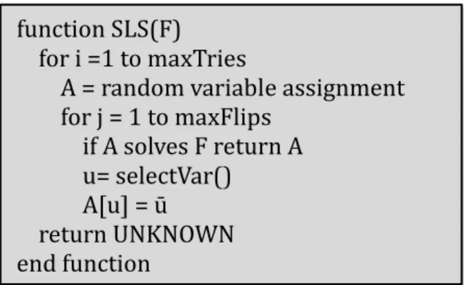
Incomplete solvers attempt to find a satisfying assignment when one exists. Typically there is no guarantee that one will be found. They are unable to declare formulae as being unsatisfiable. The vast majority of incomplete solvers come from the category of Stochastic Local Search (SLS). Many different SLS algorithms exist, and the vast majority of SLS solvers conform to the structure described in the pseudo code in Figure 2 where F represents the formula, A represents the current random assignment, and u represents the variable selected to flip.
The SLS algorithm is given a predetermined number of tries to find a solution to the formula. For each try the algorithm begins with a random assignment generated for each variable in the formula. From this random assignment each clause is determined to be satisfied or unsatisfied. Then, for a maximum number of flips a variable is selected and its assignment is flipped. The variation from one SLS solver to another is found in the technique for selecting the next variable to flip. If the SLS solver performs the
function SLS(F) for i =1 to maxTries
A = random variable assignment for j = 1 to maxFlips if A solves F return A u= selectVar() A[u] = u return UNKNOWN end function
maximum number of flips on all its tries without satisfying the formula, the solver returns unknown since it is unable to declare unsatisfiability.
The algorithm implemented in GSAT is a greedy hill-climbing approach to SLS [24]. GSAT begins with a randomly generated truth assignment. GSAT then flips the truth assignment of the literal that results in the largest decrease in the number of unsatisfied clauses. GSAT performs flips until a maximum number of flips is reached or a flip results in a satisfying assignment. It starts with a new randomly generated truth assignment and performs the flip procedure for a maximum number of tries. GSAT is very similar to the general implementation of a SLS solver. It however includes the concept of sideways moves. Sideways moves allow GSAT to perform flips to variables that do not increase the number of satisfied clauses. The implementation of sideways moves provides GSAT a strategy for escaping local minimum, which is often a struggle for greedy algorithms approaches. It can be shown that an SLS solver will not be able to find a solution unless it begins with an assignment that is very close to a satisfying assignment on some problem instances. Note that a wrong assignment for a single variable can lead the search to an unsatisfiable formula. Greedy algorithms may repeatedly select the same assignment for a variable, leading the search down the same path which may not be promising. GSAT’s implementation of sideways moves is a technique for solving this problem because it allows variable flips that are contradictory to the normal greedy strategy.
WalkSAT builds on GSAT by augmenting it with a random walk strategy [23]. The random walk strategy picks a variable from an unsatisfied clause and flips it thereby satisfying the selected clause. The randomness of the walk strategy is dependent on
probability p. The algorithm selects a random unsatisfied clause. Then with probability p,
the variable that will result in the largest decrease in the number of unsatisfied clauses is selected and flipped, as GSAT does. Otherwise, a random literal in the selected clause is selected and flipped. The number of flips performed is bounded by a maximum number of flips, and the number of tries with a new randomly generated truth assignment is bounded by a maximum number of tries. In Chapter 3, each reference to WalkSAT refers to the Java implementation found in the MiniSat library [14].
The 2007 SAT Competition Gold Medal winner in the random category,
gNovelty+, is an SLS solver building off concepts of previous SAT Competition winners [22]. The algorithm for gNovelty+ begins with a random assignment. Then for a max number of steps the algorithm determines if the current state is within the probability for walking. If so, a random variable is selected from a false clause and flipped. If not, a check is performed to see if a variable that if flipped will reduce the number of unsatisfied clauses, essentially reducing the formula size; such a variable is considered
promising variable. If a promising variable exists, select the least recently flipped promising variable. With no identified promising variables, a weighted objective function is used to select the next variable and the weight of all false clauses is increased by one. The algorithm for gNovelty+ includes weight smoothing probability when weights are increased, which for this case means that when false clause weights are updated, the weight of all clauses is reduced by one. This entire procedure can be restarted and completed for a maximum number of tries.
UnitWalk is a local search algorithm with a unique twist [12]. The main difference between UnitWalk and other SLS solvers is that UnitWalk modifies the
formula during the algorithm. Similar to most SLS solvers, the algorithm begins with a random assignment. UnitWalk then proceeds in periods and each period starts by generating a random permutation for the variables in the formula. This permutation dictates the order in which variables are picked during the period. Like DPLL, UnitWalk uses unit propagation to reduce the size of the formula during a period. First unit propagation is attempted; if a unit clause exists, the variable selected is the unit variable. If the current random assignment for the variable does not satisfy another unit clause, i.e., there is no conflict, then the variable’s truth value in the current random assignment is set to the value that would satisfy the unit clause. Note that this might entail flipping the variable’s value in the current random assignment. Once all the unit clauses are eliminated in this manner, the next variable is selected from the random permutation that was generated. If the variable was not already assigned by unit propagation, the variable is assigned the value in the current random assignment and unit propagation is invoked again. Once all the variables in the formula have been processed, if the formula is empty then it is declared to be satisfiable. Otherwise (a conflict occurred) if no variable was flipped during a period, then UnitWalk randomly flips one of the variables in the current assignment. This ends the current period and the formula is reset to the original formula for the next period. After a specified number of periods, search starts at a new random assignment.
2.4 Hybrid Solvers
Hybrid SAT solvers have become a prominent area of SAT solver research. Hybrid solvers have been shown to be effective in solving all three SAT formula families, namely, crafted, application, and random. A hybrid solver comprises two or
more SAT solvers. The hybridizing process varies from one hybrid solver to the next. The basic goal is to create a solver that inherits the strengths of each component solver without inheriting their corresponding weaknesses. An ideal solver is fast, complete, uses little memory, and fares well on all SAT formula families. SLS solvers are very good at solving problem instances from the random formula family and typically use little memory. DPLL solvers are very good at solving application and crafted problem instances, but they are very memory intensive and tend to perform poorly on the random formula family. Below we discuss some successful hybrid solvers from the literature.
A hybrid solver hybridGM [2] utilizes the SLS solver gNovelty+ and a DPLL solver March_ks [11]. The implementation of hybridGM uses SLS as the lead solver and DPLL periodically to help the lead solver, resulting in an incomplete solver. Having the SLS solver take the lead means that the solver begins with a complete random assignment. Then, for a predetermined number of flips a variable’s truth value is flipped. During the process of flipping variables a Search Space Partition (SSP) is constructed with the goal of studying local minimum and their neighborhoods. A local minimum exists when flipping a single variable will not solve the current conflict; rather multiple flips need to be made in order to move past the conflict. The goal of an SSP is to monitor the flips in the neighborhood of the local minimum to determine which variables are conflicting and unassign these variables. The partial assignment created by the SSP based on the random assignment and the unassigned and possibly conflicting values are passed to the DPLL solver when the SSP grows to a predetermined size. The DPLL solver may find an assignment for the unassigned variables in which case hybridGM returns the assignment. When the DPLL solver cannot find a satisfying assignment of the variables,
a solution to the conflict does not exist in the unassigned variables of the SSP. The SLS solver then continues to find another local minimum and tries the strategy again until a solution is found.
SatHys is a complete hybrid solver where the two solvers take equal advantage of each other [1]. SatHys aims to take advantage of research showing that local search algorithms can provide important information to a DPLL solver. In SatHys, the SLS solver is used to steer the DPLL solver towards proving unsatisfiability while the DPLL solver is used to direct the SLS solver to a solution, if one exists. The solver begins by first applying unit propagation to the original formula. Any variables assigned during unit propagation are stored in the current partial assignment. A complete assignment is generated by randomly assigning each of the variables outside of the partial assignment. The SLS solver is then called on the complete assignment. When the SLS algorithm is executed it performs normally by flipping variables to reduce the number of unsatisfied clauses. The SLS search is halted when a local minimum is reached and the activity values of the DPLL solver’s formula are updated according to the search conducted by the SLS solver. At this time the DPLL solver is used to select the next variable or another strategy such as rsaps [13] or novelty [20] is applied. It is noted that as long as the SLS solver allows for improvements it is favored to execute the SLS solver. The DPLL solver is invoked based on a value which measures how well the SLS solver is currently performing. This value is decreased every time the SLS solver reaches a local minimum. When the DPLL solver is called, a literal is selected based on the updated variable activities and the truth assignment is selected from the complete assignment generated by SLS which results in the largest number of satisfied clauses. When a restart occurs a new
complete assignment is generated. This procedure is performed until a satisfying assignment is found or the formula is determined to be unsatisfiable. According to the experiments presented in the paper, SatHys is a solver that does well on all three problem types: crafted, application, and random. Even though it is not the best for any formula family it performs close to the best and is able to perform well on all categories.
Another interesting approach is adopted by hybrid solver HBISAT (HyBrid Incremental SAT Solver), which again combines DPLL and local search [7]. In each iteration, local search attempts to find a satisfying assignment. If a solution is found, the solution is returned to HBISAT, validated and returned. Otherwise, local search is used to collect unsatisfied clauses. Note if DPLL determines this collection of unsatisfied clauses to be unsatisfiable, then the entire formula can be guaranteed unsatisfiable. If DPLL is able to find a satisfying assignment, the assignment is passed back to local search for the next iteration. Each iteration adds the set of unsatisfied clauses to a database of unique clauses. Eventually the database will contain the entire formula. In order to reduce the number of iterations before the clause database contains all clauses, HBISAT uses "clause padding". Clause padding adds clauses related to the unsatisfied clauses in a single iteration. This can help DPLL find unsatisfiability sooner as well as speed up incremental search. Related clauses are either clauses containing the most flipped variable or clauses with two or more variables with opposite polarities of literals contained in the broken clauses. The paper discusses using WalkSAT as its local search, however declares itself to be flexible to other solvers.
Chapter 3
AmbSAT: A Complete Hybrid Solver
In this chapter we describe our hybrid solver, AmbSAT. AmbSAT is a complete solver that uses the DPLL solver MiniSAT and the SLS solver WalkSAT. We chose AmbSAT, where Amb represents ambivalence, which is an essential notion in our solver. In upcoming sections we discuss basic concepts related to the solver, the decisions made as a part of implementing a hybrid solver, the notion of scout vs. leader, and the notion of ambivalence.
3.1 Basic Concepts
Overall, the implementation of AmbSAT attempts to combine an SLS and DPLL solver in such a way that utilizes the benefits of each solver without incurring a large amount of overhead.
In order to maintain the completeness of the DPLL algorithm, the hybridization technique exploited in AmbSAT is to have the SLS solver aid the DPLL solver in its decision making process. The exploration of AmbSAT is very similar to the traversal implemented by DPLL. The combination strategy used in AmbSAT is unique in comparison to existing hybrid solvers. AmbSAT utilizes an SLS solver periodically in place of using the branching heuristic in MiniSAT, where the results from the SLS solver are used to select the next variable.
The DPLL algorithm is referred to as the leader because it guides the search until it is determined that more information is required to continue. When more information is required, the SLS solver is invoked; the SLS solver is referred to as the scout since it goes
out and gathers information. The scout returns which clause it found the hardest to satisfy. The DPLL then selects a variable from this clause as the next branch variable.
Essential to the implementation of AmbSAT is our notion of ambivalence. This abstract notion of ambivalence aims to capture when exactly the leader may not have a clear preference for which branch variable to use at a search tree node. When ambivalence is detected, the scout is invoked to identify a difficult to satisfy clause. The added bonus of executing the scout is that the scout may find a solution, in which case the search is complete.
3.2 Designing for Efficiency
The MiniSAT implementation utilizes a max-heap to organize variables based on their activity values. At the beginning of a search, MiniSAT sets the activity values for all the variables in the formula to zero. The algorithm moves through the heap of variables, selecting one at a time until a conflict occurs. When a conflict occurs, the activity values of the variables involved in the conflict are incremented. Within AmbSAT, ambivalence is not computed until after the first conflict has occurred. However, the scout is invoked at the root node of the search tree with the intention of steering the leader in the right direction from the beginning of the search and giving the scout the opportunity to solve the problem quickly.
The computation involved for each specific notion of ambivalence presented in Section 3.6 requires access to some of the elements in the heap. Heap implementations include a pop method that removes the root element of the heap and reorganizes the heap to maintain heap properties. Performing the pop operation N times would result in a
collection of the largest N elements. Ordinarily the pop operation would suffice for the purpose of inspecting the variables stored in the heap. However, the N elements that were removed using the pop operation would need to be placed back into the heap. Simply inserting the elements back into the heap may result in a change of heap ordering when multiple variables have the same activity values. Since the ordering of the heap may be altered, the search path chosen by the leader may also change, which AmbSAT attempts to avoid. When the leader is not ambivalent, AmbSAT attempts to let the leader perform as it would have without the hybridization. For this reason, a peek function was implemented allowing the ability to access any element in the heap without removing the element from the heap. Less overhead time exists when utilizing the peek function implemented as opposed to performing pops and manipulating the heap.
MiniSAT implements a lazy heap management technique that allows the heap to contain both assigned and unassigned variables. During the branch variable selection process, MiniSAT removes assigned variables from the heap until an appropriate unassigned variable is found. Note that this does not ensure that the heap only contains unassigned variables once an unassigned variable is found. It is possible that the heap may contain assigned variables further down the heap.
Through the definition of a standard max-heap, it is known that in order to find the largest N items, the first 2N – 1 items must be accessed to determine the largest N
items. However, since the heap used for AmbSAT may contain assigned variables this definition becomes complicated. In order to find the true largest N items, it would have to be tracked how many assigned items are encountered on the heap and the number of checked items would have to be increased accordingly. Rather than incurring the
overhead of finding the true N largest elements, it was determined that an approximation was sufficient. In doing so, each type of ambivalence uses two parameters: the number of unassigned elements to check and N, the number of largest unassigned elements to obtain from the checked elements.
When the scout is invoked it is provided with a sub-problem of the original problem based on the current partial assignment generated by the leader. There are two benefits to allowing the scout to solve a sub-problem rather than the entire formula. The first is that the scout will find it easier to solver a smaller problem and if the scout is able to solve the sub-problem then the formula is satisfiable. The second is that AmbSAT seeks to extend the current partial assignment upon invocation of the scout. Hence, it is appropriate to give the scout a list of clauses that remain to be satisfied and a list of unassigned variables in those clauses to avoid obtaining data that is conflicting with the leader’s current partial assignment.
When supplying the scout with a sub-problem, all clauses that are left unsatisfied by the current partial assignment are included. For clauses that are unsatisfied but contain assigned literals, the clause is modified to provide only unassigned variables. AmbSAT uses an efficient technique for maintaining the set of unsatisfied clauses. The maintenance includes creation of an array to store the size of each clause in the formula and a two-dimensional array whose rows correspond to the clauses in the formula. This memory is allocated only once at the very beginning of a run when the two-dimensional array is created to store the original clauses in the formula and the size array is initialized to the original clause sizes. The implementation specifics for the setup of the clause and size arrays can be viewed in Figure 11 of Appendix E.
The clause set is not maintained every time a variable is assigned. Rather the clause set is updated prior to invoking the scout. Updating the clause set includes looping through each clause and adjusting accordingly. When the leader has satisfied the clause the size is set to zero in the size array. For each clause that remains in the formula, we process the clause variables in the following manner. Each clause variable that has an assigned value is moved to the end of the clause and the size of the clause is decremented by one. Figure 12 of Appendix E displays the implementation details of the clause maintenance method described here.
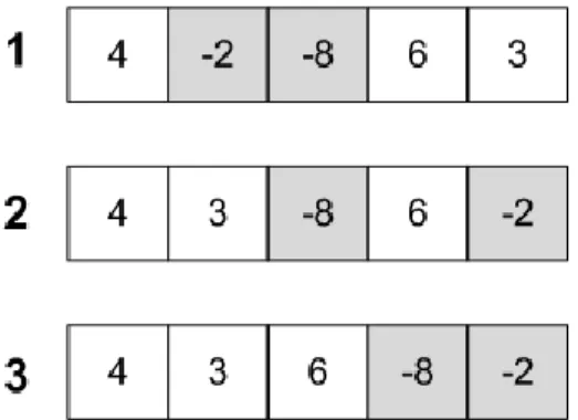
Figure 3 depicts the action of shifting assigned variables to the end of the clause array. In the figure the assigned variables are -2 and -8 represented by grayed out indices of the array. In step one, the original array is displayed and the first element encountered is the 4. Since literal 4 is unassigned no action is taken at this time. However, in step two you can see that the array has been altered. In this pass of the array -2 is encountered which is an assigned variable. Comparing step one to step two it can be observed that the -2 and 3 have swapped positions. At this time the size of the clause is also decremented
from five to four to adjust for the assigned variable in the clause. In the next pass the encountered element will be the 3, in its new position, and no action will occur since it is unassigned. With one more pass through the array all assigned variables will be moved to the end of the array when the -8 is encountered and swapped in position with the 6. Step three depicts the final clause array with the assigned variables appearing at the end of the clause and the clause size set to three, the number of unassigned variables.
Even with the enhancements made to reduce the amount of overhead based on the memory allocation, invoking the scout at every node incurs an excessive amount of overhead. It was determined that the scout should be called only when the leader indicates that it needs help. The notion of the leader requiring further guidance lead to the development of the notion of ambivalence for detecting situations where the branching heuristic is unsure of which variable to select next. Additionally, as discussed in the next section, AmbSAT caps the scout runtime overhead at a fixed percentage of its total runtime.
3.3 Experimentation Methodology
The problem set for these experiments comprises of 29 files collected from the 2005, 2007, 2009, and 2011 SAT competitions (see Appendix A). 4 The vast majority of the problem set consists of problem instances from the application and crafted SAT formula families. As will be evident from our results, AmbSAT’s performance on the random SAT formula family is vastly superior to MiniSAT’s performance, so our problem set only includes two files belonging to the random SAT formula family. Therefore, our results compare AmbSAT’s performance with the performance of
MiniSAT for formulae that MiniSAT is known to excel at solving. The problem set was used to establish parameter settings that are applied to all ambivalence notions as well as parameters that pertain to specific ambivalence notions. The problem set was initially run on MiniSAT in order to allow comparisons of each ambivalence notion implementation. Appendix B displays the time and node count performance recorded by MiniSAT. Future paragraphs of this section discuss the parameters that are common to all notions of ambivalence. Section 3.6 presents specific ambivalence notions and experimental results thereof.
In Section 3.6 we will describe several implementations of AmbSAT that vary based on their specific notion of ambivalence as well as the choice of parameter settings. Since all implementations use a probabilistic SLS solver, we run each solver three times on the problem set in order to help understand its performance in the average case, as well as the influence of various parameter settings. When analyzing the results of various parameter settings, AmbSAT’s run time performance is compared to MiniSAT’s run time performance. When two or more settings returned similar results based on time, the number of nodes expanded in MiniSAT’s tree is used as the secondary comparison characteristic.
Parameters were optimized using a binary search-like technique, whereby a couple starting values were selected and the values were adjusted higher, lower, or in the middle of the starting values based on the run results. For instance, when finding a setting for normalized percentage ambivalence, discussed in Section 3.6.3, values between 0 and 1 were initially run with increments of 0.1. A run was conducted on a short subset of the problem set for use in selecting values which seemed to be the most promising. The
results indicated that values on the lower end of the spectrum appeared to be the most promising. With some more data, we were able to detect that the values 0.1 and 0.2 performed the best regularly. So, then the binary search strategy used suggested runs on values between 0.05 and 0.25. This binary search strategy then was applied on smaller values in the ranges that seemed promising resulting in runs with values such as 0.11 and 0.125. Multiple promising values were selected based on the binary search strategy and executed on the 29 file problem set. The graphs in the upcoming sections present the percentage of files in the problem set where AmbSAT performs better than MiniSAT. In the graph related to each ambivalence notion, the selected parameter settings are displayed compared to a setting numerically less than the selected value and a setting numerically greater than the selected value.
3.4 Design Settings
One important consideration in AmbSAT’s design was the issue of overhead incurred by the scout invocations. Clearly, if the overhead grows too large it cannot possibly compete with MiniSAT. On the other hand, it is desirable to have the scout to be called a sufficient number of times so AmbSAT can gain the benefits of the scout invocation. To do this, AmbSAT keeps track of the number of times ambivalence is detected and the total amount of time the scout runs have taken so far. Another scout invocation can only be made when the amount of scout time so far plus the estimated amount of time for one more scout invocation is less than the predetermined percentage overhead allowed. The average scout run time is estimated from past scout run times.
Figure 4 displays the results of each of the three runs where the scout overhead percentage is limited to 2.5%, 5%, and 7.5% respectively. Section 3.6.3 discusses AmbSAT’s implementation of Normalized Percentage Ambivalence with percentage 0.125 that was used to produce the data displayed in Figure 4. The selected setting for the percentage overhead is 5%. Appendix C displays the detailed time and node count performance based on 5% overhead. Although all three settings perform fairly well against the MiniSAT implementation, consistency is a key deciding factor. It can be seen that the center set of bars for each of the three runs is about 55%. Although a single 2.5% run performs better than the best 5% run, the other two runs perform worse than the worst 5% run. It can be seen that the variation from run to run is larger than with 5% overhead. Run 3 of the 7.5% overhead runs performs as well as the first two runs at 5%, but the other two runs perform significantly worse.
0% 10% 20% 30% 40% 50% 60% 70% 2.50% 5.00% 7.50% Am bSAT Fa st er Tha n M in iSAT Run 1 Run 2 Run 3
Figure 4 Performance of AmbSAT with Different Allowable Overhead Percentages vs. MiniSAT
Once it is determined how and when to call the scout, it needs to be determined how to use the scout to benefit the decision making process of the leader. We decided to use the scout to find out the clause that seems the hardest to satisfy and convey this information to the leader. The leader can then assign an unassigned variable in this clause in a manner to satisfy the clause. The scout keeps track of how many times each clause is unsatisfied with the different assignments that it explores. When the scout completes its traversal without satisfying the sub-problem, it returns the clause number that has the most unsatisfied count. From this clause, the leader selects the unassigned variable with the largest activity value.
It is possible that the clause selected by the scout may be made up of all unassigned variables without an activity value. Recall that a variable’s activity value is incremented only when it is involved in a conflict. Therefore, it may be that the variables remaining in the selected clause have not occurred in a conflict, thus having an activity value of 0. In this case, there needs to be a technique for selecting a variable from this clause. To handle this case, three strategies were defined:
1. Random Selection – The most basic technique for variable selection includes randomly selecting an unassigned variable in the clause.
2. Variable Count Selection – A slightly more complex technique for variable selection which includes selecting the variable which appears most in the unsatisfied clauses in either its positive or negative polarity.
similar to the Variable Count Selection strategy. The difference is that this technique selects the variable which occurs most in unsatisfied clauses in the polarity that it appears in the selected clause.
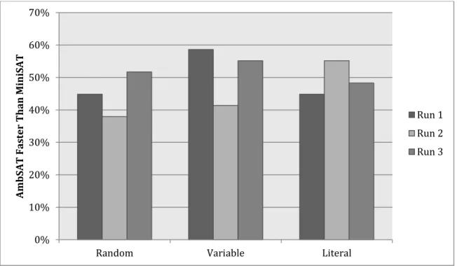
Figure 5 Performance of AmbSAT Selection Strategies vs. MiniSAT
Figure 5 displays the results comparing the different possible selection strategies used to select a variable in a clause where the unassigned variables have activity values of zero. The data displayed in
Figure 5 was produced with AmbSAT’s implementation of Normalized Percentage Ambivalence with percentage 0.125, discussed in Section 3.6.3. The Variable Count selection strategy is determined to be the lowest performing strategy because of the large amount of variation from run to run. Although this strategy has the largest
0% 10% 20% 30% 40% 50% 60% 70%
Random Variable Literal
AmbS AT Fa st er Th an Mi niSAT Run 1 Run 2 Run 3
percentage two of the three runs, the variance from smallest to largest percentage is 17%. From the data presented and based on the elimination of variable selection, the literal selection strategy is the selected setting because although it does not always perform the best, it performs the most consistent from one run to another. Literal selection is chosen over the random selection strategy based on the comparison of the two strategies showing that on both Run 1 and Run 3 the strategies perform equally or very close to each other. However, on Run 2 there is a large difference between the two strategies, in which literal selection is the clear superior. Appendix D displays the detailed results pertaining to the selection of literal selection as the selection strategy.
3.5 Implementation Details
In designing and implementing AmbSAT, it was a goal to develop a solver that modified the component solvers used as little as possible. In order to accomplish this goal, AmbSAT is implemented in such a way that uses MiniSAT and WalkSAT in their original implementation states. It should be noted that the only code modified within MiniSAT’s implementation is an addition of a method to each clause type returning the clause in an integer array for use with the sub-problem clause set. Although the C implementation of WalkSAT utilizes the clause and size array the Java implementation did not, modifications were made to the Java implementation to more closely match the C implementation with the inclusion of these two arrays.
The process of executing AmbSAT begins with its own launcher class, adapted from a basic launcher of MiniSAT. The launcher class is responsible for setting up AmbSAT to run with user specified parameters as well as invoking methods to read the
problem formula and start the search process. Since the goal of AmbSAT is to allow MiniSAT to perform a regular search procedure until a state of ambivalence is detected, most of the setup procedure is exactly what would be performed to execute MiniSAT. In addition to initializing MiniSAT’s default solver, reading the problem formula, and starting the search, AmbSAT also loads user specified parameters for notions of ambivalence, percentage overhead, and selection strategy as well as initializing the clause and size arrays for use when passing a sub-problem to WalkSAT.
The use of MiniSAT’s variable heap is important in the implementation of AmbSAT. In order to allow AmbSAT to function independently from MiniSAT, AmbSAT sets the MiniSAT default solver to use a heap within AmbSAT. The heap developed is based on the variable heap used by MiniSAT. AmbSAT’s heap includes the addition of two methods used to maintain the clause set for WalkSAT’s problem. The first method is used to initialize the clause and size arrays to store the original clauses and clause sizes. The second method is used to modify the ordering of the variables in the clause array to have assigned variables at the end of the array and the clause size reduced, as discussed in Section 3.2. Lastly, the select method is modified to handle checking for ambivalence and invoking WalkSAT when ambivalence is detected. Figure 6 displays the pseudo code for the modified select method. The actual code for the select method, sub-problem clause initialization, and sub-sub-problem clause maintenance can be found in Appendix E.
Figure 6 displays the heap’s select operation where a variable is either selected from the heap using traditional MiniSAT strategies, or selected based on data returned by a call to WalkSAT. The lines displayed with bolded text are the portions of the select
method that are added for AmbSAT’s combination of MiniSAT with WalkSAT. Performing just as MiniSAT does, first it is checked that the heap is not empty. Then, variable V is selected as the first variable in the heap. The only change in variable V is that in AmbSAT’s select method the first element is retrieved through a peek method as opposed to the pop method used by MiniSAT. Since MiniSAT uses a lazy strategy for heap maintenance, we first check if the variable has been assigned. If the variable is unassigned, proceed by checking for ambivalence. Otherwise simply remove the assigned variable from the heap. Ambivalence is checked according the specific notion of
function select ( )
while (heap is not empty) V = first heap element if (V is unassigned)
if (ambivalent)
Build sub-problem, S, with unsatisfied clauses and variables satisfied = Invoke WalkSAT on S
if (satisfied)
return SATISFIABLE C = WalkSAT’s hardest clause
V’ = Invoke selection strategy to select variable in C
remove V’ from heap return V’
else
remove V from heap end while
return UNDEFINED end function select
ambivalence that is specified in the code. If ambivalence is detected, the sub-problem clauses are updated and WalkSAT is invoked on the sub-problem. If WalkSAT is successful in finding a solution to the formula, the search is complete. When WalkSAT does not solve the sub-problem, it returns the clause that was the hardest to satisfy during it search. This hardest clause is passed to the selection strategy, which returns an unassigned variable, V’, in the clause. When possible, the selection strategy picks an assigned variable that has the largest activity value. If all unassigned variables in the selected clause have a zero activity value, the selection strategy applies its unique technique to select one of the unassigned variables. The selected variable is applied as the next branch variable, and the polarity is selected to satisfy the clause. The selected variable is removed from the heap and returned for assignment to reduce the size of the formula.
The heap’s select method relies on two other implementations: selection strategy, and ambivalence. First, the implementation details of the selection strategies are discussed. The three different selection strategies were discussed in Section 3.4 with results pertaining to each setting. The three strategies are random, variable count, and literal count. Random selects a random unassigned variable in the clause selected by WalkSAT. Variable count selects the variable that appears in the most unsatisfied clauses in either polarity. Literal count selects the variable that appears in the most unsatisfied clauses in the polarity it appears in the selected clause. Conceptually the strategies are not very complex. The resulting implementation is also very simple. Random selection is basic, generating a random number between 0 and the number of unassigned variables in the clause, and selecting the variable at the generated position. The variable count and
literal count selection algorithms utilize a list of counts maintained by WalkSAT. This count collection allows these selection strategies to be implemented in an efficient manner.
The unique notion of ambivalence implemented in AmbSAT is the key to its success displayed through data in Section 3.6. Different implementations of ambivalence rely on the creativity to develop a notion of ambivalence. Different notions share the same common goal, but the implementations vary from one to another. A single notion is abstracted into its own class where the Chain of Responsibility (COR) design pattern is used to allow one notion to contain another notion [25]. This design pattern allows implementation of the chain of command so that multiple notions of ambivalence can interact with one another.
Ambivalence is implemented as an abstract class containing an Ambivalence object and an abstract method to determine ambivalence. The implementation of abstract Ambivalence class can be found in Figure 13 of Appendix F. Each specific notion of ambivalence defines the method to determine ambivalence according to the specifics of its notion. The use of COR allows notions of ambivalence to function as a chain of procedures. The chain requires the current ambivalence notion to declare ambivalence before another notion is evaluated. Each notion of ambivalence in the chain must declare ambivalence for the leader to be declared ambivalent. When a single notion of ambivalence does not declare ambivalence, the evaluation is terminated. For instance in the implementation of AmbSAT, if the overhead is not under the 5% limit then further notions of ambivalence will not be evaluated. For this reason, it is most logical to apply the least costly, in terms of overhead time, first so if ambivalence is going to return false