Reduction of Power and Virtual Machine Migration Inside a Cloud Datacenter

(1)

REDUCTION OF POWER AND VIRTUAL MACHINE MIGRATION INSIDE A CLOUD DATACENTER

A Thesis in

Electrical Engineering

Presented to the Faculty of the University of Missouri–Kansas City in partial fulfillment of

the requirements for the degree MASTER OF SCIENCE

by

AMARNATH BEEDIMANE HANUMANTHARAYA

B. E., Visvesvaraya Technological University, Karnataka, India, 2012

Kansas City, Missouri 2016

(2)

c

2016

(3)

REDUCTION OF POWER AND VIRTUAL MACHINE MIGRATION INSIDE A CLOUD DATACENTER

Amarnath Beedimane Hanumantharaya, Candidate for the Master of Science Degree University of Missouri–Kansas City, 2016

ABSTRACT

Today’s datacenter consumes high amount of electrical energy for its operation. It increases day by day, thus increasing the operation cost and carbon dioxide emission. To reduce the power consumption at a datacenter, a model with an adaptive threshold virtual machine (VM) consolidation method that reduces the number of VM migration and power consumption in the datacenter was used. By consolidating VMs and switching off unused hosts, a cloud provider can reduce physical resource usage and power consumption. But due to service level agreement(SLA) between a cloud service provider and cloud users, a cloud service provider cannot degrade the performance. To balance between energy and performance, a cloud service provider must maintain a reasonable performance while reducing power consumption. In this thesis work a novel technique have been proposed to adhere both power and performance by implementing an adaptive host upper utilization

(4)

our model more robust than the existing models. Our proposed algorithm reduces the power consumption and limits the number of VM migration while ensuring high level of SLA. To simulate the experiment and to validate our proposed algorithm using real world datacenter datasets, we have used CloudSim which is a widely popular datacenter simulation toolkit.

(5)

APPROVAL PAGE

The faculty listed below, appointed by the Dean of the School of Computing and En-gineering, have examined a thesis titled “Reduction of Power and Virtual Machine mi-gration Inside a Cloud Datacenter,” presented by Amarnath Beedimane Hanumantharaya, candidate for the Master of Science degree, and certify that in their opinion it is worthy of acceptance.

Supervisory Committee

Dr. Deep Medhi, Ph.D., Committee Chair

Department of Computer Science & Electrical Engineering Dr. Cory Beard, Ph.D.

Department of Computer Science & Electrical Engineering Dr. Sejun Song, Ph.D.

(6)

CONTENTS ABSTRACT . . . iii ILLUSTRATIONS . . . viii TABLES . . . xi ACKNOWLEDGEMENTS . . . xii Chapter 1 INTRODUCTION . . . 1

1.1 Motivation For The Work . . . 3

1.2 Objective Of The Work . . . 3

1.3 Summary Of Contributions . . . 3

1.4 Organization . . . 4

2 LITERATURE SURVEY . . . 5

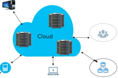
3 CLOUD COMPUTING . . . 8

3.1 Cloud Computing Architecture . . . 8

3.2 Deployment Models . . . 8

3.3 Cloud Computing Properties . . . 9

3.4 Service Models . . . 10

3.5 Security And Privacy . . . 11

3.6 Disadvantages Of Cloud Computing . . . 12

(7)

4.1 Introduction To Cloudsim . . . 13

4.2 Design And Implementation Of Cloudsim . . . 13

4.3 System Model . . . 16

5 MODELS . . . 21

5.1 Host Overloading Detection . . . 21

5.2 VM Selection Policy . . . 24

5.3 Host Underloading Detection and Host Overloading Detection . . . 25

5.4 VM Placement in Cloudsim . . . 27

6 RESULT . . . 29

6.1 Simulation Setup . . . 29

6.2 Simulation Result And Analysis . . . 31

7 CONCLUSION . . . 44

Appendix A Information . . . 45

A.1 Workload Pattern . . . 45

A.2 Number of VM migration . . . 47

A.3 Frequency of VM migration . . . 59

REFERENCE LIST . . . 61

(8)

ILLUSTRATIONS

Figure Page

1 Cloud Computing Model . . . 10

2 Cloudsim Class Design Diagram [6] . . . 14

3 System Model [6] . . . 17

4 Planetlab Data Results For Upper Threshold. . . 33

5 Selecting Optimum Value . . . 34

6 Planetlab Data Results For Upper Threshold And Lower Threshold After Selecting Optimum Value. . . 35

7 UMKC Data Results For Upper Threshold. . . 37

9 UMKC Data Results For Upper Threshold And Lower Threshold After Selecting Optimum Value. . . 39

10 Google Data Results For Upper Threshold. . . 41

12 Google Data Results For Upper Threshold And Lower Threshold After Selecting Optimum Value. . . 43

13 Panetlab Workload Pattern . . . 45

14 UMKC Workload Pattern . . . 46

(9)

16 Planetlab VM migration for VM 792 IQR model . . . 48

17 Planetlab VM migration for VM 1012 PTMA model . . . 48

18 Planetlab VM migration for VM 844 LR model . . . 49

19 Planetlab VM migration for VM 844 LRR model . . . 49

20 Planetlab VM migration for VM 987 MAD model . . . 50

21 Planetlab VM migration for VM 824 THR model . . . 50

22 Planetlab VM migration for VM 1012 for all the models . . . 51

23 UMKC VM migration for VM 488 IQR model . . . 52

24 UMKC VM migration for VM 305 PTMA model . . . 52

25 UMKC VM migration for VM 399 LR model . . . 53

26 UMKC VM migration for VM 399 LRR model . . . 53

27 UMKC VM migration for VM 453 MAD model . . . 54

28 UMKC VM migration for VM 225 THR model . . . 54

29 UMKC VM migration for VM 308 for all the models . . . 55

30 Google VM migration for VM 942 IQR model . . . 55

31 Google VM migration for VM 218 PTMA model . . . 56

32 Google VM migration for VM 943 LR model . . . 56

33 Google VM migration for VM 943 LRR model . . . 57

34 Google VM migration for VM 845 MAD model . . . 57

35 Google VM migration for VM 265 THR model . . . 58

36 Google VM migration for VM 218 for all the models . . . 58

(10)

38 VM migrations for UMKC data . . . 60 39 VM migrations for Google data . . . 60

(11)

TABLES

Tables Page

1 Cloud computing architecture. . . 8

2 Power consumption by the selected servers at different load levels in Watts [6] . . . 19

3 HP ProLiant ML110 G4 configuration. . . 29

4 HP ProLiant ML110 G5 configuration. . . 30

5 Virtual Machine’s Configuration. . . 30

6 Planetlab data result for upper threshold . . . 32

7 Planetlab data result for upper threshold and lower threshold . . . 34

8 UMKC data result for upper threshold . . . 36

9 UMKC data result for upper threshold and lower threshold . . . 38

10 Google data result for upper threshold . . . 40

(12)

ACKNOWLEDGEMENTS

I would like to thank my academic adviser Dr Deep Medhi for providing me an opportunity and helping along the way to complete my thesis work.

I would like to thank my parents, Hanumantharaya B and Krishnaveni, friends and family for making this happen.

I would like to thank University of Missouri - Kansas city for providing me an opportunity to work on this thesis report.

(13)

CHAPTER 1 INTRODUCTION

According to NIST, cloud computing is a model for enabling ubiquitous, on-demand access to a shared pool of configurable computing resources (e.g., computer net-works, servers, storage, applications and services), which can be rapidly provisioned and released with minimal management effort [16]. Cloud computing is mainly comprised of virtual machines and hosts, where a virtual machine emulates the operating system or application with full functionality of a given system and a host is nothing but a physical system or application. There are mainly three types of services offered by cloud comput-ing. They are Software as a service (SaaS), Platform as a service (PaaS) and Infrastructure as a service (IaaS). In this thesis, we address infrastructure as a service, which provides users with computing resources such as servers, networks, storages to complete their re-quired tasks. All these resources are provided to the user on a pay-as-you-go-basis, thus reducing the upfront cost in setting up the infrastructure to do the computation for the users. Moreover you can scale the physical hardware up or down depending upon your needs. Due to the narrow dynamic power range of the servers, the power consumption of an idle server is 60-80 % of their peak values [11]. These physical hardware consumes enormous amount of electrical energy to run, thus increasing the datacenter power us-age. It is estimated that datacenter electricity consumption is expected increase roughly by 140 billion kilowatt hours annually by 2020 in America alone [6] . Increase in power

(14)

consumption leads to increasing in carbon-di-oxide emission, thus contributing to green house gases.

Cloud datacenters are mainly dependent on server virtuliazation. Server virtual-ization is a technology in which physical resources are divided into a number of virtual machines, where the property of the virtual machines is same as that of physical chines. Server virtualization enables to distribute the workload among the virtual ma-chines, which are consolidated by a single physical machine, but also enables the tech-niques of virtual machine migration(VMM), which is a process of dynamically moving VM’s from one physical machine to another physical machine. VM migration has many benefits such as workload consolidation, load balancing, reducing energy consumption, facilitating maintenance activities as well as supporting mobile applications. There are certain challenges pertaining to VM migration such as related to service disruption, band-width consumption, management overhead, and increased security risks [5].

To reduce the operational cost a cloud service provider can degrade the perfor-mance of the systems but there is also a degradation of quality of service measured by service level agreement between the cloud service provider and cloud users. Degradation of service results in poor quality that could lead to reduction in the number of cloud users for that particular cloud service provider. Due to competition among the cloud service providers in the market, it is critical them to provide highest possible level of quality of service.

(15)

1.1 Motivation For The Work

Due to virtualization of computer systems, the use of servers has increased day by days thus contributing to the increase in power usage and bandwidth requirement by the datacenters which increasing the operating cost of the datacenter, carbon-di-oxide emis-sion and contribution towards global warming. There are several models which already exist but they are not optimized for balancing the power and giving the required Qos.

1.2 Objective Of The Work

The Objective of this thesis is to reduce the power consumption by limiting the VM migration and by turning off hosts based on a threshold and, thus increasing the residual bandwidth of network in the datacenter with minimum violation of service level agreement(SLA). We analyse and study the results obtained by simulating the datacenter operations by loading real life virtual machine’s historical cpu utilization data.

1.3 Summary Of Contributions

The main contributions of this work are:

• A new model is proposed to tackle power consumption and residual bandwidth inside a datacenter considering SLA violation into account.

• This new model consist of two types of detection methods. One is host overloading detection method and the other is host underloading detection method.

(16)

• Different models is compared with the proposed model to shown the that proposed model is better than the existing model.

1.4 Organization

The thesis is organized as follows: Chapter 2 present a literature survey on existing work on allocation policies, power and how those policies are different from our work. In chapter 3, we give an overview of cloud computing. In chapter 4 we discuss cloudsim, a simulation tool used in our work. In chapter 5 we discuss various existing models and proposes a new model for host upper and host lower threshold. In chapter 6, cloudsim setup and result are explained. In chapter 7, A conclusion about our work, drawbacks and limitation have been discussed.

(17)

CHAPTER 2 LITERATURE SURVEY

Cloud computing has become the starting point for those who do not want to buy, build and maintain computing resources as well as the applications and dipose of them when a job has been done [2, 21, 24]. Different VMs are provisioned and migrated according to customers needs [21]. A static consolidation method is not a viable option when you are choosing a live migration of VMs. Since, a static initial mapping, the consolidation of server are not done for a long time. A dynamic consolidation of VM’s is a better option [4]. Live VM migration help in turning off hosts as and when the hosts are under loaded, over loaded or both, thus minimizing the power consumption.

First work on power management regarding the virtualized datacenter has been proposed by Nathuji and schwan [19]. In this work, authors have proposed an archi-tecture relating to the datacenter. The archiarchi-tecture is division of resource management into local policies and global policies. At local level system borrows the guest operat-ing systems(OSs) power management strategies. At global level, information form the local managers is collected about the current resource allocation and decides whether the VM placement is needed. But the author has not specified a policy on how the automatic resource should be allocated at global level.

(18)

aware load balancing strategy. This policy is applied on VM with lower and upper thresh-old. If the load is greater or lower than the threshold, migration takes place. This exper-iment is carried out on 100 virtual machines and on 100 VMs. Here the authors do not consider the CPU utilization and real datacenter data for running their experiment.

A similar work has been conducted by Fahimeh et al. [12] that uses a K-nearest neighbour regression algorithm to predict resource usage in each host. Authors do not to give information on the number of VM migrations for the above mentioned algorithm since this is the crucial part of datacenter for deciding availability of residual bandwidth.

A similar work also been done by Girish et all [17]. In their work, they explored worked on upper and lower threshold to minimize the power consumption of datacenter and vm migrations. They proposed a formula for upper threshold and a static value of 30% for lower threshold. Since they were using a static value, it is not a good solution in ever increasing CPU utilization and dynamic workload of data inside the datacenter. Also, their work is on10hosts and20VM’s. While our work is based up on the dynamic value, this changes based on the cpu utilization.

VMware Vsphere distributed power management [1] operates on lower and upper utilization threshold which is set at45%and81%, respectively. This is not a good practice since the utilization value may vary differently for different datacenters.

Rajkumar and Anton [3] have proposed a novel technique, which deal with the problem of power and efficient dynamic consolidation of vm. Authors have proposed var-ious host overloading detection algorithms but there is only a general host under loading

(19)

detection algorithm. In our work we not only specify the policy for host over loading de-tection but also to the host under loading dede-tection, thus reducing the power consumption, over-all SLA violation and reducing the number of VM migrations which intern increase in the residual bandwidth of the datacenter.

Power reduction can also be done by VM consolidation. Shingo and Toshhinori has proposed a rank based VM consolidation method [26]. Migration of VM to destina-tion host is selected on a host rank basis, where Rank is assigned to the server on basis of whether the server models are new or old which is decided by the datacenter operator. This is an added work to datacenter operator.

(20)

CHAPTER 3 CLOUD COMPUTING

3.1 Cloud Computing Architecture

The basic Cloud computing architecture is divided in to six kinds as follows: Clients Here end user are considered clients like web browser or an apps; Services

-Table 1: Cloud computing architecture. Clients Services Application Platforms Storage Infrastructure

Function in clouds; Application - backbone of service; Platforms - A base for develop-ing, running and managing cloud application; Storage - Storage of data in remote server; Infrastructure- Provides virtualized computing resource.

3.2 Deployment Models

There are four different types of cloud services provided by a cloud service provider and they are:

1. Public cloud - A cloud which is open for public use and may be owned, managed, operated by business, academic, or government organizations or their combinations and

(21)

usually operates on premises of cloud providers.

2. Private cloud - These type of clouds is provided for exclusive use of a single organiza-tion and may be owned, managed and operated by an organizaorganiza-tion, a third party or their combination and usually operates on or off the organizations premises

3. Community cloud - Exclusive use by a community, for example, federal government initiative for various government services and may be owned, managed and operated by organization, a third party or their combinations. This may operate on or off the organi-zations premises.

4. Hybrid cloud - It is a combination of above distinct cloud infrastructures but bound together by standardized or propriety technology for portability and translate fixed cost in to fixed and variable cost.

3.3 Cloud Computing Properties

Some of the Cloud inside the properties:

• Scalability

• Resource pooling, aka multi-tenancy

• Migration of task and data

• measured/monitored/audited resource usage

(22)

Some of the user visible properties:

• On demand

• Self service

• Rapid elasticity

• Broad network access

• User visible service agreement

• pay as you go model

3.4 Service Models

Cloud computing offers services mainly in three different categories. They are Infrastructure, Software and Platform as a service.

(23)

1. Software as a service(Saas) - Software’s is provided by an on demand delivery model, which means software licensing are provided on a subscription basis. A common delivery model is used to provide the business application, office, HR application, Anti virus software etc. some of the examples include office 365, Google docs, Gmail, Hotmail etc.

2. Platform as a service(PaaS) - Platform as a service provides a platform for entire app development such as to develop, run and manage application without implementing infrastructure which is associated with developing and launching the app. Some of the examples are Google App engine, Windows Azure, Vmware Foundry, Heroku, Salesforce etc

3. Infrastructure as a service(IaaS) - Is a service that provide viritualized com-puting resources such as compute, storage and networks. It provides choices of virtual machines to install on bare metal machines. Some of the examples related to Iaas are Amazon Ec2, Vmware vCloud, Rackspace, Azure etc.

3.5 Security And Privacy

Cloud computing has several security and privacy issues because the service provider can access the user data, which is stored in cloud intentionally or unintentionally, can modify or even delete the data. Sometimes they can sell it to the third party which is already there in terms and conditions while users sign up for the services [25].

According to Cloud Security Alliance there are threats which are classified as top-most in cloud industries. They are Insecure Interfaces and API’s, Data Loss & Leakage,

(24)

and Hardware Failure which accounts for 29 % 25% and 10% of all cloud security issues. Since a cloud provider platform is being shared by different users their data is stored in the same data server. Therefore, there is a chances of information leakage of one user with other user [7]. The popularity of cloud computing has lead to Hyperjacking. Hy-perjacking is a kind of an attack where a hacker takes malicious control over the hyper visor that creates a virtual environment within an virtual machine. For example, Dropbox security breach which happened around October 2014 involved stealing of 7 million user passwords. Another problem with respect to cloud computing is the legal ownership of the data. According to [14], many terms and agreement are silent on the ownership of the data.

3.6 Disadvantages Of Cloud Computing

Cloud computing is an advantage in many way but there are several disadvantages. Number one being Downtime.Also No service provider can provide 100% immunity to-wards outages as cloud is completely dependent on internet connection. Since wear and tare may occur there is also hardware failure which is not in control of service provider. Cloud service provider may impose control on what cloud user can do while deploying the cloud, control and management of applications, data they can use or service they provide. Thus, there is a limited control over cloud from a cloud user perspective.

(25)

CHAPTER 4 CLOUDSIM

Cloudsim is a project by Clouds lab at University of Melbourne, Australia [6]. It is released as Open Source toolkit software under the Apache Version 2.0 license. This simulation toolkit was developed to perform repeatable and controlled experiments on services which users are working on, this to cut cost and to fine tune the performance before deploying in the real cloud. The Cloudsim version that use in our work is 3.0.3.

4.1 Introduction To Cloudsim

Some of the main features offered by Cloudsim are: support for simulation and modeling of large scale datacenters, energy-aware computational resource, datacenter net-work topology, pause and resume of simulation, insertion of simulation entities, and latest release support for application container.

4.2 Design And Implementation Of Cloudsim

Cloudsim contains certain fundamental classes which are the building blocsk of the Cloudsim toolkit. Below are the following classes:

• BwProvisioner: This class allows the cloud system developer and researcher to extend, according to their own policies. This class is an abstract class. The primary function of this class is to model the policy for provisioning of bandwidth to vm’s.

(26)

Figure 2: Cloudsim Class Design Diagram [6]

User’s can define the BW according to their usage. Which should be limited to the total available BW of the host.

• Cloudlet: Cloudlet are nothing but task. This class models the cloud-based applica-tion as a task to be executed like content delivery, social networking and business workflow. This takes input value in bytes.

• CloudletScheduler: This is a abstract class which defines how the processing power has to be shared. There are two kinds of provisioning policies they are space shared and time shared policies.

• Datacenter: This class models the core infrastructure level services that are offered by cloud service provider. It comprises of hardware’s such as memory, cpu cores, BW capacity and storage and contains a set of provisioning these components.

(27)

• DatacenterBroker:

• Datacenter broker is a mediator between software as a service and cloud provider. The user submit the number of cloudlet. and the broker submit the number of vm required to the datacenter.

• DatacenterCharecteristics: This class describes the basic configuration information of datacenter.

• Host: The host is nothing but the physical server or physical storage. This class contains the information like, what should be the ram size, BW, memory size, pes. vm selection policy, RAM and BW provisioner.

• NetworkTopology: This class contains the information on network topology which is produced by the BRITE topology.

• RamProvisioner: This abstract class allows deployment of vm in the host. Only if the Ram requirement is met. i.e only if the host has available ram. If not, it simply rejects the host.

• SanStorage: This class represents the large storage area of the datacenter like ama-zon EC3, Azure blob storage. Accessing the file in this storage require additional delay to show that there is a delay in transferring the data file.

• VM: Virtual machine class stores the information related to accessible memory, processor, storage size and vm internal provisioning policy.

(28)

• VmmAllocationPolicy: This class represent the provisioning of vm to the host. The main functionality of this is to select the host which has memory, storage, pes required by the vm.

• VMScheduler: Is an abstract class which models either the time shared or space shared allocation of pes to the vm.

4.3 System Model

In this study we consider an Infrastructure as a Service environment which is rep-resented by a large scale data center consisting of N heterogeneous physical nodes. These physical nodes are represented by i and having CPU performance defined by million in-structions per second(MIPS), amount of RAM and interface bandwidth. These nodes do not have local disks but storage is provided by a Network attached storage(NAS) to facilitate live VM migration across the servers. This type of environment is defined by no knowledge of application workload running on servers nor time required to provision the servers. Multiple independent users can submit requests for provisioning of M het-erogeneous VMs, characterized by requirements for processing power defined in MIPS, amount of RAM and network bandwidth. The fact is VMs are managed by sole users resulting in workloads created, which is combination of various applications such as HPC and web applications that utilize resources simultaneously. The user creates the SLA that formalizes the Quality of service delivery. The service provider may pay a penalty for any SLA violation.

(29)

Figure 3: System Model [6]

global manager as shown in Fig. 3. The local manager resides on each node as a module of VMM. Its function is to monitor the node CPU utilization, to re-size the VMs according to their resource needs, and to decide when and which VMs should be migrated from the node. The global manager resides on top of the master node and collects information from the local managers to maintain the overall view of the utilization of resources. The global manager issues commands for the optimization of the VM placement. VMMs perform actual re-sizing and migration of VMs as well as changes in power modes of the nodes [6].

4.3.1 Multi-core Architecture

Cloudsim is designed to consist of physical servers with multi core CPU’s. Each CPU is made up of n cores each core having m number of MIPS, thus making total processing power ofnmMIPS. This explains that application and VMs are not tied down to a single core but can be executed on an arbitrary core using time shared scheduling algorithm. The only limitation with this is that CPU capacity must be less than or equal to the capacity of a single core. This implies that if the CPU capacity required for VM is

(30)

higher than the capacity of a single core then VM must be executed on more than a single core. This is not a feasible situation.

4.3.2 Power Model

According to [18] power consumption by computing nodes in a datacenter is mostly determined by the CPU, disk storage, memory, power supplies and cooling sys-tems. Power consumption of a server can be accurately described by a linear relationship between power consumption and CPU utilization according to the study conducted by Fan X et all [11]. The simulations which we are plan to conduct are based upon the real data of power consumption which is given by SPECpower benchmark.

Power consumption is Cloudsim is given by

P owerConsumption= (P revP ower+ (P resP ower−P revP ower)/2)∗t (4.1) where PrevPower is power consumed due to previous CPU utilization, PresPower is power consumed due to present CPU utilization andt is the time difference between the current time and the last process time.

Two server configurations have been selected with dual core CPU’s HP ProLiant ML110 G4 (Intel Xeon 3040, 2 cores x 1860 MHz, 4 GB), and HP ProLiant ML110 G5 (Intel Xeon 3075, (2 cores x 2660 MHz, 4 GB). Only two cores are taken in a mutlicore environment so that to simulate the effectiveness of the Vm consolidation. The configu-ration and power consumption are shown in table 2

(31)

Table 2: Power consumption by the selected servers at different load levels in Watts [6] Server 0% 10% 20% 30% 40% 50% 60% 70% 80% 90% 100% HP ProLiant G4 86 89.4 92.6 96 99.5 102 106 108 112 114 117 HP ProLiant G5 93.7 97 101 105 110 116 121 125 129 133 135

4.3.3 SLA

Service level agreement(SLA) is an agreement between users and the service provider. It can be an agreement for providing a level of performance or requested phys-ical resources. SLA is nothing but meeting QoS. For example, Amazon EC2 offers only guarantees on avaliablity of the resources, not on performance of VMs [13].

In our experiment, we consider five type of SLA violation. They are: SLA vi-olation Time per Active Host (SLATAH), Performance Degradation due to Migrations (PDM), Combined metric SLA violation(SLAV), Overall SLA Violation, Average SLA violation.

SLA violation Time per Active Host (SLATAH): It is the percentage of time, dur-ing which active hosts have experienced CPU utilization of 100% and is given by the formula SLAT AH = 1 N N X i=1 Tsi Tai (4.2) whereN is the number of hosts; Tsi is the total time during which the host i has expe-rienced the utilization of 100%leading to an SLA violation,Taiis the total of the host i being in the active state (serving VMs).

(32)

P DM = 1 M M X J=1 Cdj Crj (4.3) whereM is the number of VMs; Cdj is the estimate of the performance degrada-tion of the VM j caused by migrations; Crj is the total CPU capacity requested by the VMj during its lifetime.

Combined metric SLA violation(SLAV): It is the product of SLA viloation due to migration and SLA violation time per active host. it is given by

SLAV =SLAT AH∗P DM (4.4)

whereSLAT AH is SLA violation time per active host andP DM is performance Degradation due to migration.

Overall SLA Violation: It is the difference of total number of mips requested and total allocated mips over total requested mips for executing a task and is given by

OverallSLA= (T r−T a)/T r (4.5)

WhereTris total number of requested mips,Tais total number of allocated mips. Average SLA violation: Is the arithmetic mean of overall SLA violation over time. and is given by

(33)

CHAPTER 5 MODELS

Utilization thresholds can be static or dynamic. But static values of threshold are not suitable for dynamic workload since the different applications can share a different physical resource.

In this work, host CPU utilization is the primary means of lowering the datacenter electricity consumption. This work involves finding the adaptive threshold for both the upper and lower threshold as compared to [3] where it is does only for the upper threshold.

5.1 Host Overloading Detection

In this section, already existing models in the Cloudsim for host upper utilization are explained.

5.1.1 Median Absolute Deviation

Consider a univariate data setX1, X2, ...., Xn, the Median Absolute Deviation(MAD) is defined as the median of the absolute deviations from the data’s median [3]

M AD=mediani(|Xi−medianj(Xj)|) (5.1) thus upper utilization thresholdTu is defined as in [3]

(34)

wheres is a safety parameter that defines how aggressively consolidation of vm take place.

5.1.2 Interquartile Range

Interquartile is also called as midspread or middle 50. It is a measure of statistical dispersion which is the difference of first quartile and the third quartile given byIQR =

Q3−Q1which is 75% and 25%, respectively.

Thus the upper utilization threshold is given by [3]

Tu = 1−s·IQR (5.3)

where s is similar to what is described in section5.1.1 5.1.3 Local Regression

Local regression algorithm is based on Loess method which is proposed by Cleve-land [8]. In this method, at each point of localized subsets of data a simple model is fitted to build up a curve that approximates the original data. The local polynomial which are fitted to each data set are always locally linear or locally quadratic. If the polynomial chosen is linear then there will be peaks in the interior of the configurations of the ob-servations. if we choose quadratic it removes the distortion but gives higher bias at the boundaries [10]. Therefore, a locally linear is chosen to avoid the bias at the boundary in local regression algorithm.

(35)

0≤u≤1[3] and the weight function is given by wi(x) =T∗ 4 i(xk) 4₁(xk) = 1−xk−xi xk−x1 33 (5.4) In this model for each new observation a new trend lineˆg(x) = ˆa+ˆbxis found. This trend line is used to estimate the next observationgˆ(xk+1). This algorithm considers certain VM

to be migrated only if the following conditions are satisfied [3].

s·gˆ(xk+1)≥1, xk+1−xk ≤tm (5.5) wheresis the safety parameter andtmis the maximum time required for migration of any vm which is allocated to the host.

5.1.4 Robust Local Regression

The Loess described in section 5.1.3 is vulnerable to the outliers. To make it robust, Cleveland proposed a robust estimation method called bisquare to least-squares method fitting a parametric family [9]. This makes Loess algorithm more robust by intro-ducing an iterative method. The fit is evaluated at xi value to get the fitted value yî and the residual value εî = yi −yî. At next step, observation(xi, yi) is given an additional robustness weightri which is given by

ri =B εˆ_i

6s

(5.6) B(u) is the bisquare weight function 5.7 andsis MAD of least-square fit 5.1.3eq:bus

B(u) = (

(1−u2)2 if|u|<1

(36)

s=median|ˆi| (5.8) Using the above estimated trend line, they apply the method described in section 5.1.3 to get the next observation. From this result they find that the host is overloaded if the inequalities 5.5are satisfied. This algorithm is denoted as Robust Local Regression.

5.1.5 Static Threshold

In this policy the static threshold value (THR) is used to generate the utilization threshold. Thus, the upper utilization thresholdTu is given by [3]

Tu = 1−s·T HR (5.9)

wheresis the safety parameter that defines how aggressively consolidation of vm take place.

5.2 VM Selection Policy

Minimum Migration Time: Minimum migration time policy is selecting those VMs from a host for migration that migrates VMs from the host to another host in min-imum time. MMT is given by the amount of RAM utilized by the VM to the residual bandwidth available to the given hostj. Considervj be the set of VMs allocated to the hostj. MMT policy find the VMs that satisfy the below equation (5.10)

RAMu(v)

N ETj

≤ RAMu(a) N ETj

(37)

RAMu(a)is the amount of RAM currently utilized by VMsaandN ETj is the amount of residual bandwidth available for host j.

5.3 Host Underloading Detection and Host Overloading Detection

Proposed Adaptive Host Upper Utilization Threshold:This method is a heuris-tic approach towards finding a upper utilization threshold by finding Minimum utilization value at that instance and multiplying with the safety parameter and subtracting from the highest value 1. This minimum utilization value is given by muv = min(utilization at that instance). The upper threshold is given by.

Tu = 1−s·muv, (5.11)

WhereTuis upper utilization threshold andsis a safety parameter.

Proposed Adaptive lower utilization threshold:Consider utilization of the host

hat instance t asUt. There areH number of host, so utilization of H number of host is represented by 5.12

U_t1, U_t2, ...., U_th (5.12)

In our algorithm, we compare each utilization of host with each other and take maximum of the utilizationUˆt5.13

ˆ

Ut = max H=1...h{U

1

(38)

This max utilizationUˆtat each instance of timetis divided byα. Thus Cloudsim calcu-lates the lower utilization threshold at each instance of time and is given by 5.14

Tl= ˆ

Ut+n

α (5.14)

Where Tl is lower utilization threshold, Uˆt+n is maximum utilization at nth in-stance of time and αis scaling parameter for utilization. As αincreases, the Utilization threshold decreases. We can infer from this, the number of host which comes in the range of zero and utilization threshold will be minimum. That means that there will be less number of VM migration which decreases the traffic. Since there is migration of VMs and the host can be shut down, power consumption decreases. As and when we increase

αthe utilization threshold decreases further and hence there is a less range between zero and Utilization threshold this leads to further reduction in VM migration but there will be more number of hosts running which again increases the power consumption and also SLA violation due to Vm migration also reduces. Thus contributing for minimum SLA violation. Soαvalue can be selected manually by running the simulation for variousαin an increasing order and plotting the Energy vs VM migration graph and Energy vs Overall SLA violation to get a suitableα.

To determine underloaded hosts first we go through available hosts, decide which hosts are overloaded and find appropriate destination hosts for VM migration. Then, we apply algorithm 2. This algorithm, we select the hosts that are not classified as overuti-lized hosts, then we select the maximum utilization of the available hosts and divide it byα to get the lower threshold. Thus, αcan be adjusted to get the desired result. Once the utilization value is found it is applied to the algorithm 1 And then find the range of

(39)

utilization to be consider as underutilized host. Algorithm 1Under Utilized Host.

Inputexcluded host, utilization valueOutputUnderutilizedHost

foreachHostinHostlistdo

ifexcluded hostcontainshost continue

utilization←Utilization of host

ifutilization>0 & &utilization<LowerThreshold& &areAllVm’sMigrationout OrAnyMigrationIn(host)

UnderutilizedHost←host returnUnderutilizedHost

Algorithm 2To find Lower threshold.

Inputhostlist,utilization valueOutputUnderutilizedValue

foreachHostinHostlistdo max←Utilization of host ifmax>largest

largest←max gotonexthost

LowerThreshold←largest÷α

returnLowerThreshold

Once underutilized hosts are found, then the VMs corresponding to these hosts are set for migration to the appropriate destination hosts. Once all the VM migration from source host is complete this source host is set to sleep mode. If all the VMs from a source host cannot be migrated to a destination hosts then the source host is kept active. This process is repeated for all the hosts.

5.4 VM Placement in Cloudsim

(40)

• Check the destination host whether it has enough resource for VM.

• All the VMs are sorted in decreasing order of their current CPU utilization.

• Allocate each VM to a host that provides the least increase of the power consump-tion caused by allocaconsump-tion.

(41)

CHAPTER 6 RESULT

6.1 Simulation Setup

6.1.1 Cloudsim Setup

Here in this simulation we used a CLOUDSIM simulation tool [6]kit to conduct our study. Source code of cloudsim 3.0.3 was extracted in to Eclipse IDE mars which is a java based IDE. The server configuration is based on the following two server con-figurations. One server is based on HP ProLiant ML110 G4 which having a hardware configuration as shown in Table 3. And another type of server configuration based on HP ProLiant ML110 G5 having a hardware configuration as shown in Table 4.

Table 3: HP ProLiant ML110 G4 configuration. CPU Intel Xenon 3040

Cores 2

MIPS 1860

RAM 4096

BW 1 Gbit/s

Storage 100 GB

Virtual Machines are of 4 different types based up on configurations as shown in Table 5. The total number of physical hosts considered for the simulation is 800 with safety parameter as 1.5.

(42)

Table 4: HP ProLiant ML110 G5 configuration. CPU Intel Xenon 3075

Cores 2

MIPS 2660

RAM 4096

BW 1 Gbit/s

Storage 100 GB

Table 5: Virtual Machine’s Configuration.

Number 1 2 3 4

MIPS 2500 2000 1000 500

PES 1 1 1 1

RAM 870 1740 1740 613

BW 100 Mbit/s 100 Mbit/s 100 Mbit/s 100 Mbit/s

VMSize 2.5 GB 2.5 GB 2.5 GB 2.5 GB

6.1.2 Workload Data

Workload data for our work has been taken from three different datacenters. Plan-etlab, University of Missouri-Kansas City and Google cluster data. The PlanetLab data for simulation used is from CoMon project , a monitoring infrastructure for PlanetLab [20]. The utilization values are taken with an interval of 5 minutes for over 24 hours. For UMKC Data, A CPU utilization data from our University, University of Missouri- Kansas City datacenter was taken with a interval of 5 minutes for over 24 hours and for Google data from Google cluster data [22] has been obfuscated [23] for security reasons. We extracted CPU utilization data for over 24 hrs from this cluster data and normalized these

(43)

values to work with Cloudsim and for our work.

6.2 Simulation Result And Analysis

We simulated three different datasets to assess our algorithm. We use Minimum migration policy for VM selection for migration. We run the simulation on each dataset for the overloading method and take the results and then apply both the over and under-laoding algorithm and find suitableαvalue by plotting Energy vs overall SLA violation and Energy vs number of VM migrations. Using the result obtained for suitable α we compare the results with other policies.

We take into account Energy consumption, Number of VM migration, SLA, SLA performance degradation due to migration, SLA time per active host, overall SLA viola-tion and the number of host shutdown. Energy consumpviola-tion is the crucial factor for the service provider. Service providers try to minimize the overall energy consumption of their datacenters. Reduction in VM’s migration leads to consumption of less bandwidth hence increasing the residual bandwidth inside the datacenter which may be used for data transmission or any other purpose. We must keep low level of SLA since it deals with the customers.

6.2.1 Result and Analysis of Planet lab data

First we run the simulation on all the overloading detection algorithms and then we consider our lower threshold policy. Then suitableαvalue is found using a two sided graph. Then a comparison is made.

(44)

6.2.1.1 Result for Upper Threshold

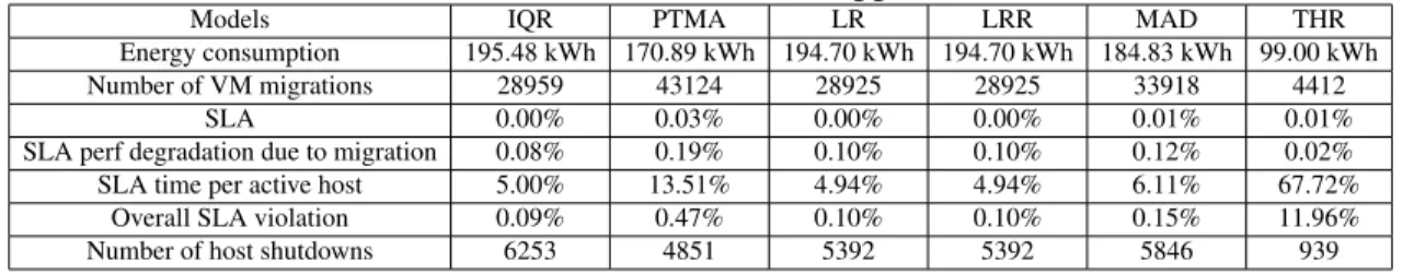
From the Figure 4, we can see that the energy consumption of PTMA is less than the other algorithms. But the number of VM migration is more than others. The overall SLA violation comes to0.47%and SLA active per host is13.51%

Table 6: Planetlab data result for upper threshold

Models IQR PTMA LR LRR MAD THR Energy consumption 195.48 kWh 170.89 kWh 194.70 kWh 194.70 kWh 184.83 kWh 99.00 kWh Number of VM migrations 28959 43124 28925 28925 33918 4412

SLA 0.00% 0.03% 0.00% 0.00% 0.01% 0.01% SLA perf degradation due to migration 0.08% 0.19% 0.10% 0.10% 0.12% 0.02% SLA time per active host 5.00% 13.51% 4.94% 4.94% 6.11% 67.72%

Overall SLA violation 0.09% 0.47% 0.10% 0.10% 0.15% 11.96% Number of host shutdowns 6253 4851 5392 5392 5846 939

6.2.1.2 Result for Selecting Suitableα

Next we run our proposed host upper and host lower algorithm to get the sutable value forα. We run the experiment in the increasing order of 0.5 as shown in the Figure 5 and plot our two sided graphs, considering one graph for migration and energy consump-tion and other graph for SLA and energy consumpconsump-tion. We get a point which is selected as the optimum value from the Figure 5 the two line curves meets at 3.5 in both graphs. So we select it as suitable value and also from the graph we can notice the curve form a parabola shape getting maximum value at the beginning and going to the least value and then start to increase again.

6.2.1.3 Result for Lower and Upper Threshold Value using Optimum Value

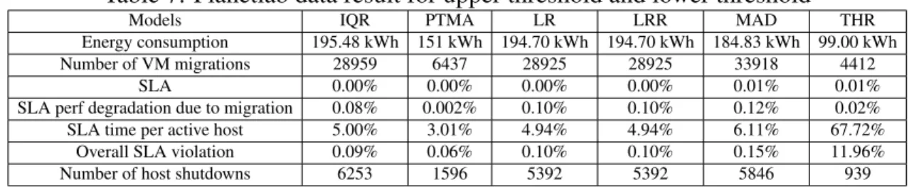
By using our proposed lower and upper algorithm we are able to reduce the en-ergy consumption of data center from170.80to143.21which is shown in Figure 6, This

(45)

(46)

Figure 5: Selecting Optimum Value

Table 7: Planetlab data result for upper threshold and lower threshold Models IQR PTMA LR LRR MAD THR Energy consumption 195.48 kWh 151 kWh 194.70 kWh 194.70 kWh 184.83 kWh 99.00 kWh Number of VM migrations 28959 6437 28925 28925 33918 4412

reduction of power is beneficial to the infrastructure providers as it cuts down the cost. When we compare the number of VM migration, it has been reduced from43124to6431 migrations. This reduction is significant and makes way for bandwidth availability. While SLA is reduced . Host shutdown also reduced by almost70%. Note that THR algorithm consumes less energy, less migration there is a huge difference in the SLA violation as it increase the cost of the service provider.

6.2.2 Result and Analysis of UMKC data

The similar type of comparison as in Section 6.2.1 was followed with the UMKC data.

(47)

(48)

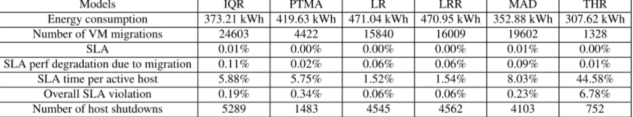
From the Figure 7, our proposed model energy consumption is 344.8kw which is lesser than all the other models. And also, the number of VM migration is reduced to 15616 where as the other models have higher number of migrations. SLA seems to be higher than other three models LRR, MAD and THR and also the number of host shutdown is less.

Table 8: UMKC data result for upper threshold

Models IQR PTMA LR LRR MAD THR Energy consumption 373.21 kWh 344.80 kWh 471.04 kWh 470.95 kWh 352.88 kWh 307.62 kWh Number of VM migrations 24603 15616 15840 16009 19602 1328

6.2.2.2 Result for Selecting Suitableα

From the Figure 8 we can see that the curve for Energy consumption and number of VM migration the curve meets at approximately2.5value αand the graph for energy consumption and Overall SLA violation is found to meet at approximately3. Since theα

is favouring the energy consumption, we selectαvalue as2.5.

6.2.2.3 Result for Lower and Upper Threshold Value Using Optimum Value

Since we have selected α as 2.5, surprisingly our lower threshold energy con-sumption has increased from 344.8 to 419.63 from the Figure 9 this is due to decrease in the host shutdown. The SLA performance degradation due to migration has decreased from0.08% to0.02%. This is due to the number of migration decreasing from15616to

(49)

(50)

4422. Using lower threshold, we were able to minimize the VM migration and SLA but not Enegry. If we need to minimize Energy consumption, then we have to chooseαless than2.5.

Table 9: UMKC data result for upper threshold and lower threshold Models IQR PTMA LR LRR MAD THR Energy consumption 373.21 kWh 419.63 kWh 471.04 kWh 470.95 kWh 352.88 kWh 307.62 kWh Number of VM migrations 24603 4422 15840 16009 19602 1328

6.2.3 Result and Analysis of Google data

The similar type of comparison as in Section 6.2.1 is followed with the Google data trace.

According to the result from the simulation, we can see that the energy consump-tion of our upper threshold is better than the IQR and MAD but there is a slight increase in the power compared to the LR and THR Figure 10 The number of VM migration of

(51)

(52)

our PTMA is at1418compared to the LR and lRR algortihm which has1408migrations, a small increase in migrations. Next comes the SLA. From the figure, we can make out that our algorithm is not better than the other algorithms. Number of VM migration is observed to be reduced compared to the other algorithms.

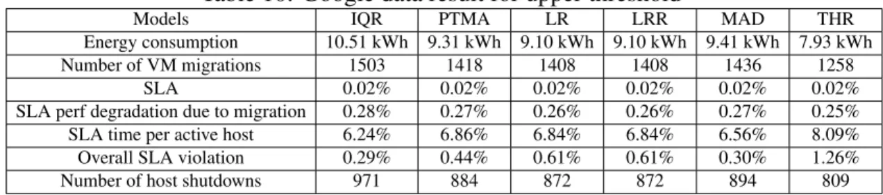
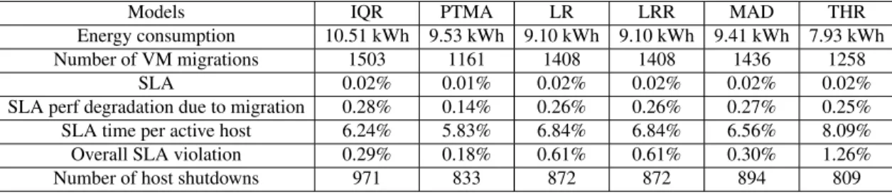
Table 10: Google data result for upper threshold

Models IQR PTMA LR LRR MAD THR

Energy consumption 10.51 kWh 9.31 kWh 9.10 kWh 9.10 kWh 9.41 kWh 7.93 kWh

Number of VM migrations 1503 1418 1408 1408 1436 1258

SLA 0.02% 0.02% 0.02% 0.02% 0.02% 0.02%

SLA perf degradation due to migration 0.28% 0.27% 0.26% 0.26% 0.27% 0.25%

SLA time per active host 6.24% 6.86% 6.84% 6.84% 6.56% 8.09%

Overall SLA violation 0.29% 0.44% 0.61% 0.61% 0.30% 1.26%

Number of host shutdowns 971 884 872 872 894 809

6.2.3.2 Result for Selecting Optimum Value

We have plotted the Enegry vs SLA violation and Energy vs VM’s migration and found that the curve meets around 2.5 Figure 11. so we select theαas 2.5.

6.2.3.3 Result for Lower and Upper Threshold Value Using Optimum Value

From the Figure 12 we can find that except for the enegry consumption, there is a decrease in the SLA,VM migration, and the number of host shutdown. The migration is low compared to other algorithms at 1161. that can increase the residual bandwidth availability. The SLA performance due to migration has been reduced from 0.27% to 0.14%compared to the upper threshold algorithm. As the number of host shutdown has decreased, the power consumption increases. Even though it has failed to increase the number of host shutdown, SLA time per host has been reduced by6.8%to5.8%. Overall there is a slight increase in the enegry but BW and SLA has considerably decreased.

(53)

(54)

Table 11: Google data result for upper threshold and lower threshold

Models IQR PTMA LR LRR MAD THR

Energy consumption 10.51 kWh 9.53 kWh 9.10 kWh 9.10 kWh 9.41 kWh 7.93 kWh

Number of VM migrations 1503 1161 1408 1408 1436 1258

SLA 0.02% 0.01% 0.02% 0.02% 0.02% 0.02%

SLA perf degradation due to migration 0.28% 0.14% 0.26% 0.26% 0.27% 0.25%

SLA time per active host 6.24% 5.83% 6.84% 6.84% 6.56% 8.09%

Overall SLA violation 0.29% 0.18% 0.61% 0.61% 0.30% 1.26%

(55)

(56)

CHAPTER 7 CONCLUSION

In our thesis we proposed a new model to balance the energy and the performance of a datacenter by implementing an adaptive host upper utilization threshold and a host lower utilization threshold for CPU utilization in a host. The simulation result shows that our proposed algorithm consumes less power, bandwidth with minimal SLA viola-tion as compared to the existing algorithms. We applied our algorithm to compare the datacenter’s data traces of Planetlab, UMKC and Google. We found out that in planetlab, energy consumption and SLA violation can be reduced and the residual bandwidth can be increased. In UMKC data with upper threshold energy consumption is less where as in lower and upper threshold energy consumption increases slightly but SLA violation decreases and residual BW increases. In case of Google data, the SLA violations and the residual BW decreases with a slight increase in power consumption.

In future Simulation can be extended to migrate VM between datacenters and an algorithm can be developed to find theα. Every new model has its own drawbacks. In our algorithm there is no cost specified for the SLA violations and power consumption, which makes it difficult to compare power and SLA as a parameter. Simulation need to be done for various value ofα to find the suitable value, which is a time consuming process. Except for the UMKC data, the two data available are too old to come to a better conclusion.

(57)

APPENDIX A INFORMATION A.1 Workload Pattern

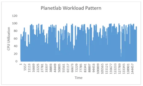
The data from datacenters have been plotted to study the workload pattern. As you can see from the Figure 13 the planet lab data has CPU utilization100% most of the time.

Figure 13: Panetlab Workload Pattern

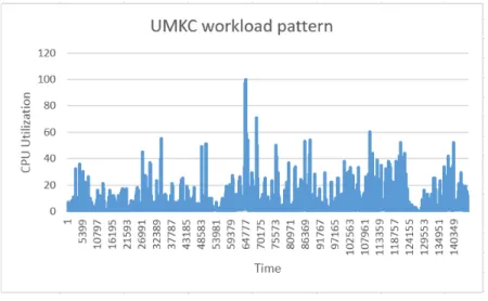
From the Figure 14 UMKC datacenter has reached 100% utilization only few times. most of the times it reaches up to60% utilization but most of the times remains under 40%. The UMKC datacenter from the workload pattern we can say that its been less utilized.

(58)

Figure 14: UMKC Workload Pattern

Since the data has been obfuscated we cant come to clear conclusion about the workload pattern of google datacenter.

(59)

A.2 Number of VM migration

A analysis of pattern of VM migrations for all the models which are available inside Cloudsim and our proposed model have been shown in this section. We consider the VM which has highest migration compared to other VM’s.

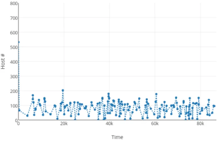
A.2.1 For Planetlab

For IQR model we have found VM792has highest number of migration. From the Figure 16 Initially the placement of VM takes place in ascending order of Host number. During its lifetime we can see from the Figure that VM migrates between 0th host and 200thhost. This can be observed with other models except PTMA model which is shown in Figure 17. In PTMA model the VM migrates up to host number 610 and the VM migration is random from what we see from the figures.

We have compared the VM 1012 of PTMA model with VM 1012 of all other models and found out to be that the VM is concentrated over time between0thand200th

host.

A.2.2 For UMKC

For UMKC data we see that form the Figure 23 for IQR model the highest number of VM migrations is for VM488 and found to be concentrated between 0th and 100th

over time and it same for all other models except for PTMA model which has reached up to450thhost.

(60)

Figure 16: Planetlab VM migration for VM 792 IQR model

(61)

Figure 18: Planetlab VM migration for VM 844 LR model

(62)

Figure 20: Planetlab VM migration for VM 987 MAD model

(63)

Figure 22: Planetlab VM migration for VM 1012 for all the models

50thhost over a time when we consider the VM308which happens to be the worst VM for our proposed model from the Figure 29

A.2.3 For Google

When we consider google data for IQR model, from the Figure 30 VM 942 has highest number of VM migration. It has almost exponentially decreasing curve in all of the models. when we consider the VM 218 which happens to be highest in-case of our proposed model which is shown in Figure 36 we can see same behaviour that is exponentially decreasing over time.

(64)

Figure 23: UMKC VM migration for VM 488 IQR model

(65)

Figure 25: UMKC VM migration for VM 399 LR model

(66)

Figure 27: UMKC VM migration for VM 453 MAD model

(67)

Figure 29: UMKC VM migration for VM 308 for all the models

(68)

Figure 31: Google VM migration for VM 218 PTMA model

(69)

Figure 33: Google VM migration for VM 943 LRR model

(70)

Figure 35: Google VM migration for VM 265 THR model

(71)

A.3 Frequency of VM migration

We did analysis on Vm migration for three different datasets considering all the models. From the Figure 37, our proposed model has the highest number of migration of a single VM to be68and the VM’s which has less number of VM migration to be more for Planetlab datasets from this we can infer that there is less VM migrations.

Figure 37: VM migrations for Planetlab data

when we consider the UMKC datasets for VM migration, from the Figure 38 we can see that maximum number of times the VM migration happens to be14for our proposed model where as for other models its exceeds14and occurrence of VM migration for least number of times VM migration found to be more.

From the Figure 39, even though the graphs looks similar but when you have a close look at it, occurrence of VM migration found to be the highest for least number of times VM migration and the maximum number of a time the single VM migrates found to be8.

(72)

Figure 38: VM migrations for UMKC data

(73)

REFERENCE LIST

[1] VMware Distributed Power Management: Concepts

and Usage. https://www.vmware.com/techpapers/2008/

vmware-distributed-power-management-concepts-and-1080.html.

[2] Armbrust, M., Fox, A., Griffith, R., Joseph, A. D., Katz, R., Konwinski, A., Lee, G., Patterson, D., Rabkin, A., Stoica, I., et al. A view of cloud computing. Communi-cations of the ACM 53, 4 (2010), 50–58.

[3] Beloglazov, A., and Buyya, R. Optimal online deterministic algorithms and adap-tive heuristics for energy and performance efficient dynamic consolidation of virtual machines in cloud data centers.Concurrency and Computation: Practice and Expe-rience 24, 13 (2012), 1397–1420.

[4] Bobroff, N., Kochut, A., and Beaty, K. Dynamic placement of virtual machines for managing sla violations. In Proc. of 2007 10th IFIP/IEEE International Symposium on Integrated Network Management(2007), IEEE, pp. 119–128.

[5] Boutaba, R., Zhang, Q., and Zhani, M. F. Virtual machine migration in cloud com-puting environments: Benefits, challenges, and approaches. InCommunication In-frastructures for Cloud Computing, H. Mouftah and B. Kantarci, Eds. IGI-Global, USA, 2013, pp. 383–408.

(74)

[6] Calheiros, R. N., Ranjan, R., Beloglazov, A., De Rose, C. A., and Buyya, R. CloudSim: a toolkit for modeling and simulation of cloud computing environments and evaluation of resource provisioning algorithms.Software: Practice and Experi-ence 41, 1 (2011), 23–50.

[7] Chhibber, A., and Batra, S. Security analysis of cloud computing. International Journal of Advanced Research in Engineering and Applied Sciences 2, 3 (2013), 2278–6252.

[8] Cleveland, W. S. Robust locally weighted regression and smoothing scatterplots.

Journal of the American Statistical Association 74, 368 (1979), 829–836. [9] Cleveland, W. S. Visualizing Data. Hobart Press, 1993.

[10] Cleveland, W. S., and Loader, C. Smoothing by local regression: Principles and methods. InStatistical theory and computational aspects of smoothing. Springer, 1996, pp. 10–49.

[11] Fan, X., Weber, W.-D., and Barroso, L. A. Power provisioning for a warehouse-sized computer. ACM SIGARCH Computer Architecture News 35, 2 (2007), 13–23. [12] Farahnakian, F., Pahikkala, T., Liljeberg, P., and Plosila, J. Energy aware

consoli-dation algorithm based on K-nearest neighbor regression for cloud data centers. In

Utility and Cloud Computing (UCC), 2013 IEEE/ACM 6th International Conference on(2013), IEEE, pp. 256–259.

(75)

[13] Goiri, Í., Julià, F., Fitó, J. O., Mac´ıas, M., and Guitart, J. Resource-level QoS metric for CPU-based guarantees in Cloud providers. In International Workshop on Grid Economics and Business Models(2010), Springer, pp. 34–47.

[14] Maltais, M. Who owns your stuff in the cloud? Los Angeles Times(April 26,2012). [15] Maurya, K., and Sinha, R. Energy conscious dynamic provisioning of virtual ma-chines using adaptive migration thresholds in cloud data center. International Jour-nal of Computer Science and Mobile Computing 2, 3 (2013), 74–82.

[16] Mell, P., and Grance, T. The NIST definition of cloud computing. Communications of the ACM 53, 6 (2010), 50.

[17] Metkar, G., Agrawal, S., and Singh, D. S. A live migration of virtual machine based on the dynamic threshold at cloud data centres. International Journal of Advanced Research in Computer Science and Software Engineering 3, 10 (2013), 401–405. [18] Minas, L., and Ellison, B. Energy efficiency for information technology: How to

reduce power consumption in servers and data centers. Intel Press, 2009.

[19] Nathuji, R., and Schwan, K. VirtualPower: Coordinated power management in vir-tualized enterprise systems. ACM SIGOPS Operating Systems Review 41, 6 (2007), 265–278.

[20] Park, K., and Pai, V. S. CoMon: a mostly-scalable monitoring system for PlanetLab.

(76)

[21] Prodan, R., and Ostermann, S. A survey and taxonomy of infrastructure as a service and web hosting cloud providers. In Proc. of 2009 10th IEEE/ACM International Conference on Grid Computing(2009), IEEE, pp. 17–25.

[22] Reiss, C., Wilkes, J., and Hellerstein, J. L. Google cluster-usage traces: For-mat + schema. Technical report, Google Inc., Mountain View, CA, USA, Nov. 2011. Revised 2012.03.20. Posted at http://code.google.com/p/googleclusterdata/ wiki/TraceVersion2.

[23] Reiss, C., Wilkes, J., and Hellerstein, J. L. Obfuscatory obscanturism: making workload traces of commercially-sensitive systems safe to release. In Proc. of 3rd International Workshop on Cloud Management (CLOUDMAN) (Maui, HI, USA, Apr. 2012), IEEE, pp. 1279–1286.

[24] Rimal, B. P., Choi, E., and Lumb, I. A taxonomy and survey of cloud computing systems. INC, IMS and IDC(2009), 44–51.

[25] Ryan, M. Cloud computing privacy concerns on our doorstep. Communications of the ACM 54, 1 (2011), 36–38.

[26] Takeda, S., and Takemura, T. A rank-based vm consolidation method for power saving in datacenters. Information and Media Technologies 5, 3 (2010), 994–1002.

(77)

VITA

Amarnath Beedimane Hanumantharaya was born on February 13, 1991 in Ban-galore, Karnataka, India. He was educated in local public schools and graduated from Visveswaraya Technological University in 2012 with B.E. degree in Electronics and Com-munication.