Massachusetts Institute of Technology
Department of Economics
Working Paper Series
LEAST SQUARES AFTER MODEL SELECTION IN
HIGH-DIMENSIONAL SPARSE MODELS
Alexandre Belloni
Victor Chernozhukov
Working Paper 10-5
January 4, 2009
Revised: June 14, 2011
Room E52-251
50 Memorial Drive
Cambridge, MA 02142
This paper can be downloaded without charge from the
Social Science Research Network Paper Collection at
arXiv:1001.0188v3 [math.ST] 11 Jun 2011
HIGH-DIMENSIONAL SPARSE MODELS
ALEXANDRE BELLONI AND VICTOR CHERNOZHUKOV
Abstract. In this paper we study post-model selection estimators which ap-ply ordinary least squares (ols) to the model selected by first-step penalized estimators, typically lasso. It is well known that lasso can estimate the non-parametric regression function at nearly the oracle rate, and is thus hard to improve upon. We show that ols post lasso estimator performs at least as well as lasso in terms of the rate of convergence, and has the advantage of a smaller bias. Remarkably, this performance occurs even if the lasso-based model selection “fails” in the sense of missing some components of the “true” regression model. By the “true” model we mean here the bests-dimensional approximation to the nonparametric regression function chosen by the oracle. Furthermore, ols post lasso estimator can perform strictly better than lasso, in the sense of a strictly faster rate of convergence, if the lasso-based model selec-tion correctly includes all components of the “true” model as a subset and also achieves sufficient sparsity. In the extreme case, when lasso perfectly selects the “true” model, the ols post lasso estimator becomes the oracle estimator. An important ingredient in our analysis is a new sparsity bound on the dimen-sion of the model selected by lasso which guarantees that this dimendimen-sion is at most of the same order as the dimension of the “true” model. Our rate results are non-asymptotic and hold in both parametric and nonparametric models. Moreover, our analysis is not limited to the lasso estimator acting as selector in the first step, but also applies to any other estimator, for example various forms of thresholded lasso, with good rates and good sparsity properties. Our analysis covers both traditional thresholding and a new practical, data-driven thresholding scheme that induces maximal sparsity subject to maintaining a certain goodness-of-fit. The latter scheme has theoretical guarantees similar to those of lasso or ols post lasso, but it dominates these procedures as well as traditional thresholding in a wide variety of experiments.
First arXiv version: December 2009.
Key words. lasso, ols post lasso, post-model-selection estimators. AMS Codes. Primary 62H12, 62J99; secondary 62J07.
1. Introduction
In this work we study post-model selected estimators for linear regression in high-dimensional sparse models (hdsms). In such models, the overall number of
regressorspis very large, possibly much larger than the sample size n. However,
there ares=o(n) regressors that capture most of the impact of all covariates on
the response variable. hdsms ([9], [22]) have emerged to deal with many new
ap-plications arising in biometrics, signal processing, machine learning, econometrics,
Date: First Version: January 4, 2009. Current Revision: June 14, 2011. Former title:“Post-ℓ1
-Penalized Estimators in High-dimensional Linear Regression Models.”.
and other areas of data analysis where high-dimensional data sets have become widely available.
Several papers have begun to investigate estimation of hdsms, primarily
focus-ing on mean regression with the ℓ1-norm acting as a penalty function [4, 6, 7,
8, 9, 17, 22, 28, 31, 33]. The results in [4, 6, 7, 8, 17, 22, 31, 33] demonstrated
the fundamental result that ℓ1-penalized least squares estimators achieve the rate
p
s/n√logp, which is very close to the oracle rateps/nachievable when the true
model is known. The works [17, 28] demonstrated a similar fundamental result
on the excess forecasting error loss under both quadratic and non-quadratic loss functions. Thus the estimator can be consistent and can have excellent forecasting performance even under very rapid, nearly exponential growth of the total number
of regressorsp. Also, [2] investigated the ℓ1-penalized quantile regression process,
obtaining similar results. See [4,6, 7, 8, 15,19,20, 24] for many other interesting
developments and a detailed review of the existing literature.
In this paper we derive theoretical properties of post-model selection estimators which apply ordinary least squares (ols) to the model selected by first-step penal-ized estimators, typically lasso. It is well known that lasso can estimate the mean regression function at nearly the oracle rate, and hence is hard to improve upon. We show that ols post lasso can perform at least as well as lasso in terms of the rate of convergence, and has the advantage of a smaller bias. This nice performance occurs even if the lasso-based model selection “fails” in the sense of missing some components of the “true” regression model. Here by the “true” model we mean the
bests-dimensional approximation to the regression function chosen by the oracle.
The intuition for this result is that lasso-based model selection omits only those components with relatively small coefficients. Furthermore, ols post lasso can per-form strictly better than lasso, in the sense of a strictly faster rate of convergence, if the lasso-based model correctly includes all components of the “true” model as a subset and is sufficiently sparse. Of course, in the extreme case, when lasso perfectly selects the “true” model, the ols post lasso estimator becomes the oracle estimator. Importantly, our rate analysis is not limited to the lasso estimator in the first step, but applies to a wide variety of other first-step estimators, including, for example, thresholded lasso, the Dantzig selector, and their various modifications. We give generic rate results that cover any first-step estimator for which a rate and a sparsity bound are available. We also give a generic result on using thresholded lasso as the first-step estimator, where thresholding can be performed by a traditional thresholding scheme (t-lasso) or by a new fitness-thresholding scheme we introduce in the paper (fit-lasso). The new thresholding scheme induces maximal sparsity subject to maintaining a certain goodness-of-fit in the sample, and is completely data-driven. We show that ols post fit-lasso estimator performs at least as well as the lasso estimator, but can be strictly better under good model selection properties. Finally, we conduct a series of computational experiments and find that the
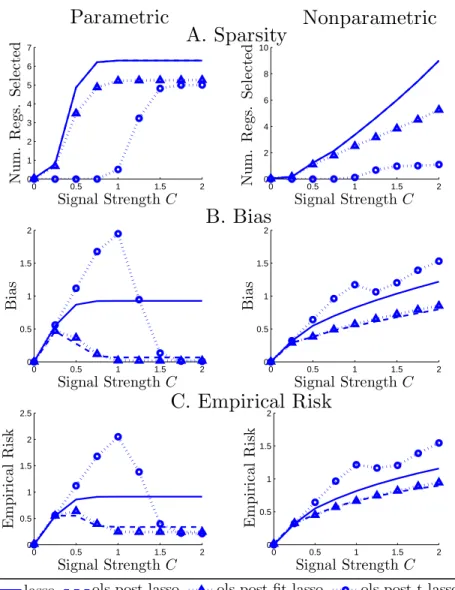
results confirm our theoretical findings. Figure 1 is a brief graphical summary of
our theoretical results showing how the empirical risk of various estimators change
with the signal strengthC(coefficients of relevant covariates are set equal toC). For
very low level of signal, all estimators perform similarly. When the signal strength is intermediate, ols post lasso and ols post fit-lasso substantially outperform lasso and the ols post t-lasso estimators. However, we find that the ols post fit-lasso outperforms ols post lasso whenever lasso does not produce very sparse solutions
which occurs if the signal strength level is not low. For large levels of signal, ols post fit-lasso and ols post t-lasso perform very well improving upon lasso and ols post lasso. Thus, the main message here is that ols post lasso and ols post fit-lasso perform at least as well as lasso and sometimes a lot better.
0 0.5 1 1.5 2 2.5 3 0 0.5 1 1.5 2 2.5
E
mp
ir
ic
al
R
is
k
Signal Strength
C
Empirical Risk
lasso ols post lasso ols post fit-lasso ols post t-lassoFigure 1. This figure plots the performance of the estimators listed in the text under the equi-correlated design for the covariates xi ∼ N(0,Σ),
Σjk= 1/2 ifj6=k. The number of regressors isp= 500 and the sample size
isn= 100 with 1000 simulations for each level of signal strengthC. In each simulation there are 5 relevant covariates whose coefficients are set equal to the signal strengthC, and the variance of the noise is set to 1.
To the best of our knowledge, our paper is the first to establish the aforemen-tioned rate results on ols post lasso and the proposed ols post fitness-thresholded
lasso in the mean regression problem. Our analysis builds upon the ideas in [2],
who established the properties of post-penalized procedures for the related, but dif-ferent, problem of median regression. Our analysis also builds on the fundamental
results of [4] and the other works cited above that established the properties of the
first-step lasso-type estimators. An important ingredient in our analysis is a new sparsity bound on the dimension of the model selected by lasso, which guarantees that this dimension is at most of the same order as the dimension of the “true” model. This result builds on some inequalities for sparse eigenvalues and reasoning
previously given in [2] in the context of median regression. Our sparsity bounds for
lasso improve upon the analogous bounds in [4] and are comparable to the bounds
in [33] obtained under a larger penalty level. We also rely on maximal inequalities
in [33] to provide primitive conditions for the sharp sparsity bounds to hold.
We organize the paper as follows. Section 2 reviews the model and discusses the
estimators. Section 3 revisits some benchmark results of [4] for lasso, albeit allowing
for a data driven choice of penalty level, develops an extension of model selection
results of [19] to the nonparametric case, and derives a new sparsity bound for
lasso. Section 4 presents a generic rate result on ols post-model selection estimators. Section 5 applies the generic results to the ols post lasso and the ols post thresholded lasso estimators. Appendix contains main proofs and the Supplementary Appendix
contains auxiliary proofs. In the Supplementary Appendix we also present the results of our computational experiments.
Notation. In making asymptotic statements, we assume that n → ∞ and
p=pn → ∞, and we also allow fors =sn → ∞. In what follows, all parameter
values are indexed by the sample sizen, but we omit the index whenever this does
not cause confusion. We use the notation (a)+ = max{a,0}, a∨b = max{a, b}
anda∧b= min{a, b}. Theℓ2-norm is denoted byk · k, the ℓ1-norm is denoted by
k · k1, theℓ∞-norm is denoted byk · k∞, and theℓ0-normk · k0denotes the number
of non-zero components of a vector. Given a vector δ∈ IRp, and a set of indices
T ⊂ {1, . . . , p}, we denote by δT the vector in which δT j = δj if j ∈ T, δT j = 0
if j /∈T, and by |T| the cardinality ofT. Given a covariate vector xi ∈ IRp, we
denote byxi[T] vector{xij, j∈T}. The symbolE[·] denotes the expectation. We
also use standard empirical process notation
En[f(z•)] := n X i=1 f(zi)/n and Gn(f(z•)) := n X i=1 (f(zi)−E[f(zi)])/√n.
We also denote the L2(P
n)-norm by kfkPn,2 = (En[f
2
•])1/2. Given covariate
val-ues x1, . . . , xn, we define the prediction norm of a vector δ ∈ IRp as kδk2,n = {En[(x′
iδ)2]}1/2. We use the notation a. b to denote a ≤Cb for some constant
C > 0 that does not depend on n (and therefore does not depend on quantities
indexed bynlikepors); anda.P b to denotea=OP(b). For an eventA, we say
thatA wp→1 whenAoccurs with probability approaching one asngrows. Also
we denote by ¯c= (c+ 1)/(c−1) for a chosen constantc >1.
2. The setting, estimators, and conditions 2.1. The setting.
Condition( M ). We have data {(yi, zi), i= 1, . . . , n} such that for eachn
yi=f(zi) +ǫi, ǫi∼N(0, σ2), i= 1, ..., n, (2.1)
whereyiare the outcomes,ziare vectors of fixed regressors, andǫi are i.i.d. errors.
Let P(zi) be a given p-dimensional dictionary of technical regressors with respect
zi, i.e. a p-vector of transformation of zi, with components
xi:=P(zi)
of the dictionary normalized so that
En[x2
•j] = 1for j = 1, . . . , p.
In making making asymptotic statements, we assume thatn→ ∞andp=pn→ ∞,
and that all parameters of the model are implicitly indexed by n.
We would like to estimate the nonparametric regression functionf at the design
points, namely the valuesfi=f(zi) fori= 1, ..., n. In order to setup estimation and
define a performance benchmark we consider the following oracle risk minimization program: min 0≤k≤p∧nc 2 k+σ2 k n, (2.2) where c2k:= min kβk0≤k En[(f•−x′ •β)2]. (2.3)
Note that c2
k +σ2k/n is an upper bound on the risk of the best k-sparse least
squares estimator, i.e. the best estimator amongst all least squares estimators that
usekout ofpcomponents ofxi to estimatefi, fori= 1, ..., n. The oracle program
(2.2) chooses the optimal value of k. Let sbe the smallest integer amongst these
optimal values, and let
β0∈arg min
kβk0≤s
En[(f•−x′
•β)2]. (2.4)
We callβ0 the oracle target value,T := support(β0) the oracle model,s:=|T|=
kβ0k0 the dimension of the oracle model, andx′iβ0 the oracle approximation tofi.
The latter is our intermediary target, which is equal to the ultimate targetfi up
to the approximation error
ri:=fi−x′iβ0.
If we knewTwe could simply usexi[T] as regressors and estimatefi, fori= 1, ..., n,
using the least squares estimator, achieving the risk of at most
c2s+σ2s/n,
which we call the oracle risk. Since T is not known, we shall estimate T using
lasso-type methods and analyze the properties of post-model selection least squares estimators, accounting for possible model selection mistakes.
Remark 2.1 (The oracle program). Note that if argmin is not unique in the problem
(2.4), it suffices to select one of the values in the set of argmins. Supplementary
Appendix provides a more detailed discussion of the oracle problem. The idea of
using oracle problems such as (2.2) for benchmarking the performance follows its
prior uses in the literature. For instance, see [4], Theorem 6.1, where an analogous
problem appears in upper bounds on performance of lasso.
Remark 2.2 (A leading special case). When contrasting the performance of lasso and ols post lasso estimators in Remarks 5.1-5.2 given later, we shall mention a balanced case where
c2s.σ2s/n (2.5)
which says that the oracle program (2.2) is able to balance the norm of the bias
squared to be not much larger than the variance term σ2s/n. This corresponds
to the case that the approximation error bias does not dominate the estimation error of the oracle least squares estimator, so that the oracle rate of convergence
simplifies tops/nmentioned in the introduction.
2.2. Model selectors based on lasso. Given the large number of regressors
p > n, some regularization or covariate selection is required in order to obtain
consistency. The lasso estimator [26], defined as follows, achieves both tasks by
using theℓ1 penalization:
b β∈arg min β∈RpQb(β) + λ nkβk1, where Qb(β) =En[(y•−x ′ •β)2], (2.6)
and λ is the penalty level whose choice is described below. If the solution is not
unique we pick any solution with minimum support. The lasso is often used as an estimator and more often only as a model selection device, with the model selected by lasso given by:
b
Moreover, we denote bymb :=|Tb\T|the number of components outsideT selected
by lasso and byfbi=x′iβ, ib = 1, ..., nthe lasso estimate of fi, i= 1, ..., n.
Oftentimes additional thresholding is applied to remove regressors with small estimated coefficients, defining the so called thresholded lasso estimator:
b
β(t) = (βbj1{|βbj|> t}, j= 1, ..., p), (2.7)
wheret≥0 is the thresholding level, and the corresponding selected model is then
b
T(t) := support(βb(t)).
Note that settingt= 0, we haveTb(t) =Tb, so lasso is a special case of thresholded
lasso.
2.3. Post-model selection estimators. Given this all of our post-model selection estimators or ols post lasso estimators will take the form
e
βt= arg min
β∈IRpQb(β) :βj= 0 for eachj∈Tb
c(t). (2.8)
That is given the model selected a threshold lassoTb(t), including the lasso’s model
b
T(0) as a special case, the post-model selection estimator applies the ordinary least
squares to the selected model.
In addition to the case oft = 0, we also consider the following choices for the
threshold level:
traditional threshold (t): t > ζ= max
1≤j≤p|βbj−β0j|,
fitness-based threshold (fit): t=tγ := max
t≥0{t:Qb(βe
t)−Qb(βb)≤γ}, (2.9)
whereγ≤0, and|γ|is the gain of the in-sample fit allowed relative to lasso.
As discussed in Section 3.2, the standard thresholding method is particularly
appealing in models in which oracle coefficients β0 are well separated from zero.
This scheme however may perform poorly in models with oracle coefficients not well separated from zero and in nonparametric models. Indeed, even in parametric models with many small but non-zero true coefficients, thresholding the estimates too aggressively may result in large goodness-of-fit losses, and consequently in slow rates of convergence and even inconsistency for the second-step estimators. This issue directly motivates our new goodness-of-fit based thresholding method, which sets to zero small coefficient estimates as much as possible subject to maintaining a certain goodness-of-fit level.
Depending on how we select the threshold, we consider the following three types of the post-model selection estimators:
ols post lasso: βe0 (t= 0),
ols post t-lasso: βet (t > ζ),
ols post fit-lasso: βetγ (t=t
γ).
(2.10) The first estimator is defined by ols applied to the model selected by lasso, also called Gauss-lasso; the second by ols applied to the model selected by the thresholded lasso, and the third by ols applied to the model selected by fitness-thresholded lasso.
The main purpose of this paper is to derive the properties of the post-model
selection estimators (2.10). If model selection works perfectly, which is possible
are the oracle estimators, whose properties are well known. However, of a much more general interest is the case when model selection does not work perfectly, as occurs for many designs of interest in applications.
2.4. Choice and computation of penalty level for lasso. The key quantity in
the analysis is the gradient ofQb at the true value:
S= 2En[x•ǫ•].
This gradient is the effective “noise” in the problem that should be dominated by the regularization. However we would like to make the bias as small as possible.
This reasoning suggests choosing the smallest penalty levelλso that to dominate
the noise, namely
λ≥cnkSk∞ with probability at least 1−α, (2.11)
where probability 1−αneeds to be close to 1 and c > 1. Therefore, we propose
setting
λ=c′ σbΛ(1−α|X),for some fixed c′> c >1, (2.12)
where Λ(1−α|X) is the (1−α)-quantile of nkS/σk∞, andbσ is a possibly
data-driven estimate of σ. Note that the quantity Λ(1−α|X) is independent ofσ and
can be easily approximated by simulation. We refer to this choice of λ as the
data-driven choice, reflecting the dependence of the choice on the design matrix
X = [x1, . . . , xn]′ and a possibly data-driven bσ. Note that the proposed (2.12) is
sharper than c′bσ2p2nlog(p/α) typically used in the literature. We impose the
following conditions onσb.
Condition(V). The estimatedσb obeys
ℓ≤bσ/σ≤uwith probability at least1−τ,
where0< ℓ≤1 and1≤uand0≤τ <1 be constants possibly dependent onn.
We can construct a σb that satisfies this condition under mild assumptions as
follows. First, set bσ = bσ0, where σb0 is an upper bound on σ which is possibly
data-driven, for example the sample standard deviation ofyi. Second, compute the
lasso estimator based on this estimate and setbσ2=Qb(βb). We demonstrate thatbσ
constructed in this way satisfies Condition V and characterize quantities uand ℓ
andτ in the Supplementary Appendix. We can iterate on the last step a bounded
number of times. Moreover, we can similarly use ols post lasso for this purpose. 2.5. Choices and computation of thresholding levels. Our analysis will cover a wide range of possible threshold levels. Here, however, we would like to propose some basic options that give both good finite-sample and theoretical results. In the traditional thresholding method, we can set
t= ˜cλ/n, (2.13)
for some ˜c≥1. This choice is theoretically motivated by Section 3.2 that presents
the perfect model selection results, where under some conditions ζ ≤˜cλ/n. This
choice also leads to near-oracle performance of the resulting post-model selection
estimator. Regarding the choice of ˜c, we note that setting ˜c= 1 and achievingζ≤
λ/nis possible by the results of Section 3.2 if empirical Gram matrix is orthogonal
thresholding one can perform under conditions of Section 3.2 (note also that ˜c= 1
has performed better than ˜c >1 in our computational experiments).
Our fitness-based thresholdtγ requires the specification of the parameterγ. The
simplest choice delivering near-oracle performance isγ= 0; this choice leads to the
sparsest post-model selection estimator that has the same in-sample fit as lasso. Our preferred choice is however to set
γ=Qb(βe
0)−Qb(βb)
2 <0, (2.14)
whereβe0is the ols post lasso estimator. The resulting estimator is more sparse than
lasso, and it also produces a better in-sample fit than lasso. This choice also results in near-oracle performance and also leads to the best performance in computational
experiments. Note also that for anyγ, we can computetγ by a binary search over
t∈sort{|βbj|, j∈Tb}, where sort is the sorting operator. This is the case since the
final estimator depends only on the selected support and not on the specific value
oft used. Therefore, since there are at most|Tb| different values oftto be tested,
by using a binary search, we can computetγ exactly by running at most⌈log2|Tb|⌉
ordinary least squares problems.
2.6. Conditions on the design. For the analysis of lasso we rely on the following restricted eigenvalue condition.
Condition(RE(¯c)). For a given ¯c≥0,
κ(¯c) := min kδT ck1≤¯ckδTk1,δ6=0 √s kδk2,n kδTk1 >0.
This condition is a variant of the restricted eigenvalue condition introduced in [4],
that is known to be quite general and plausible; see also [4] for related conditions.
For the analysis of post-model selection estimators we need the following re-stricted sparse eigenvalue condition.
Condition(RSE(m)). For a given m < n,
e κ(m)2:= min kδT ck0≤m,δ6=0 kδk2 2,n kδk2 >0, φ(m) :=kδ max T ck0≤m,δ6=0 kδk2 2,n kδk2 >0.
Here m denotes the restriction on the number of non-zero components outside
the support T. It will be convenient to define the following condition number
associated with the empirical Gram matrix:
µ(m) =
p
φ(m)
e
κ(m) . (2.15)
The following lemma demonstrates the plausibility of conditions above for the
case where the values xi, i= 1, . . . , n, have been generated as a realization of the
random sample; there are also other primitive conditions. In this case we can expect
that empirical restricted eigenvalue is actually bounded away from zero and (2.15) is
bounded from above with a high probability. The lemma uses the standard concept
of (unrestricted) sparse eigenvalues (see, e.g. [4]) to state a primitive condition on
the population Gram matrix. The lemma allows for standard arbitrary bounded dictionaries, arising in the nonparametric estimation, for example regression splines,
orthogonal polynomials, and trigonometric series, see [14,29,32,27]. Similar results
Lemma 1 (Plausibility of RE and RSE). Suppose x˜i, i = 1, . . . , n, are i.i.d.
zero-mean vectors, such that the population design matrix E[˜xix˜′i] has ones on
the diagonal, and its slogn-sparse eigenvalues are bounded from above by ϕ <
∞ and bounded from below by κ2 > 0. Define x
i as a normalized form of x˜i,
namely xij = ˜xij/(En[˜x2•j])1/2. Suppose that x˜i max1≤i≤nkx˜ik∞ ≤Kn a.s., and
K2
nslog2(n) log2(slogn) log(p∨n) =o(nκ4/ϕ). Then, for anym+s≤slogn, the
empirical restricted sparse eigenvalues obey the following bounds:
φ(m)≤4ϕ, κe(m)2≥κ2/4, and µ(m)≤4√ϕ/κ,
with probability approaching 1 asn→ ∞.
3. Results on lasso as an estimator and model selector The properties of the post-model selection estimators will crucially depend on both the estimation and model selection properties of lasso. In this section we develop the estimation properties of lasso under the data-dependent penalty level,
extending the results of [4], and develop the model selection properties of lasso for
non-parametric models, generalizing the results of [19] to the nonparametric case.
3.1. Estimation Properties of lasso. The following theorem describes the main estimation properties of lasso under the data-driven choice of the penalty level.
Theorem 1 (Performance bounds for lasso under data-driven penalty). Suppose that Conditions M and RE(¯c) hold forc¯= (c+ 1)/(c−1). Ifλ≥cnkSk∞, then
kβb−β0k2,n≤ 1 +1 c λ√s nκ(¯c)+ 2cs.
Moreover, suppose that Condition V holds. Under the data-driven choice (2.12), for c′≥c/ℓ, we have λ≥cnkSk
∞ with probability at least1−α−τ, so that with at least the same probability
kβb−β0k2,n≤(c′+c′/c) √ s nκ(¯c)σuΛ(1−α|X)+2cs, where Λ(1−α|X)≤ p 2nlog(p/α).
If further RE(2¯c) holds, then
kβb−β0k1≤ (1 + 2¯c)√s κ(2¯c) kβb−β0k2,n ∨ 1 + 1 2¯c 2c c−1 n λc 2 s .
This theorem extends the result of [4] by allowing for data-driven penalty level
and deriving the rates in ℓ1-norm. These results may be of independent interest
and are needed for subsequent results.
Remark 3.1. Furthermore, a performance bound for the estimation of the regression function follows from the relation
kfb−fkPn,2− kβb−β0k2,n ≤cs, (3.16)
where fbi =x′iβbis the lasso estimate of the regression function f evaluated at zi.
It is interesting to know some lower bounds on the rate which follow from
Karush-Kuhn-Tucker conditions for lasso (see equation (A.25) in the appendix):
kfb−fkPn,2≥
(1−1/c)λ
q
|Tb|
where mb =|Tb\T|. We note that a similar lower bound was first derived in [21]
withφ(p) instead ofφ(mb).
The preceding theorem and discussion imply the following useful asymptotic bound on the performance of the estimators.
Corollary 1 (Asymptotic bounds on performance of lasso). Under the conditions of Theorem 1, if
φ(mb).1, κ(¯c)&1, µ(mb).1, log(1/α).logp, α=o(1), u/ℓ.1, andτ=o(1)
(3.17)
hold asngrows, we have that
kfb−fkPn,2.P σ
r
slogp n +cs.
Moreover, if |Tb|&P s, in particular ifT ⊆Tb with probability going to1, we have
kfb−fkPn,2&P σ
r
slogp n .
In Lemma1we established fairly general sufficient conditions for the first three
relations in (3.17) to hold with high probability asngrows, when the design points
z1, ..., zn were generated as a random sample. The remaining relations are mild
conditions on the choice ofαand the estimation ofσthat are used in the definition
of the data-driven choice (2.12) of the penalty levelλ.
It follows from the corollary that providedκ(¯c) is bounded away from zero, lasso
with data-driven penalty estimates the regression function at a near-oracle rate. The second part of the corollary generalizes to the nonparametric case the lower
bound obtained for lasso in [21]. It shows that the rate cannot be improved in
gen-eral. We shall use the asymptotic rates of convergence to compare the performance of lasso and the post-model selection estimators.
3.2. Model selection properties of lasso. The main results of the paper do not require the first-step estimators like lasso to perfectly select the “true” oracle model. In fact, we are specifically interested in the most common cases where these estimators do not perfectly select the true model. For these cases, we will prove that post-model selection estimators such as ols post lasso achieve near-oracle rates like those of lasso. However, in some special cases, where perfect model selection is possible, these estimators can achieve the exact oracle rates, and thus can be even better than lasso. The purpose of this section is to describe these very special cases where perfect model selection is possible.
Theorem 2(Some conditions for perfect model selection in nonparametric setting).
Suppose that Condition M holds. (1) If the coefficients are well separated from zero, that is
min
j∈T|β0j|> ζ+t, for somet≥ζ:= maxj=1,...,p|βbj−β0j|,
then the true model is a subset of the selected model, T := support(β0) ⊆ Tb :=
support(βb).Moreover,T can be perfectly selected by applying leveltthresholding to
b
(2) In particular, if λ ≥ cnkSk∞, and there is a constant U > 5¯c such that the empirical Gram matrix satisfies |En[x•jx•k]| ≤1/(U s)for all1≤j < k≤p, then
ζ≤ λn·UU+ ¯c −5¯c+ σ √ n∧cs+ 6¯c U−5¯c cs √ s+ 4¯c U n λ c2 s s.
These results substantively generalize the parametric results of [19] on model
selection by thresholded lasso. These results cover the more general nonparametric case and may be of independent interest. Note also that the conditions for perfect model selection stated require a strong assumption on the separation of coefficients of the oracle from zero, and also a near perfect orthogonality of the empirical Gram matrix. This is the sense in which the perfect model selection is a rather special, non-general phenomenon. Finally, we note that it is possible to perform perfect selection of the oracle model by lasso without applying any additional thresholding
under additional technical conditions and higher penalty levels [34, 31, 5]. In the
supplement we state the nonparametric extension of the parametric result due to
[31].
3.3. Sparsity properties of lasso. We also derive new sharp sparsity bounds for lasso, which may be of independent interest.
We begin with a preliminary sparsity bound for lasso.
Lemma 2(Empirical pre-sparsity for lasso). Suppose that Conditions M and RE(¯c) hold, λ≥cnkSk∞, and letmb =|Tb\T|. We have forc¯= (c+ 1)/(c−1)that
√
b
m≤√spφ(mb) 2¯c/κ(¯c) + 3(¯c+ 1)pφ(mb)ncs/λ.
The lemma above states that lasso achieves the oracle sparsity up to a factor of
φ(mb). The lemma above immediately yields the simple upper bound on the sparsity
of the form
b
m.P sφ(n), (3.18)
as obtained for example in [4] and [22]. Unfortunately, this bound is sharp only
when φ(n) is bounded. When φ(n) diverges, for example when φ(n) &P √logp
in the Gaussian design with p ≥ 2n by Lemma 6 of [3], the bound is not sharp.
However, for this case we can construct a sharp sparsity bound by combining the preceding psparsity result with the following sub-linearity property of the re-stricted sparse eigenvalues.
Lemma 3 (Sub-linearity of restricted sparse eigenvalues). For any integerk ≥0
and constant ℓ≥1 we haveφ(⌈ℓk⌉)≤ ⌈ℓ⌉φ(k).
A version of this lemma for unrestricted sparse eigenvalues has been previously
proven in [2]. The combination of the preceding two lemmas gives the following
sparsity theorem.
Theorem 3 (Sparsity bound for lasso under data-driven penalty). Suppose that Conditions M and RE(c¯) hold, and letmb :=|Tb\T|. The eventλ≥cnkSk∞implies that b m≤s· min m∈Mφ(m∧n) ·Ln, whereM={m∈N:m > sφ(m∧n)·2Ln}andLn= [2¯c/κ(¯c)+3(¯c+1)ncs/(λ√s)]2.
The main implication of Theorem3 is that if minm∈Mφ(m∧n).1 and λ≥
cnkSk∞hold with high probability, which is valid by Lemma1for important designs
and by the choice of penalty level (2.12), then with high probability
b
m.s. (3.19)
Consequently, for these designs and penalty level, lasso’s sparsity is of the same
order as the oracle sparsity, namely bs:= |Tb| ≤s+mb . s with high probability.
The reason for this is that minm∈Mφ(m)≪φ(n) for these designs, which allows us
to sharpen the previous sparsity bound (3.18) considered in [4] and [22]. Also, our
new bound is comparable to the bounds in [33] in terms of order of sharpness, but
it requires a smaller penalty level λwhich also does not depend on the unknown
sparse eigenvalues as in [33].
4. Performance of post-model selection estimators with a generic model selector
Next, we present a general result on the performance of a post-model selection estimator with a generic model selector.
Theorem 4 (Performance of post-model selection estimator with a generic model
selector). Suppose Condition M holds and letβbbe any first-step estimator acting
as the model selector and denote byTb:= support(βb)the model it selects, such that
|Tb| ≤n. Letβebe the post-model selection estimator defined by
e
β∈arg min
β∈IRpQb(β) :βj= 0, for each j∈Tb
c. (4.20)
Let Bn := Qb(βb)−Qb(β0) and Cn := Qb(β0Tb)−Qb(β0) and mb = |Tb\T| be the number of wrong regressors selected. Then, if condition RSE(mb) holds, for any
ε > 0, there is a constant Kε independent of n such that with probability at least
1−ε, forfei=x′iβewe have
kfe−fkPn,2≤Kεσ
r b
mlogp+ (mb +s) log(eµ(mb))
n + 3cs+
p
(Bn)+∧(Cn)+.
Furthermore, for anyε >0, there is a constantKεindependent ofnsuch that with
probability at least 1−ε, Bn ≤ kβb−β0k22,n+ " Kεσ r b
mlogp+ (mb +s) log(eµ(mb))
n + 2cs # kβb−β0k2,n Cn≤1{T 6⊆Tb} kβ0Tbck 2 2,n+ Kεσ s
log sbk+bklog(eµ(0))
n + 2cs
kβ0Tbck2,n
.
Three implications of Theorem 4 are worth noting. First, the bounds on the
prediction norm stated in Theorem4apply to the ols estimator on the components
selected by any first-step estimator βb, provided we can bound both the rate of
convergence kβb−β0k2,n of the first-step estimator and mb, the number of wrong
regressors selected by the model selector. Second, note that if the selected model
contains the true model, T ⊆Tb, then we have (Bn)+∧(Cn)+ =Cn = 0, andBn
does not affect the rate at all, and the performance of the second-step estimator
magnitude of the empirical errors. Otherwise, if the selected model fails to contain
the true model, that is, T 6⊆ Tb, the performance of the second-step estimator is
determined by both the sparsity mb and the minimum between Bn and Cn. The
quantityBn measures the in-sample loss-of-fit induced by the first-step estimator
relative to the “true” parameter valueβ0, andCn measures the in-sample loss-of-fit
induced by truncating the “true” parameterβ0outside the selected model Tb.
The proof of Theorem4relies on the sparsity-based control of the empirical error
provided by the following lemma.
Lemma 4(Sparsity-based control of empirical error). Suppose Condition M holds. (1) For anyε >0, there is a constantKεindependent ofnsuch that with probability
at least 1−ε,
|Qb(β0+δ)−Qb(β0)− kδk22,n| ≤Kεσ r
mlogp+ (m+s) log(eµ(m))
n kδk2,n+ 2cskδk2,n,
uniformly for all δ∈Rp such that kδTck0≤m, and uniformly overm≤n. (2) Furthermore, with at least the same probability,
|Qb(β0Te)−Qb(β0)− kβ0Teck22,n| ≤Kεσ s
log ks+klog(eµ(0))
n kβ0Teck2,n+ 2cskβ0Teck2,n,
uniformly for all Te⊂T such that|T\Te|=k, and uniformly overk≤s.
The proof of the lemma in turn relies on the following maximal inequality, whose proof involves the use of Samorodnitsky-Talagrand’s type inequality.
Lemma 5 (Maximal inequality for a collection of empirical processes). Let ǫi ∼
N(0, σ2) be independent fori= 1, . . . , n, and for m= 1, . . . , ndefine
en(m, η) :=σ2 √ 2 s log p m +p(m+s) log (Dµ(m)) +p(m+s) log(1/η) !
for anyη ∈(0,1)and some universal constantD. Then
sup kδT ck0≤m,kδk2,n>0 Gn ǫix′iδ kδk2,n ≤en(m, η), for allm≤n,
with probability at least1−ηe−s/(1−1/e).
5. Performance of least squares after lasso-based model selection In this section we specialize our results on post-model selection estimators to the case of lasso being the first-step estimator. The previous generic results allow us to use sparsity bounds and rate of convergence of lasso to derive the rate of convergence of post-model selection estimators in the parametric and nonparametric models. 5.1. Performance of ols post lasso. Here we show that the ols post lasso esti-mator enjoys good theoretical performance despite (generally) imperfect selection of the model by lasso.
Theorem 5 (Performance of ols post lasso). Suppose Conditions M , RE(¯c), and RSE(mb) hold where¯c= (c+ 1)/(c−1)andmb =|Tb\T|. Ifλ≥cnkSk∞occurs with
probability at least 1−α, then for any ε >0there is a constant Kεindependent of
nsuch that with probability at least1−α−ε, for fei=x′iβewe have kfe−fkPn,2 ≤Kεσ
q
b
mlogp+(mb+s) log(eµ(mb))
n + 3cs+ 1{T 6⊆Tb} r λ√s nκ(1) (1+c)λ√s cnκ(1) + 2cs .
In particular, under Condition V and the data-driven choice ofλspecified in (2.12)
withlog(1/α).logp,u/ℓ.1, for anyε >0 there is a constantK′
ε,α such that kfe−fkPn,2 ≤3cs+Kε,α′ σ q b mlog(peµ(mb)) n + q slog(eµ(mb)) n + +1{T 6⊆Tb} K′ ε,ασ q slogp n 1 κ(1)+cs (5.21)
with probability at least 1−α−ε−τ.
This theorem provides a performance bound for ols post lasso as a function
of 1) lasso’s sparsity characterized by mb, 2) lasso’s rate of convergence, and 3)
lasso’s model selection ability. For common designs this bound implies that ols post lasso performs at least as well as lasso, but it can be strictly better in some cases, and has smaller regularization bias. We provide further theoretical comparisons in what follows, and computational examples supporting these comparisons appear in Supplementary Appendix. It is also worth repeating here that performance bounds in other norms of interest immediately follow by the triangle inequality and by
definition ofκeas discussed in Remark3.1.
The following corollary summarizes the performance of ols post lasso under com-monly used designs.
Corollary 2 (Asymptotic performance of ols post lasso). Under the conditions of Theorem 5and (3.17), asngrows, we have that
kfe−fkPn,2 .P σ q slogp n +cs, in general, σ q o(s) logp n +σ ps n+cs, if mb =oP(s)andT ⊆Tb wp→1, σps/n+cs, if T =Tb wp→1.
Remark 5.1 (Comparison of the performance of ols post lasso vs lasso). We now compare the upper bounds on the rates of convergence of lasso and ols post lasso under conditions of the corollary. In general, the rates coincide. Notably, this occurs despite the fact that lasso may in general fail to correctly select the oracle model
T as a subset, that is T 6⊆ Tb. However, if the oracle model has well-separated
coefficients and condition and the approximation error does not dominated the estimation error – then ols post lasso rate improves upon lasso’s rate. Specifically,
this occurs if condition (2.5) holds and mb =oP(s) and T ⊆Tb wp →1, as under
conditions of Theorem 2 Part 1 or in the case of perfect model selection, when
T = Tb wp → 1, as under conditions of [31]. Under such cases, we know from
Corollary 1, that the rates found for lasso are sharp, and they cannot be faster
than σpslogp/n. Thus the improvement in the rate of convergence of ols post
lasso over lasso in such cases is strict.
5.2. Performance of ols post fit-lasso. In what follows we provide performance
bounds for ols post fit-lassoβedefined in equation (4.20) with threshold (2.9) for the
Theorem 6 (Performance of ols post fit-lasso). Suppose Conditions M , RE(¯c), and RSE(me) hold where ¯c = (c+ 1)/(c−1) and me = |Te\T|. If λ ≥ cnkSk∞ occurs with probability at least 1−α, then for any ε > 0 there is a constant Kε
independent ofnsuch that with probability at least1−α−ε, for fei=x′iβewe have kfe−fkPn,2≤Kεσ
q
e
mlogp+(me+s) log(eµ(me))
n + 3cs+ 1{T 6⊆Te} r λ√s nκ(1) (1+c)λ√s cnκ(1) + 2cs .
Under Condition V and the data-driven choice ofλspecified in (2.12) withlog(1/α).
logp,u/ℓ.1, for anyε >0 there is a constantK′
ε,α such that kfe−fkPn,2 ≤3cs+Kε,α′ σ q e mlog(peµ(me)) n + q slog(eµ(me)) n + +1{T 6⊆Te} K′ ε,ασ q slogp n 1 κ(1)+ cs (5.22)
with probability at least1−α−ε−τ.
This theorem provides a performance bound for ols post fit- lasso as a function
of 1) its sparsity characterized by me, 2) lasso’s rate of convergence, and 3) the
model selection ability of the thresholding scheme. Generally, this bound is as good as the bound for ols post lasso, since the ols post fitness-thresholded lasso thresholds as much as possible subject to maintaining certain goodness-of-fit. It is also appealing that this estimator determines the thresholding level in a completely data-driven fashion. Moreover, by construction the estimated model is sparser than ols post lasso’s model, which leads to an improved performance of ols post fitness-thresholded lasso over ols post lasso in some cases. We provide further theoretical comparisons below and computational examples in the Supplementary Appendix.
The following corollary summarizes the performance of ols post fit-lasso under commonly used designs.
Corollary 3 (Asymptotic performance of ols post fit-lasso). Under the conditions of Theorem 6, if conditions in (3.17) hold, as n grows, we have that the ols post fitness-thresholded lasso satisfies
kfe−fkPn,2.P σ q slogp n +cs, in general, σ q o(s) logp n +σ ps n+cs, if me =oP(s) and T ⊆Te wp→1, σpsn+cs, if T =Te wp→1.
Remark 5.2 (Comparison of the performance of ols post fit-lasso vs lasso and ols
post lasso). Under the conditions of the corollary, the ols post fitness-thresholded
lasso matches the near oracle rate of convergence of lasso and ols post lasso:
σpslogp/n+cs. If me = oP(s) and T ⊆ Te wp → 1 and (2.5) hold, then ols
post fit-lasso strictly improves upon lasso’s rate. That is, if the oracle models has coefficients well-separated from zero and the approximation error is not dominant, the improvement is strict. An interesting question is whether ols post fit-lasso can outperform ols post lasso in terms of the rates. We cannot rank these estimators in terms of rates in general. However, this necessarily occurs when the lasso does not achieve the sufficient sparsity while the model selection works well, namely
when me =oP(mb) and T ⊆Te wp →1. Lastly, under conditions ensuring perfect
model selection, namely condition of Theorem2holding fort=tγ, ols post fit-lasso
5.3. Performance of the ols post thresholded lasso. Next we consider the traditional thresholding scheme which truncates to zero all components below a set
thresholdt. This is arguably the most used thresholding scheme in the literature.
To state the result, recall thatβbtj =βbj1{|βbj|> t},me :=|Te\T|,mt:=|Tb\Te|and
γt:=kβbt−βbk2,n whereβbis the lasso estimator.
Theorem 7(Performance of ols post t-lasso). Suppose Conditions M , RE(c¯), and RSE(me) hold where¯c= (c+ 1)/(c−1)andme =|Te\T|. Ifλ≥cnkSk∞occurs with probability at least 1−α, then for any ε >0there is a constant Kεindependent of
nsuch that with probability at least1−α−ε, for fei=x′iβewe have kfe−fkPn,2 ≤Kεσ
q
e
mlogp+(me+s) log(eµ(me))
n + 3cs+ 1{T 6⊆Te} γt+1+cc λ √s nκ(¯c)+ 2cs + +1{T 6⊆Te} s Kεσ q e
mlogp+(me+s) log(eµ(me))
n + 2cs γt+ 1+c c λ√s nκ(¯c)+ 2cs where γt ≤ t p
φ(mt)mt. Under Condition V and the data-driven choice of λ
specified in (2.12) for log(1/α).logp,u/ℓ.1, for anyε >0 there is a constant
K′
ε,α such that with probability at least1−α−ε−τ kfe−fkPn,2 ≤ 3cs+Kε,α′ σ q e mlog(peµ(me)) n +σ q slog(eµ(me)) n + +1{T 6⊆Te} γt+Kε,α′ σ q slogp n 1 κ(¯c)+ 4cs .
This theorem provides a performance bound for ols post thresholded lasso as a
function of 1) its sparsity characterized by me and improvements in sparsity over
lasso characterized bymt, 2) lasso’s rate of convergence, 3) the thresholding levelt
and resulting goodness-of-fit lossγtrelative to lasso induced by thresholding, and
4) model selection ability of the thresholding scheme. Generally, this bound may be worse than the bound for lasso, and this arises because the ols post thresholded lasso may potentially use too much thresholding resulting in large goodness-of-fit
losses γt. We provide further theoretical comparisons below and computational
examples in SectionD of the Supplementary Appendix.
Remark 5.3 (Comparison of the performance of ols post thresholded lasso vs lasso
and ols post lasso). In this discussion we also assume conditions in (3.17) made
in the previous formal comparisons. Under these conditions, ols post thresholded lasso obeys the bound:
kfe−fkPn,2.P σ r e mlogp n +σ r s n+cs+ 1{T6⊆Te} γt∨σ r slogp n ! . (5.23)
In this case we haveme ∨mt≤s+mb .P sby Theorem3, and, in general, the rate
above cannot improve upon lasso’s rate of convergence given in Lemma1.
As expected, the choice oft, which controlsγtvia the bound γt≤t
p
φ(mt)mt,
can have a large impact on the performance bounds: If
t.σ q logp n then kfe−fkPn,2.P σ q slogp n +cs. (5.24)
The choice (5.24), suggested by [19] and Theorem 3, is theoretically sound, since
it guarantees that ols post thresholded lasso achieves the near-oracle rate of lasso.
since the separation from zero of the coefficients is unknown in practice. Note that
using a much largertcan lead to inferior rates of convergence.
Furthermore, there is a special class of models – a neighborhood of parametric models with well-separated coefficients – for which improvements upon the rate of
convergence of lasso is possible. Specifically, if me = oP(s) and T ⊆ Te wp → 1
then ols post thresholded lasso strictly improves upon lasso’s rate. Furthermore, if
e
m =oP(mb) and T ⊆Te wp → 1, ols post thresholded lasso also outperforms ols
post lasso: kfe−fkPn,2.P σ r o(mb) logp n +σ r s n+cs.
Lastly, under the conditions of Theorem2holding for the givent, ols post
thresh-olded lasso achieves the oracle performance,kfe−fkPn,2.P σ
p
s/n+cs. Appendix A. Proofs
A.1. Proofs for Section 3.
Proof of Theorem 1. The bound ink · k2,nnorm follows by the same steps as in [4],
so we omit the derivation to the supplement.
Under the data-driven choice (2.12) of λ and Condition V, we have c′σb ≥ cσ
with probability at least 1−τ sincec′≥c/ℓ. Moreover, with the same probability
we also haveλ≤c′uσΛ(1−α|X). The result follows by invoking thek · k
2,nbound.
The bound in k · k1 is proven as follows. First, assume kδTck1 ≤2¯ckδTk1. In
this case, by definition of the restricted eigenvalue, we havekδk1≤(1 + 2¯c)kδTk1≤
(1 + 2¯c)√skδk2,n/κ(2¯c) and the result follows by applying the first bound tokδk2,n
since ¯c > 1. On the other hand, consider the case that kδTck1 > 2¯ckδTk1. The
relation
−cnλ(kδTk1+kδTck1) +kδk22,n−2cskδk2,n≤ λ
n(kδTk1− kδTck1),
which is established in (B.35) in the supplementary appendix, implies thatkδk2,n≤
2csand also kδTck1≤c¯kδTk1+ c c−1 n λkδk2,n(2cs−kδk2,n)≤ kδTk1+ c c−1 n λc 2 s≤ 1 2kδTck1+ c c−1 n λc 2 s. Thus, kδk1≤ 1 + 1 2¯c kδTck1≤ 1 + 1 2¯c 2c c−1 n λc 2 s.
The result follows by taking the maximum of the bounds on each case and invoking
the bound onkδk2,n.
Proof of Theorem 2. Part (1) follows immediately from the assumptions.
To show part(2), letδ:=βb−β0, and proceed in two steps.
Step 1. By the first order optimality conditions ofβband the assumption onλ
kEn[x•x′ •δ]k∞ ≤ kEn[x•(y•−x′•βb)]k∞+kS/2k∞+kEn[x•r•]k∞ ≤ λ 2n + λ 2cn+ min n σ √n, cs o sincekEn[x•r•]k∞≤min n σ √ n, cs o by Step 2 below.
Next letej denote the jth-canonical direction. Thus, for everyj = 1, . . . , pwe
have |En[e′jx•x′
•δ]−δj|=|En[e′j(x•x′•−I)δ]| ≤max1≤j,k≤p|(En[x•x′•−I])jk| kδk1
≤ kδk1/[U s].
Then, combining the two bounds above and using the triangle inequality we have kδk∞≤ kEn[x•x′•δ]k∞+kEn[x•x′•δ]−δk∞≤ 1 +1 c λ 2n+ min σ √n, cs +kδk1 U s .
The result follows by Theorem 1to boundkδk1and the arguments in [4] and [19]
to show that the bound on the correlations imply that for anyC >0
κ(C)≥p1−s(1 + 2C)kEn[x•x′
•−I]k∞
so that κ(¯c)≥p1−[(1 + 2¯c)/U] andκ(2¯c)≥p1−[(1 + 4¯c)/U] under this
par-ticular design.
Step 2. In this step we show that kEn[x•r•]k∞ ≤ minn√σn, cs
o
. First note
that for everyj = 1, . . . , p, we have |En[x•jr•]| ≤qEn[x2
•j]En[r2•] =cs. Next, by
definition ofβ0in (2.2), forj∈T we haveEn[x•j(f•−x′•β0)] =En[x•jr•] = 0 since
β0is a minimizer over the support ofβ0. Forj∈Tc we have that for anyt∈IR
En[(f•−x′ •β0)2] +σ2 s n ≤En[(f•−x ′ •β0−tx•j)2] +σ2 s+ 1 n .
Therefore, for anyt∈IR we have
−σ2/n≤En[(f•−x′
•β0−tx•j)2]−En[(f•−x′•β0)2] =−2tEn[x•j(f•−x′•β0)]+t2En[x2•j].
Taking the minimum overt in the right hand side at t∗ =En[x•j(f•−x′
•β0)] we
obtain −σ2/n ≤ −(E
n[x•j(f• −x′•β0)])2 or equivalently, |En[x•j(f• −x′•β0)]| ≤
σ/√n.
Proof of Lemma 2. Let Tb = support(βb), and mb = |Tb\T|. We have from the
optimality conditions that|2En[x•j(y•−x′
•βb)]|=λ/n for all j∈T .b Therefore we
have forR= (r1, . . . , rn)′ q |Tb|λ ≤ 2k(X′(Y −Xβb)) b Tk ≤ 2k(X′(Y −R−Xβ 0))Tbk+ 2k(X′(R+Xβ0−Xβb))Tbk ≤ q |Tb| ·nkSk∞+ 2n p φ(mb)(En[(x′ •βb−f•)2])1/2,
where we used the definition ofφ(mb) and the Holder inequality. Sinceλ/c≥nkSk∞
we have
(1−1/c)
q
|Tb|λ≤2npφ(mb)(En[(x′
•βb−f•)2])1/2. (A.25)
Moreover, sincemb ≤ |Tb|, and by Theorem1and Remark3.1, (En[(x′
•βb−f•)2])1/2≤
kβb−β0k2,n+cs≤ 1 + 1c λ
√s
nκ(¯c)+ 3cswe have
(1−1/c)√mb ≤2pφ(mb)(1 + 1/c)√s/κ(¯c) + 6pφ(mb)ncs/λ.
Proof of Theorem 3. In the event λ ≥ c·nkSk∞, by Lemma 2 √ b m ≤ pφ(mb)· 2¯c√s/κ(¯c) + 3(¯c+ 1)pφ(mb)·ncs/λ,which, by lettingLn = 2¯c κ(¯c)+ 3(¯c+ 1) ncs λ√s 2 , can be rewritten as b m≤s·φ(mb)Ln. (A.26)
Note that mb ≤n by optimality conditions. Consider any M ∈ M, and suppose
b
m > M. Therefore by Lemma3on sublinearity of sparse eigenvalues
b m≤s· b m M φ(M)Ln.
Thus, since ⌈k⌉<2k for anyk≥1 we haveM < s·2φ(M)Ln which violates the
condition ofM ∈ M. Therefore, we must have mb ≤M. In turn, applying (A.26)
once more withmb ≤(M∧n) we obtainmb ≤s·φ(M ∧n)Ln.The result follows by
minimizing the bound overM ∈ M.
A.2. Proofs for Section 4. Proof of Theorem4. Leteδ:=βe−β0. By definition
of the second-step estimator, it follows that Qb(βe) ≤ Qb(βb) and Qb(βe) ≤ Qb(β0Tb).
Thus, b Q(βe)−Qb(β0)≤ b Q(βb)−Qb(β0) ∧Qb(β0Tb)−Qb(β0) ≤Bn∧Cn.
By Lemma 4 part (1), for any ε > 0 there exists a constant Kε such that with
probability at least 1−ε: |Qb(βe)−Qb(β0)− keδk22,n| ≤Aε,nkδek2,n+ 2cskeδk2,n where
Aε,n:=Kεσ p
(mblogp+ (mb +s) log(eµ(mb)))/n.
Combining these relations we obtain the inequalitykδek2
2,n−Aε,nkeδk2,n−2cskeδk2,n≤
Bn ∧Cn, solving which we obtain the stated inequality: kδek2,n ≤ Aε,n+ 2cs+
p
(Bn)+∧(Cn)+.Finally, the bound onBn follows from Lemma4result (1). The
bound onCn follows from Lemma4 result (2).
Proof of Lemma 4. Part (1) follows from the relation
|Qb(β0+δ)−Qb(β0)− kδk22,n|=|2En[ǫ•x′•δ] + 2En[r•x′•δ]|,
then bounding|2En[r•x′
•δ]|by 2cskδk2,nusing the Cauchy-Schwarz inequality,
ap-plying Lemma5on sparse control of noise to|2En[ǫ•x′
•δ]|where we bound p m by pmand setK
ε= 6√2 log1/2max{e, D,1/(esε[1−1/e])}. Part (2) also follows from
Lemma 5 but applying it with s= 0, p=s (since only the components in T are
modified),m=k, and noting that we can takeµ(m) withm= 0.
Proof of Lemma 5. We divide the proof into steps.
Step 0. Note that we can restrict the supremum overkδk= 1 since the function
is homogenous of degree zero.
Step 1. For each non-negative integerm≤n, and each setTe⊂ {1, . . . , p}, with
|Te\T| ≤m, define the class of functions
Also defineFm={GTe:Te⊂ {1, . . . , p}:|Te\T| ≤m}.It follows that P sup f∈Fm |Gn(f)| ≥en(m, η) ! ≤ p m max |Te\T|≤m P sup f∈GTe |Gn(f)| ≥en(m, η) ! . (A.28) We apply Samorodnitsky-Talagrand’s inequality (Proposition A.2.7 in van der
Vaart and Wellner [30]) to bound the right hand side of (A.28). Let
ρ(f, g) :=pE[Gn(f)−Gn(g)]2=pEE
n[(f −g)2]
forf, g∈ GTe; by Step 2 below, the covering number ofGTe with respect toρobeys
N(ε,GTe, ρ)≤(6σµ(m)/ε) m+s, for each 0< ε ≤σ, (A.29) and σ2(G e T) := maxf∈GTeE[Gn(f)] 2 = σ2. Then, by Samorodnitsky-Talagrand’s inequality P sup f∈GTe |Gn(f)| ≥en(m, η) ! ≤ Dσµ(m)en(m, η) √ m+sσ2 m+s ¯ Φ(en(m, η)/σ) (A.30)
for some universal constant D ≥ 1, where ¯Φ = 1−Φ and Φ is the cumulative
probability distribution function for a standardized Gaussian random variable. For
en(m, η) defined in the statement of the theorem, it follows thatP
supf∈GTe| Gn(f)| ≥en(m, η)≤ ηe−m−s/ p m
by simple substitution into (A.30). Then,
P sup f∈Fm| Gn(f)|> en(m, η),∃m≤n ! ≤ n X m=0 P sup f∈Fm| Gn(f)|> en(m, η) ! ≤ n X m=0 ηe−m−s≤ηe−s/(1−1/e),
which proves the claim.
Step 2. This step establishes (A.29). For t∈Rp andet ∈Rp, consider any two
functions ǫi (x′ it) ktk2,n andǫi (x′ iet) ketk2,n in GTe, for a givenTe⊂ {1, ..., p}:|Te\T| ≤m. We have that v u u tEEn " ǫ2 • (x′ •t) ktk2,n − (x′ •et) ketk2,n 2# ≤ s EEn ǫ2 • (x′ •(t−et))2 ktk2 2,n + v u u tEEn " ǫ2 • (x′ •et) ktk2,n − (x′ •et) ketk2,n 2# .
By definition of GTe in (A.27), support(t) ⊆ Te and support(et) ⊆ Te, so that
RSE(m), EEn " ǫ2•(x ′ •(t−et))2 ktk2 2,n # ≤σ2φ(m)kt−tek2/eκ(m)2, and EEn ǫ2• (x′•et) ktk2,n− (x′ •et) ketk2,n !2 =EEn ǫ2•(x′•et) 2 ketk2 2,n ketk2,n− ktk2,n ktk2,n !2 =σ2 ketk2,n− ktk2,n ktk2,n !2 ≤σ2ket−tk22,n/ktk22,n≤σ2φ(m)ket−tk2/eκ(m)2, so that v u u u tEEn ǫ2 • (x′ •t) ktk2,n − (x′ •et) ketk2,n !2 ≤2σkt−etkpφ(m)/eκ(m) = 2σµ(m)kt−etk.
Then the bound (A.29) follows from the bound in [30] page 94,N(ε,GTe, ρ)
≤N(ε/R, B(0,1),k · k)≤(3R/ε)m+swithR= 2σµ(m) for anyε≤σ.
A.3. Proofs for Section 5.
Proof of Theorem 5. First note that if T ⊆Tb we haveCn = 0 so that Bn∧Cn ≤
1{T 6⊆Tb}Bn.
Next we boundBn. Note that by the optimality ofβbin the lasso problem, and
lettingδb=βb−β0, Bn:=Qb(βb)−Qb(β0) ≤ λn(kβ0k1− kβbk1)≤nλ(kbδTk1− kbδTck1). (A.31) If kbδTck1 >kδbTk1, we haveQb(βb)−Qb(β0)≤0. Otherwise, ifkbδTck1 ≤ kbδTk1, by RE(1) we have Bn :=Qb(βb)−Qb(β0)≤ λnkbδTk1≤ λn √ skbδk2,n κ(1) . (A.32)
The result follows by applying Theorem 1 to bound kδbk2,n, under the condition
that RE(1) holds, and Theorem4.
The second claim follows from the first by usingλ.√nlogpunder Condition V,
the specified conditions on the penalty level. The final bound follows by applying
the relation that for any nonnegative numbersa, b, we have√ab≤(a+b)/2.
Acknowledgements
We thank Don Andrews, Whitney Newey, and Alexandre Tsybakov as well as participants of the Cowles Foundation Lecture at the 2009 Summer Econometric Society meeting and the joint Harvard-MIT seminar for useful comments. We thank Denis Chetverikov, Brigham Fradsen, Joonhwan Lee, two refereers and the associate editor for numerous suggestions that helped improve the paper. We thank
Kengo Kato for pointing to use the usefulness of [25] for bounding empirical sparse
eigenvalues. We gratefully acknowledge the financial support from the National Science Foundation.
References
[1] D. Achlioptas (2003). Database-friendly random projections:
Johnson-Lindenstrauss with binary coins, Journal of Computer and System Sciences, 66, 671-687.
[2] A. Belloni and V. Chernozhukov(2011).ℓ1-penalized quantile regression for high
dimensional sparse models, Ann. Statist. Volume 39, Number 1, 82-130.
[3] A. Belloni and V. Chernozhukov(2011). Supplementary material: Supplement to
“ℓ1-penalized quantile regression in high-dimensional sparse models.” Digital Object
Identifier: doi:10.1214/10-AOS827SUPP.
[4] P. J. Bickel, Y. Ritov and A. B. Tsybakov (2009). Simultaneous analysis of
Lasso and Dantzig selector, Ann. Statist. Volume 37, Number 4 (2009), 1705-1732.
[5] F. Bunea (2008). Consistent selection via the Lasso for high-dimensional
approxi-mating models. In: IMS Lecture Notes Monograph Series, vol.123, 123-137.
[6] F. Bunea, A. B. Tsybakov, and M. H. Wegkamp(2006). Aggregation and sparsity
viaℓ1-penalized least squares, in Proceedings of 19th Annual Conference on Learning
Theory (COLT 2006) (G. Lugosi and H. U. Simon, eds.). Lecture Notes in Artificial Intelligence 4005 379-391. Springer, Berlin.
[7] F. Bunea, A. B. Tsybakov, and M. H. Wegkamp(2007). Aggregation for Gaussian
regression, The Annals of Statistics, Vol. 35, No. 4, 1674-1697.
[8] F. Bunea, A. Tsybakov, and M. H. Wegkamp(2007). Sparsity oracle inequalities
for the Lasso, Electronic Journal of Statistics, Vol. 1, 169-194.
[9] E. Cand`es and T. Tao(2007). The Dantzig selector: statistical estimation whenp
is much larger thann. Ann. Statist. Volume 35, Number 6, 2313–2351.
[10] D. L. Donoho(2006). For most large underdetermined systems of linear equations,
the minimal l1-norm solution is also the sparsest solution. Comm. Pure Appl. Math. 59 797–829.
[11] D. L. Donoho, M. Elad and V. N. Temlyakov(2006). Stable recovery of sparse
overcomplete representations in the presence of noise. IEEE Trans. Inform. 52, 6–18.
[12] D. L. Donoho and J. M. Johnstone(1994). Ideal spatial adaptation by wavelet
shrinkage, Biometrika 1994 81(3):425-455.
[13] R. Dudley(2000). Uniform cental limit theorems, Cambridge Studies in advanced
mathematics.
[14] S. Efromovich (1999). Nonparametric curve estimation: methods, theory and
ap-plications, Springer.
[15] J. Fan and J. Lv. (2008). Sure independence screening for ultra-high dimensional
feature space, Journal of the Royal Statistical Society. Series B, vol. 70 (5), pp. 849– 911.
[16] O. Gu´edona and M. Rudelson(2007).Lp-moments of random vectors via
majoriz-ing measures, Advances in Mathematics, Volume 208, Issue 2, Pages 798-823.
[17] V. Koltchinskii(2009). Sparsity in penalized empirical risk minimization, Ann.
Inst. H. Poincar Probab. Statist. Volume 45, Number 1, 7-57.
[18] M. Ledoux and M. Talagrand (1991). Probability in Banach Spaces (Isoperimetry and processes). Ergebnisse der Mathematik und ihrer Grenzgebiete, Springer-Verlag.
[19] K. Lounici(2008). Sup-norm convergence rate and sign concentration property of
Lasso and Dantzig estimators, Electron. J. Statist. Volume 2, 90-102.
[20] K. Lounici, M. Pontil, A. B. Tsybakov, and S. van de Geer(2009). Taking
advantage of sparsity in multi-task learning, in Proceedings of COLT-2009.
[21] K. Lounici, M. Pontil, A. B. Tsybakov, and S. van de Geer(2010). Oracle
inequalities and optimal inference under group sparsity, accepted at the Annals of Statistics.
[22] N. Meinshausen and B. Yu(2009). Lasso-type recovery of sparse representations
[23] P. Rigollet and A. B. Tsybakov(2011). Exponential Screening and optimal rates of sparse estimation, Annals of Statistics, Volume 39, Number 2, 731-771.
[24] M. Rosenbaum and A. B. Tsybakov(2010). Sparse recovery under matrix
uncer-tainty, Ann. Statist. Volume 38, Number 5, 2620-2651.
[25] Mark Rudelson and Roman Vershynin(2008). On sparse reconstruction from
Fourier and Gaussian measurements, Communications on Pure and Applied Mathe-matics Volume 61, Issue 8, pages 10251045.
[26] R. Tibshirani (1996). Regression shrinkage and selection via the Lasso. J. Roy.
Statist. Soc. Ser. B 58 267-288.
[27] A. Tsybakov(2008). Introduction to nonparametric estimation, Springer.
[28] S. A. van de Geer (2008). High-dimensional generalized linear models and the
lasso, Annals of Statistics, Vol. 36, No. 2, 614–645.
[29] S. van de Geer(2000). Empirical Processes in M-Estimation, Cambridge University
Press.
[30] A. W. van der Vaart and J. A. Wellner(1996). Weak convergence and empirical
processes, Springer Series in Statistics.
[31] M. Wainwright(2009). Sharp thresholds for noisy and high-dimensional recovery
of sparsity usingℓ1-constrained quadratic programming (Lasso) , IEEE Transactions
on Information Theory, 55:2183–2202, May.
[32] L. Wasserman(2005). All of Nonparametric Statistics, Springer.
[33] C.-H. Zhang and J. Huang(2008). The sparsity and bias of the lasso selection in
high-dimensional linear regression. Ann. Statist. Volume 36, Number 4, 1567–1594.
[34] P. Zhao and B. Yu(2006). On model selection consistency of Lasso. J. Machine
Supplementary Appendix
Appendix A. Additional Results and Comments
A.1. On the Oracle Problem. Let us now briefly explain what is behind problem
(2.2). Under some mild assumptions, this problem directly arises as the (infeasible)
oracle risk minimization problem. Indeed, consider a least squares estimator βbTe,
which is obtained by using a modelTe, i.e. by regressingyion regressorsxi[Te], where
xi[Te] ={xij, j∈Te}. This estimator takes valueβbTe=En[x•[Te]x•[Te]′]−En[x•[Te]y•].
The expected risk of this estimatorEnE[f•−x′
•βbTe] 2is equal to min β∈R|Te| En[(f•−x•[Te]′β)2] +σ2k n,
wherek= rank(En[x•[Te]x•[Te]′]). The oracle knows the risk of each of the models
e
T and can minimize this risk
min e T min β∈R|Te| En[(f•−x•[Te]′β)2] +σ2k n,
by choosing the best model or the oracle modelT. This problem is in fact equivalent
to (2.2), provided that rank (En[x•[T]x•[T]′]) =kβ0k0, i.e. full rank. Thus, in this
case any valueβ0solving (2.2) is the expected value of the oracle least squares
esti-matorβbT =En[x•[T]x•[T]′]−1En[x•[T]y•], i.e. β0=En[x•[T]x•[T]′]−1En[x•[T]f•].
This value is our target or “true” parameter value and the oracle model T is the
target or “true” model. Note that whencs= 0 we have thatfi=x′iβ0, which gives
us the special parametric case.
A.2. Estimation of σ – finite-sample analysis. Consider the following
algo-rithm to estimateσ.
Algorithm(Estimation ofσusing lasso iterations) Setbσ0=
p
Varn[y•].
(1) Compute the lasso estimator βbbased onλ=c′bσ
0Λ(1−α|X);
(2) Set bσ=
q b
Q(βb).
The following lemmas establish the finite sample bounds on ℓ, u, and τ that
appear in Condition V associated with usingbσ0 and
q b
Q(βb) as an estimator forσ.
Lemma 6. Assume that for some k > 4 we have E[|yi|k] < C uniformly in n.
There is a constant K such that for any positive numbers v and r we have with probability at least 1−nk/KC4vk/2 − KC nk/2rk |bσ02−σ02| ≤v+r(r+ 2C1/k) whereσ0= p Var[y•]. Proof. We have thatσb2
0−σ20=En[y2•−E[y•2]]−(En[y•])2+ (EEn[y•])2.
Next note that by Markov inequality and Rosenthal inequality, for some constant
A(r/2) we have P(|En[y2 •−E[y2•]]|> v) ≤ E|Pni=1y 2 i−E[y 2 i]| k/2 nk/2vk/2 ≤ A(r/2) max{Pni=1E|yi| k,(Pn i=1E|yi| 4 )k/4 } nk/2vk/2 ≤ A(k/2) max{nC, Cnk/ 4 } nk/2vk/2 ≤ A(k/2)C nk/4vk/2.