Any correspondence concerning this service should be sent
to the repository administrator:
[email protected]
This is an author’s version published in:
http://oatao.univ-toulouse.fr/22229
Official URL
DOI :
https://doi.org/10.1109/EMBC.2017.8037677
Open Archive Toulouse Archive Ouverte
OATAO is an open access repository that collects the work of Toulouse
researchers and makes it freely available over the web where possible
To cite this version:
Ciuciu, Philippe and Wendt, Herwig and
Combrexelle, Sébastien and Abry, Patrice Spatially regularized
multifractal analysis for fMRI Data. (2017) In: 39th Annual
International Conference of the IEEE Engineering in Medicine
and Biology Society (EMBC 2017), 11 July 2017 - 15 July 2017
(Jeju, Korea, Republic Of).
Spatially regularized multifractal analysis for fMRI Data
Philippe Ciuciu1,2, Herwig Wendt3, S´ebastien Combrexelle3 and Patrice Abry4
Abstract— Scale-free dynamics is nowadays a massively used
paradigm to model infraslow macroscopic brain activity. Mul-tifractal analysis is becoming the standard tool to characterize scale-free dynamics. It is commonly used on various modalities of neuroimaging data to evaluate whether arrhythmic fluctua-tions in ongoing or evoked brain activity are related to patholo-gies (Alzheimer, epilepsy) or task performance. The success of multifractal analysis in neurosciences remains however so far contrasted: While it lead to relevant findings on M/EEG data, less clear impact was shown when applied to fMRI data. This is mostly due to their poor time resolution and very short duration as well as to the fact that analysis remains performed voxelwise. To take advantage of the large amount of voxels recorded jointly in fMRI, the present contribution proposes the use of a recently introduced Bayesian formalism for multifractal analysis, that regularizes the estimation of the multifractality parameter of a given voxel using information from neighbor voxels. The benefits of this regularized multifractal analysis are illustrated by comparison against classical multifractal analysis on fMRI data collected on one subject, at rest and during a working memory task: Though not yet statistically significant, increased multifractality is observed in negative and task-positive networks, respectively.
Index Terms— Multivariate, Multifractal Analysis, Bayesian
inference, wavelet leader, fMRI data. I. INTRODUCTION
Scale-free dynamics in macroscopic brain activity. Elec-trophysiological data (M/EEG) is classically analyzed using concepts such as oscillatory regimes and tools relying on pre-defined frequency bands (e.g., γ oscillations beyond 30 Hz), whose powers quantify synchronization of neuronal populations. In contrast, scale-free, a nowadays widely used paradigm to model the most prominent part of functional neuroimaging data, postulates arrhythmic temporal dynam-ics, hence well described by a scaling exponent. Scale-free temporal dynamics were observed in the low frequency part (from 0.1 Hz up to 3 Hz) of brain signals across different modalities, either at rest or during task performance, as well as in various cognitive states (e.g., sleep) [1]–[10]. Scale-free dynamics were shown to be functionally associated with neural excitability [11], hence supporting observations that scaling exponents are modulated, along with temporal dy-namics, when an individual is engaged in a task. Functional relevance has also been illustrated in fMRI, reporting scaling exponent modulations between rest and task and between
Work supported by ANR-16-CE33-0020 MultiFracs, France.
(1)CEA DRF/I2BM, NeuroSpin Center, Universit´e Paris-Saclay, F-91191
Gif-sur-Yvette, France,[email protected]
(2)INRIA-CEA, Parietal team, Universit´e Paris-Saclay, France. (3)IRIT-ENSHEEIT, CNRS, Univ. Toulouse, F-31062, Toulouse, France,
(4)Univ Lyon, Ens de Lyon, Univ Claude Bernard, CNRS, Laboratoire
de Physique, F-69342 Lyon, France,[email protected]
healthy subjects and Alzheimer’s diseased patients [12].
Related works. Historically scale-free temporal dynamics were modeled by power-law decreasing frequency power spectra, P(f) ∼ 1/fβ, and hence practically analyzed via
spectral estimation. It is however quite well documented nowadays that self-similarity constitutes a rich and ver-satile model, encompassing power-law spectra, and hence that wavelet analysis provides more suitable frameworks to practically assess scale-free temporal dynamics and to estimate the corresponding scaling exponent, denotedH and termed Hurst parameter (cf. e.g., [13] and [1], [6], [7] for fMRI data). Further, to better account for the richness of scale-free dynamics observed in data, notably to account for departures from Gaussianity, multifractal models were proposed, cf. e.g., [14], however, implying the estimation of not a single, but a collection of scaling exponents. While multifractal analysis lead to relevant analysis and promising conclusions when applied to modalities such as M/EEG [4], [8]–[10], successes with fMRI data remain contrasted. This may essentially stem from fMRI data having poor temporal resolution and often being of very short duration, an issue for the estimation of the several scaling exponents needed to reach the level of details aimed by multifractal analysis, compared to spectral or self-similarity based analyses. Also, despite the fact that the activity of several tens of thousands of voxels are recorded jointly in the brain, their analysis has mostly remained univariate, with each signal being analyzed independently of all others.
Goals, contributions and outline.The present contribution aims to overcome these limitations caused by the short duration and poor temporal duration of fMRI data by taking advantage of their multivariate nature. It proposes the first use on functional neuroimaging data of an original and recently theoretically introduced spatially regularized esti-mation of the multifractality parameter, which in essence relies on performing a joint analysis of voxels in a given neighborhood. To that end, classical multifractal analysis [14] is recalled in Sec. II, together with a recently proposed Bayesian reformulation of multifractal estimation [15]. The description of the spatial regularization scheme preliminar-ily conceptualized in [16] complements the methodological section. This regularized multifractal analysis is compared to the classical one, on data collected across the whole brain of a single individual both at rest and during a working memory task, and benefits and costs are thoroughly discussed.
II. METHODOLOGY: MULTIFRACTALANALYSES A. Classical Multifractal Analysis
Local regularity and multifractal spectrum. In essence, multifractal analysis consists of the description of the
fluctu-ations of local regularity in a signalX(t)by means of a local regularity index, referred to as the H¨older exponent:h(t)>
0: The largerh(t), the smootherX(t)around locationt, and conversely, the smallerh(t)the more irregularX(t)[14]. As an example, fractional Brownian motion (fBm), with self-similarity parameterH, the Gaussian self-similar paradigm used to model scale-free dynamics, shows h(t) = H, thus clearly connecting scale-free dynamics to multifractal analy-sis. However, multifractal analysis does not aim to describe the fluctuations of regularity locally via the functionh(t)but instead rather provides a global and geometrical description via the so-called multifractal spectrumD(h), which consist of the Haussdorf dimension of the sets of pointston the real line satisfying h(t) = h. Though in theory D(h) could be any function, for practical purpose, it is often approximated as a parabola:D(h) = 1−(h−c1)2/(2c2), so that practical multifractal analysis can be cast in the estimation of two parameters: c1 accounting for self-similarity and c2 ≤ 0 quantifying multifractality. For fBm, for instance, c1 = H andc2= 0, henceD(h) =δ(h−H). However, for functional neuroimaging data, the multifractality parameter is observed to be negative c2< 0accounting for the complex relations between sporadic fluctuations, departures from Gaussianity and involved temporal dynamics. For further details, readers are referred to e.g., [14] and references therein.
Multifractal and scale-free. The practical estimation of D(h) is nowadays classically achieved by using multiscale analyses whose most up-to-date formulation relies on wavelet coefficients and wavelets leaders.
The discrete wavelet transform coefficients of signalXare defined as dX(j, k) =hX,2−j/2ψj,ki, where the collection
{ψj,k(t) ≡ 2−j/2ψ
0(2−jt −k), j ∈, k ∈} is constructed by dilations and translations of a reference pattern ψ0(t), termed the mother-wavelet. It is characterized by its number of vanishing moments Nψ ≥ 1 (∀k = 0, . . . , Nψ − 1,
R Rt
kψ
0(t)dt≡0 andRRtNψψ0(t)dt6= 0).
Further, wavelet leaders are defined as the largest wavelet coefficients, across all finer scales and within a short temp-pral neighborhood3λj,k[14]:ℓ(j, k) = supλ′⊂3λj,k|dX(λ
′)|,
withλj,k = [k2j,(k+ 1)2j)the dyadic interval of size 2j
and3λj,k the union ofλj,k with its 2 neighbors.
It has now been well documented that, for multifractal processes, sums across time of the q−th power of wavelet leaders behave as power-law with respect to analysis scales
2j,P
kℓ(j, k)q ∼Kq2jζ(q). The scaling exponentsζ(q)are
related to the multifractal spectrum via a Legendre transform: L(h) = infq(1 +qh − ζ(q)) ≥ D(h). This theoretical
inequality is in practice used as an equality and constitutes the formal connection between multifractal analysis and scale-free temporal dynamics.
Estimation by linear fits. In practice, measuring the full functionD(h)is demanding and estimation is often restricted to the two parameters c1 and c2. It has been shown that the power-law behavior recalled above can be rewritten as a scale-free behavior of the cumulants of order p ≥ 1,
Cp(j) = Cump(lnℓ(j, k)), on the log-leader lnℓ(j, k):
Cp(j) = c0
p +cpln 2j. This has classically lead to the
estimation ofc1andc2by linear fits of the mean and variance oflnℓ(j, k)as functions of ln 2j [14].
B. Bayesian Univariate Multifractal Analysis
It is now well documented that the performance of such linear regression based estimation degrades dramatically when data sample size decreases, as is the case in fMRI data analysis, yielding unsatisfactory results for such data. To address this issue, a generic Bayesian Univariate Multifractal Analysis has been devised [15]. It relies on two key observa-tions, valid for large classes of multifractal processes, with stationary increments: i) Marginal distributions oflnℓ(j, k)
are satisfactorily modeled as Gaussians ; ii) The covariance function, Cov(lnℓ(j, k′),lnℓ(j, k′)), depends only on|k′−k|
(by stationarity of increments) and is well-modeled by a generic function that is parametrized by(c2, c02)only. These facts permitted the formulation of a Bayesian inference procedure for the estimation of the multifractality param-eter c2 [15]. For efficient numerical implementation, this procedure has been improved by: i) The use of a Whittle approximation, that consists of using a Fourier domain formulation to avoid the numerical burden of inverting the large size covariance matrix Σj,(c2,c02) whose entries are given Cov(lnℓ(j, k′
),lnℓ(j, k′
)) for many different j and |k′ −k| ; ii) A data augmentation strategy that increases
artificially the number of parameters to be estimated in order to avoid the recourse to costly (Metropolis-Hastings) accept-reject steps in the Bayesian inference procedure, hence yielding an efficient algorithm. It was shown in [15] that these developments lead to an estimation procedure that can outperform by an order of magnitude the linear fit based estimations, at comparable computational cost.
C. Regularized Multivariate Multifractal Analysis
This Bayesian inference procedure remains however uni-variate. To take avantage of the intrinsically multivariate nature of data, a theoretical development has recently been proposed [16]. In essence, it amounts to defining a priori a neighborhood to each voxel (here, we use the 8 closest 3D-neighbors). Positive dependencies between the signal at Voxel i and signals of the 8 neighbors are modeled by a hidden Gamma-Markov Random Field (GaMRF) prior using positive auxiliary variables Z. The associate conditional distributions for Z are independent Gamma distributions, each controlled by a single hyper-parameterρi that permits to tune an average level of dependence amongst neighbors. It has been shown in [16] how an efficient procedure can be devised for the joint estimation of the augmented model used in the Bayesian framework and GaMRF. This has led to aregularized multivariate multifractal estimation procedure forc2 that shows, on synthetic multifractal data, extremely satisfactory estimation performance, with only slightly in-creased computational cost when compared to linear regres-sions, a key argument for the analysis of large datasets as is the case for fMRI data (cf., [16] for methodological details). This procedure is applied here for the first time to fMRI data, with the aim of assessing its potential benefits.
III. FMRIDATA:ACQUISITION&EXPERIMENTAL DESIGN Experimental design. In verbal n-back working memory tasks, subjects were instructed to attend to visual sequences of serially presented upper-case letters, displayed during 1s with an inter-stimuls interval of 2s. All letters of the alphabet were used. Each run consisted of an alternating sequence of 8 blocks comprising 0-back and n-back tasks, with n
increasing over runs.
Subjects were instructed to determine whether each pre-sented letter was the same as that prepre-sentednstimuli before (n-back, with n = 1,2,3). In the control (0-back) task, subjects had to identify the occurrence of the letterX. The ratio of targets to distractors was about 30% within each block. Participants were instructed to respond to targets by pushing a button with their right thumb. Responses and reaction times were recorded.
Data acquisition. fMRI data were acquired at 3 Tesla on a Siemens Trio system (Erlangen, Germany). Resting-state fMRI images were recorded while the participant was at rest with eyes closed. Use was made of a multi-band GE-EPI (TE=30 ms, TR=1 s, FA=61◦, mb=2) sequence (CMRR,
Minneapolis, USA) with 3-mm isotropic resolution and a FOV of 192×192×144 mm3. 543 scans were collected for a total acquisition duration of 9min10s. Task-related (n -back, n= 0 : 3) fMRI data were collected using the same experimental setup except that only 512 images (8min39s) were acquired per run, one run for a specific contrast of interest (e.g., 1-back vs 0-back). 40 participants were scanned.
IV. REGULARIZEDMULTIVOXELMULTIFRACTAL
ANALYSIS FOR FMRIDATA
Analysis parameter setting, comparison protocol.Wavelet analysis of fMRI were performed using a Daubechies least asymmetric mother wavelet with Nψ = 2 vanishing mo-ments. Scales 22 ≤ 2j ≤ 25 were used, essentially corre-sponding to frequencies ranging in.02≤f ≤.19.
For Bayesian inference, parameters are set to Nmc = 16000 for the number of iterations used in the MCMC procedure. Ten integral scales (IS) were considered meaning that the MF properties were estimated over 55s-lasting non-overlapping windows and then averaged over IS.
For the spatially regularized estimation, the regularization hyper-parameter was set to ρi = ρ = 1,∀i. It has been checked that results and conclusions reported here do not significantly differ with the tuning of these parameters.
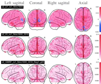
Because the multifractality parameter c2 is by definition negative, all plots below report−c2read as a quantification of the amount of multifractality. All plots were generated using nilearn (nilearn.github.io). The classical linear fit, univariate Bayesian and spatially regularized Bayesian estimates are reported and compared. They are labelled respectively as LF (for Linear Fit), as IG (for the use of an Inverse Gaussian prior in Bayesian inference) and GaMRF (for the use of a GaMRF prior for spatial regularization).
Because the present work intends to be a proof-of-principle contribution, and for the sake of clarity in
com-Left sagittal Coronal Right sagittal Axial
Fig. 1. Resting state(−c2)-maps estimated from the LF, IG and GaMRF
procedures (top to bottom).
menting the result, results are reported here for a single individual arbitrarily chosen (subject-level analysis). Similar findings were observed when analyzing other subjects.
Resting-state analysis.Fig. 1 compares estimates computed from resting-state data. A first obvious outcome is related to the fact that the range of estimated −c2 is very large for the LF estimates. This is a direct consequence of the fact that LF estimates show poor estimation performance with notably very large variance for small sample size, as is the case for fMRI signals (≃ 500 samples). Also estimates are both positive and negative because the LF procedure does not force a priori the estimate of c2 to be non-positive. A positive c2, as observed in the occipi-tal cortex (primary visual areas, blue areas in Fig. 1 top row), hence actually indicates the absence of multifractality. Conversely, the IG and GaMRF estimates of c2 naturally vary in a much narrower and same range, validating the theoretically documented significant decrease in estimation variance [16]. These two estimators both clearly indicate significant multifractality in the resting-state networks, and specifically in the default mode network (posterior cingulate cortex, bilateral angular gyri, clearly visible (dark red) in axial view in Fig. 1[bottom]). Prominent scale-free dynamics in the DMN was already reported from resting-state fMRI data in [3] but this finding was only supported by large Hurst exponent estimates (i.e.H ≃1). Here, we provide evidence for richer, i.e. multifractal, resting-state brain dynamics in the DMN, which is much more enhanced using the GaMRF estimate for c2. This clearly illustrates the direct benefit of the GaMRF spatial regularization procedure, which can be regarded as a first attempt to multivariate multifractal analysis, as opposed to the LF or IG based analyses that remain univariate. Also, the values retrieved by the Bayesian estimators are lower in magnitude due to the involved priors which tend to shrinkc2 to zero when the likelihood is less informative.
Left sagittal Coronal Right sagittal Axial
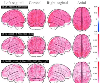
Fig. 2. Task (3-back run)(−c2)-maps estimated from the LF, IG and
GMRF estimators (from top to bottom).
the 3-back run that provides the most salient differences between estimators. The 1-back and 2-back runs lead to similar conclusions but with less pronounced amplitude.
A global comparison of all estimates in Fig. 2 (task) versus those of Fig. 1 (rest) shows an overall increase of multifractality during task, an interesting resultper se, which confirms earlier findings [8], [9]. Fig. 2 further confirms that the LF estimator yields estimates spread in a much larger range, hence having a large variance, a consequence being that it is difficult to assess variations of multifractality across the brain. Conversely, the IG and GaRMF show much better contrast and indicate clear differences between regions showing multifractality (large −c2) and other with little or no multifractality (c2≃0). Notably, the GaMRF procedure shows significant multifractality in the bilateral parietal re-gions (cf. sagittal and axial views in Fig. 2[bottom]) which belong to the working memory network (WMN), and are hence obviously involved into the designed task. Large multifractality is also reported in the occipital cortex due to the delivery of visual stimuli and in the cerebellum due to its connections with sensory systems.
V. CONCLUSIONS AND FUTURE WORKS
The present contribution showed the benefits and relevance of performing a multivoxel regularization for the estimation of multifractal attributes for the characterization of scale-free temporal dynamics in fMRI data, as opposed to the classical and so far state-of-the-art approach that consists in performing multifractal analysis independently on each voxel and hence not exploiting voxel geometrical proximity. Interestingly, this multivoxel-based regularization of multi-fractal analysis shows an increase of multimulti-fractality during task in brain regions (Working Memory Network) involved in performing the task. This is a confirmation of earlier findings showing their temporal dynamics to appear more irregular and more bursty (more multifractality, larger|c2|) often accompanied with less global structure, or correlation
(lowerc1) (cf. e.g., [8], [9]). At rest, larger multifractality is also reported in the Default Mode Network confirming the predominance of scale-free dynamics in this circuit, as already reported in the literature. For the proof-of-principle and ease of exposition, results were reported here at the subject-level only. Group-level statistical analysis are being performed, and the analysis of the whole cohort should hopefully confirm that multifractal properties, well assessed by the spatially regularized approach proposed here, could be considered as a viable metrics for brain analysis purposes.
REFERENCES
[1] P. Ciuciu, P. Abry, C. Rabrait, and H. Wendt, “Log wavelet leaders cumulant based multifractal analysis of EVI fMRI time series: evi-dence of scaling in ongoing and evoked brain activity,”IEEE Journal
of Selected Topics in Signal Processing, vol. 2, no. 6, pp. 929–943,
2008.
[2] B. J. He, J. M. Zempel, A. Z. Snyder, and M. E. Raichle, “The temporal structures and functional significance of scale-free brain activity,” Neuron, vol. 66, no. 3, pp. 353–369, 2010.
[3] B. J. He, “Scale-free properties of the functional magnetic resonance imaging signal during rest and task,” The Journal of Neuroscience, vol. 31, no. 39, pp. 13786–13795, Sept. 2011.
[4] D. Van de Ville, J. Britz, and Ch. Michel, “EEG microstate sequences in healthy humans at rest reveal scale-free dynamics,”Proceedings of
the National Academy of Sciences of the United States of America,
vol. 107, no. 42, pp. 18179–84, 2010.
[5] N. Dehghani, C. Bedard, S. S. Cash, E. Halgren, and A. Des-texhe, “Comparative power spectral analysis of simultaneous elecroen-cephalographic and magnetoenelecroen-cephalographic recordings in humans suggests non-resistive extracellular media,” J Comput Neurosci, vol. 29, no. 3, pp. 405–421, 2010.
[6] P. Ciuciu, G. Varoquaux, P. Abry, S. Sadaghiani, and A. Kleinschmidt, “Scale-free and multifractal time dynamics of fMRI signals during rest and task,” Front Physiol, vol. 3, June 2012.
[7] P. Ciuciu, P. Abry, and B. J. He, “Interplay between functional connectivity and scale-free dynamics in intrinsic fMRI networks,”
Neuroimage, vol. 95, pp. 248–263, 2014.
[8] N. Zilber, P. Ciuciu, P. Abry, and V. van Wassenhove, “Modulation of scale-free properties of brain activity in MEG,” inProc. of the 9th
IEEE International Symposium on Biomedical Imaging, Barcelona,
Spain, 2012, pp. 1531–1534.
[9] N. Zilber, P. Ciuciu, P. Abry, and V. van Wassenhove, “Learning-induced modulation of scale-free properties of brain activity measured with MEG,” inProc. of the 10th IEEE International Symposium on
Biomedical Imaging, San Francisco, USA, 2013, pp. 998–1001.
[10] K. Gadhoumi, J. Gotman, and J.-M. Lina, “Scale invariance properties of intracerebral eeg improve seizure prediction in mesial temporal lobe epilepsy,” PloS one, vol. 10, no. 4, 2015.
[11] B. J. He, “Scale-free brain activity: past, present, and future,”Trends
in Cognitive Science, vol. 18, no. 9, pp. 480–487, 2014.
[12] V. Maxim, L. Sendur, J. Fadili, J. Suckling, R. Gould, R. Howard, and E. Bullmore, “Fractional Gaussian noise, functional MRI and Alzheimer’s disease,”Neuroimage, vol. 25, no. 1, pp. 141–158, 2005. [13] D. Veitch and P. Abry, “A wavelet based joint estimator of the param-eters of long-range dependence,” IEEE Transactions on Information
Theory, vol. 45, no. 3, pp. 878–897, 1999.
[14] H. Wendt, P. Abry, and S. Jaffard, “Bootstrap for empirical multifractal analysis,”IEEE Signal Proc. Mag., vol. 24, no. 4, pp. 38–48, 2007. [15] S. Combrexelle, H. Wendt, N. Dobigeon, J.-Y. Tourneret, S.
McLaugh-lin, and P. Abry, “Bayesian estimation of the multifractality parameter for image texture using a whittle approximation,” IEEE T. Image
Proces., vol. 24, no. 8, pp. 2540–2551, 2015.
[16] S. Combrexelle, H. Wendt, Y. Altmann, J.-Y. Tourneret, S. McLaugh-lin, and P. Abry, “Bayesian estimation for the local assessment of the multifractality parameter of multivariate time series,” in
Proc. European Signal Processing Conference (EUSIPCO), Budapest,