Vol. 10 (2016) 3548–3578 ISSN: 1935-7524
DOI:10.1214/16-EJS1196
Simple approximate MAP inference for
Dirichlet processes mixtures
Yordan P. Raykov∗ Aston University e-mail:[email protected] Alexis Boukouvalas∗ University of Manchester e-mail:[email protected] and Max A. Little
Aston University and MIT e-mail:[email protected]
Abstract: The Dirichlet process mixture model (DPMM) is a ubiquitous, flexible Bayesian nonparametric statistical model. However, full probabilis-tic inference in this model is analyprobabilis-tically intractable, so that computa-tionally intensive techniques such as Gibbs sampling are required. As a result, DPMM-based methods, which have considerable potential, are re-stricted to applications in which computational resources and time for in-ference is plentiful. For example, they would not be practical for digital signal processing on embedded hardware, where computational resources are at a serious premium. Here, we develop a simplified yet statistically rigorous approximate maximum a-posteriori (MAP) inference algorithm for DPMMs. This algorithm is as simple as DP-means clustering, solves the MAP problem as well as Gibbs sampling, while requiring only a frac-tion of the computafrac-tional effort.†Unlike related small variance asymptotics (SVA), our method is non-degenerate and so inherits the “rich get richer” property of the Dirichlet process. It also retains a non-degenerate closed-form likelihood which enables out-of-sample calculations and the use of standard tools such as cross-validation. We illustrate the benefits of our algorithm on a range of examples and contrast it to variational, SVA and sampling approaches from both a computational complexity perspective as well as in terms of clustering performance. We demonstrate the wide ap-plicabiity of our approach by presenting an approximate MAP inference method for the infinite hidden Markov model whose performance contrasts favorably with a recently proposed hybrid SVA approach. Similarly, we show how our algorithm can applied to a semiparametric mixed-effects regression model where the random effects distribution is modelled us-ing an infinite mixture model, as used in longitudinal progression mod-elling in population health science. Finally, we propose directions for fu-ture research on approximate MAP inference in Bayesian nonparamet-rics.
∗These authors contributed equally to this work.
†For freely available code that implements the MAP-DP algorithm for Gaussian mixtures
seehttp://www.maxlittle.net/.
MSC 2010 subject classifications:Primary 62F15; secondary 62G86.
Keywords and phrases:Bayesian nonparametrics, clustering, Gaussian mixture model.
Received May 2016.
1. Introduction
Bayesian nonparametric(BNP) models have been successfully applied to a wide range of domains but despite significant improvements in computational hard-ware, statistical inference in most BNP models remains infeasible in the context of large datasets, or for moderate-sized datasets where computational resources are limited. The flexibility gained by such models is paid for with severe de-creases in computational efficiency, and this makes these models somewhat im-practical. This is an important example of the emerging need for approaches to inference that simultaneously minimize both empirical risk and computational complexity (Bousquet and Bottou,2008). Towards that end we study a simple, statistically rigorous and computationally efficient approach for the estimation of BNP models that significantly reduces the computational burden involved, while keeping most of the model properties intact. In this work, we concentrate on inference for theDirichlet process mixture model (DPMM) and for the infi-nite hidden Markov model (iHMM) (Beal et al., 2002) but our arguments are more general and can be extended to many BNP models.
DPMMs are mixture models which use theDirichlet process(DP) (Ferguson, 1973) as a prior over the mixing distribution of the model parameters. The data is modeled with a distribution with potentially infinitely many mixture com-ponents. The DP is an adaptation of the discrete Dirichlet distribution to the infinite, uncountable sample space. Where the Dirichlet distribution is formed over a continuousK-element sample space, ifK→ ∞we obtain the DP. A draw from a DP is itself a probability distribution. A DP is the Bayesian conjugate prior to the empirical probability distribution, much as the discrete Dirichlet distribution is conjugate to the categorical distribution. Hence, DPs have value in Bayesian probabilistic models because they are priors over completely gen-eral probability distributions. DPs can be also used as building blocks for more complex hierarchical models; an example being the thehierarchical DP hidden Markov model (HDP-HMM) for time series data, obtained by modeling the tran-sition density in a standard HMM with ahierarchical Dirichlet process (HDP) (Teh et al.,2006).
An interesting property of DP-distributed functions is that they are discrete in the following sense: they are formed of an infinite, but countable mixture of Dirac delta functions. Since the Dirac has zero measure everywhere but at a single point, the support of the function is also a set of discrete points. This dis-creteness means that draws from such distributions have a non-zero probability of being repeats of previous draws. Furthermore, the more often a sample is re-peated, the higher the probability of that sample being drawn again – an effect known as the “rich get richer” property (known aspreferential attachmentin the
network science literature (Barab´asi and Albert,1999)). This repetition, coupled with preferential attachment, leads to another valuable property of DPs: sam-ples from DP-distributed densities have a strong clustering property whereby
N draws can be partitioned intoK representative draws, whereK≤N andK
is not fixeda-priori.
Inference in probabilistic models for which closed-form statistical estimation is intractable, is often performed using computationally demanding Markov-chain Monte Carlo(MCMC) techniques (Neal,2000a; Teh et al.,2006; Van Gael et al.,2008), which generate samples from the distribution of the model param-eters given the data. Despite the asymptotic convergence guarantees of MCMC, in practice MCMC often takes too long to converge and this can severely limit the range of applications. A popular alternative is to cast the inference problem as an optimization problem for which variational Bayes (VB) techniques can be used. Blei and Jordan (2004) first introduced VB inference for the DPMM, but their approach involves truncating the variational distribution of the joint DPMM posterior. Subsequently, collapsed variational methods (Teh et al.,2008) reduced the inevitable truncation error by working in a reduced-dimensional parameter space, but they are based on a sophisticated family of marginal likelihood bounds for which optimization is challenging. Streaming variational methods (Broderick et al.,2013a) obtain significant scaling by optimizing local variational bounds on batches of data visiting data points only once, but as a result they can easily become trapped in poor local fixed points. Similarly, stochastic variational methods (Chong et al., 2011) also allow for a single pass through the data, but sensitivity to initial conditions increases substantially. Alternatively, methods which learn memoized statistics of the data in a single pass (Hughes and Sudderth, 2013; Hughes et al., 2015) have recently shown significant promise.
Daum´e (2007) describe a related approach for inference in DPMM based on a combinatorial search that is guaranteed to find the optimum for objective func-tions which have a specific computationally tractability property. As the DPMM complete data likelihood does not have this particular tractability property, their algorithm is only approximate for the DPMM, and this also makes it sample-order dependent. On the other hand, Dahl (2009) describe an algorithm that is guaranteed to find the global optimum inN(N+ 1) computations, but only in the case of univariate product partition models with non-overlapping clusters. By contrast, our approach does not make any further assumptions beyond the model structure and being derived from the Gibbs sampler does not suffer from sample-order dependency. Wang and Dunson (2011) present another approach for fast inference in DPMMs which discards the exchangeability assumption of the data partitioning and instead assumes the data is in the correct ordering. Then a greedy, repeated “uniform resequencing” is proposed to maximize a pseudo-likelihood that approximates the DPMM complete data likelihood. This procedure does not have any guarantees for convergence even to a local optima. Zhang et al. (2014) extend the SUGS algorithm introducing a variational ap-proximation of the cluster allocation probabilities. This allows replacement of the greedy allocation updates with updates of an approximation of the
alloca-tion distribualloca-tion. However, this extension also lacks optimality guarantees and is mostly useful in streaming data applications.
Broderick et al. (2013b) propose a general approach to solving the MAP problem for a wide set of BNP models by forcing the spread of the likelihood of BNP models to zero. By making some additional simplifying assumptions, this approach reduces MCMC updates to a fast optimization algorithm that con-verges quickly to an approximate MAP solution. However, this small variance asymptotic (SVA) reasoning breaks many of the key properties of the underly-ing probabilistic model: SVA applied to the DPMM (Kulis and Jordan, 2012; Jiang et al., 2012) loses the rich-get-richer effect of the infinite clustering, as the prior term over the partition drops from the likelihood; and degeneracy in the likelihood forbids any kind of rigorous out-of-sample prediction and thus, for example, cross-validation. Roychowdhury et al. (2013) impose somewhat more flexible SVA assumptions to derive an optimization algorithm for infer-ence in the infinite hidden Markov model (iHMM). Although this approach overcomes some of the drawbacks of SVA Broderick et al. (2013b), the algo-rithm departs from the assumptions of the underlying probabilistic graphical model. The method is shown to be efficient for clustering time dependent data, but essentially no longer has an underlying probabilistic model. Furthermore, Roychowdhury et al. (2013) demonstrate that there is more than one way of applying the SVA concept to a given probabilistic model, and therefore, under different choices of SVA assumptions, one obtains entirely different inference algorithms that find different structures in the data, even though the under-lying probabilistic model remains the same. For example, HDP-means (Jiang et al., 2012) in the context of time series, and the alternative SVA approach of Roychowdhury et al. (2013) optimize different objective functions, even though they address inference for identical probabilistic models. To clarify this and other issues, we present a novel, unified exposition of the SVA approach in Section 4, highlighting some of its deficiencies and we show how these can be overcome using the non-degenerate MAP inference algorithms proposed in this paper.
In Section2we review the collapsed Gibbs sampler for DPMMs and in Section 3we show how the collapsed Gibbs sampler may be exploited to produce simpli-fied MAP inference algorithms for DPMMs. As with DP-means it provides only point estimates of the joint posterior. However, while DP-means follows the close relationship between K-means and the (finite) Gaussian mixture model
(GMM) to derive a “nonparametric K-means”, we exploit the concept of iter-ated conditional modes (ICM) (Kittler and F¨oglein,1984). Experiments on both synthetic and real-world datasets are used to contrast the MAP-DP, collapsed Gibbs, DP-means and variational DP approaches in Section5. In Section6 we demonstrate how the MAP DPMM approach can be extended to the iHMM and contrast it to the hybrid SVA approach of Roychowdhury et al. (2013) in a simulation study. Finally, we demonstrate an application of our new algorithm to a hierarchical model of longitudinal health data in Section 7 and conclude with a discussion of future directions for this MAP approach for BNP models in Section8.
2. Collapsed Gibbs sampling for Dirichlet process mixtures
The DPMM is arguably the most popular Bayesian nonparametric model which extends finite mixture models to the infinite setting by use of the DP prior. In this work we will restrict ourselves to mixture models with exponential family distribution data likelihoods. We will denote by X the full data ma-trix formed of the observed data points xi which are D-dimensional vectors
xi = (xi,1, . . . , xi,d, . . . , xi,D), N0 is the concentration parameter of the DP
prior andG0 is its base measure. The DPMM is then often written as:
G ∼ DP (N0, G0)
ϑi|G i.i.d.∼ G, i= 1, . . . , N (2.1) xi|ϑi ∼ F(xi;ϑi), i= 1, . . . , N
where G is a mixing distribution drawn from a DP; ϑ are the atoms of G
which take repeated values andF is the distribution of each data point given its atom. We can also write the mixing distribution G in terms of mixture weightsπand the distrinct values taken fromϑdenoted withθ,G=∞k=1πkδθk
and xi ∼ ∞
k=1πkF(θk), where δ(·) denotes the Dirac delta function. The
probability of the data follows an infinite mixture distribution and because this likelihood is not available in closed form, a Gibbs sampling procedure is not tractable. A widely used approach to overcome this issue is to collapse the mixture weights and model the data in terms of the cluster indicator variables
z1, . . . , zN: (z1, . . . , zN) ∼ CRP (N0, N) θ1, . . . , θK|z i.i.d. ∼ G0 (2.2) xi|z, θ ∼ F(xi;θzi), i= 1, . . . , N
where to simplify notation we denote z = (z1, . . . , zN) and θ = (θ1, . . . , θK);
CRP stands for the Chinese restaurant process which is a discrete stochastic process over the space of partitions, or equivalently a probability distribution over cluster indicator variables. It is strictly defined by the integer N (number of observed data points) and a positive, real concentration parameter N0. A draw from a CRP has probability:
p(z1, . . . , zN) = Γ (N0) Γ (N+N0) N0K K k=1 Γ (Nk) (2.3)
with indicators z1, . . . , zN ∈ {1, . . . , K}, where K is the unknown number of items andNk =|{i:zi=k}|is the number of indicators taking value k, with
K
k=1Nk = N. For any finite N we will have K ≤ N and usually K will be
much smaller thanN, so the CRP returns apartition ofN elements into some smaller number of groupsK. The probability over indicators is constructed in a sequential manner using the following conditional probability:
p(zn+1=k|z1, . . . , zn) = Nk N0+n ifk= 1, . . . , K N0 N0+n otherwise (2.4) By increasing the value ofnfrom 1 toN and using the corresponding condi-tional probabilities, we obtain the joint distribution over indicators from Equa-tion (2.3), p(z1, . . . , zN) = p(zN|z1, . . . , zN−1)p(zN−1|z1, . . . , zN−2)× · · · × p(z2|z1).
The probability density function ofxi∼F(xi;θzi) associated with the
com-ponent indicated by the value ofzi, is an exponential family distribution: p(xi|θzi) = exp (g(xi), θzi −ψ(θzi)−h(xi)) (2.5)
where g(.) is the sufficient statistic function, ψ(θzi) = log
exp(xi, θzi −
h(xi))dxi is the log partition function and h(xi) the base measure of the
dis-tribution. An important property of exponential family distributions is that the conjugate prior over the natural parametersθk ∼G0exists and can be obtained in closed form:
p(θ|z,τ, η) = exp (θ,τ −ηψ(θ)−ψ0(τ, η)) (2.6)
where (τ, η) are the prior hyperparameters of the base measureG0, ψ0 is base measure of the parameter distribution. From Bayesian conjugacy, the posterior
p(θk|X,τk, ηk) will take the same form as the prior where the prior hyperpa-rametersτ andη will be updated toτk=τ+
j:zj=kg(xj) andηk=η+Nk.
Inference can be accomplished via collapsed Gibbs sampling, presented as Algorithm 3 in Neal (2000b). This MCMC algorithm iteratively samples each component indicatorzi fori= 1, . . . , N, conditional on all others, until
conver-gence:
p(zi =k|xi, z−i)∝
Nk,−ip(xi|τk,−i, ηk,−i) for existingk
N0p(xi|τ, η) for some newk=K+ 1
(2.7) where the subscript−idenotes the removal of pointifrom consideration,z−i=
{z1, . . . , zi−1, zi+1, . . . , zN} and p(xi|τ, η) is the posterior predictive density
of point i obtained after integrating out the cluster parameters, p(xi|τ, η) =
p(xi|θ)p(θ|τ, η)dθ. Examples of posterior predictive densities for different
exponential family likelihoods are presented in AppendixB.
3. Introducing MAP-DP: A novel approximate MAP algorithm for collapsed DPMMs
In this section we propose a novel DPMM inference algorithm based on it-eratively updating the cluster indicators with the values that maximize their posterior (MAP values). The cluster parameters are integrated out. This algo-rithm can be also seen as an an “exact” version of themaximization-expectation
(M-E) algorithm presented in Welling and Kurihara (2006). It is exact in the fol-lowing sense: while the M-E algorithm is a kind of VB and as with VB makes a
factorization assumption which departs from the underlying probabilistic model purely for computational simplicity and tractability purposes, our algorithm is derived directly from the Gibbs sampler for the probabilistic model. Therefore, our algorithm does not introduce or require this simplifying factorization as-sumption. In Section 3.1 we describe how parameter inference for the DPMM is accomplished and in Section3.2we consider out-of-sample prediction.
3.1. Inference
As a starting point, we consider the DPMM introduced in Section 2. In our algorithm, we iterate through each of the cluster indicatorsziand update them with their respective MAP values. For each observation xi, we compute the
negative log probability for each existing clusterkand for a new clusterK+ 1:
qi,k=−logp(xi|z−i,X−i, zi =k,τk,−i, ηk,−i) (3.1)
qi,K+1=−logp(xi|τ, η) (3.2)
where terms independent of k may be omitted as they do not change with k. For each observationxi we compute the aboveK+ 1-dimensional vectorqiand
select the cluster number according to the following:
zi= arg min
k∈{1,...,K,K+1}
[qi,k−logNk,−i]
whereNk,−i is the number of data points assigned to clusterk, excluding data
pointxi and, for notational convenience, we defineNK+1,−i ≡N0.
The algorithm proceeds to the next observationxi+1by updating the cluster
component statistics to reflect the new value of the cluster assignment zi and
remove the effect of data pointxi+1. To check convergence of the algorithm we
compute the negative log of the complete data likelihood:
p(x, z|N0) = N i=1 K k=1 p(xi|zi)δ(zi,k) p(z1, . . . , zN) (3.3)
where δ(zi, k) is the Kronecker delta and p(z1, . . . zN) is the CRP partition
function (Pitman, 1995) given in Equation (2.3). We show in Algorithm 1 all the steps involved in approximately maximizing this complete data likelihood.
It is worth pointing out that unlike MCMC approaches, MAP-DP does not increase the negative log of the complete data likelihood at each step and as a result is guaranteed to converge to a fixed point. Where the convergence reached by MCMC sampling is convergence in distribution to the stationary posterior measure, the convergence of MAP-DP is only to local maxima of the posterior measure and so it is much quicker to reach. The main disadvantages with this are that the solution at convergence is only guaranteed to be a local maximum and that information about the whole distribution of the posterior is lost. Multiple restarts using random permutations of the data can be used to overcome poor local maximum. With MAP-DP it is possible to learn all model hyperparameters as we discuss in AppendixA and this is a strong advantage over the fast SVA approaches.
Input: x1, . . . ,xN: data;N0>0: concentration parameter, >0: convergence threshold; (τ, η): cluster prior parameters;ψ0(.): prior log partition function; g(.): sufficient statistic function.
Output:z1, . . . , zN: cluster assignments,K: number of clusters.
K= 1, zi= 1, for alli∈1, . . . , N; Enew=∞; repeat Eold=Enew; fori∈1, . . . , Ndo fork∈1, . . . , Kdo qi,k= ψ0 τ+j:z j=k,j=ig(xj), η+Nk,−i −ψ0 τ+j:z j=kg(xj), η+Nk end qi,K+1=ψ0(τ, η)−ψ0(τ+g(xi), η+ 1); zi= arg mink∈1,...,K,K+1
qi,k−logNk,−i
; ifzi=K+ 1then K=K+ 1; end end Enew=Kk=1i:z i=kqi,k−Klog (N0)− K k=1log Γ (Nk); untilEold−Enew< ;
Algorithm 1:MAP-DP: Exponential Families
3.2. Out-of-sample prediction
To compute the out-of-sample likelihood for a new observationxN+1we consider
two approaches that differ in how the indicatorzN+1 is treated:
1. Mixture predictive density.The unknown indicatorzN+1can be integrated
out resulting in a mixture density:
p(xN+1|N0, z,X) = K+1
k=1
p(zN+1=k|N0, z,X)p(xN+1|z,X, zN+1=k) (3.4)
The assignment probabilityp(zN+1=k|z, N0,X) is NN0+Nk for an existing
cluster and N0
N0+N for a new cluster. The second term corresponds to the
predictive distribution of point N+ 1 according to the predictive densi-ties p(xN+1|z,X,τk, ηk, zN+1=k) and p(xN+1|τ, η, zN+1=K+ 1) for
an existing and new cluster respectively.
2. MAP cluster assignment. We can also use a point estimate for zN+1 by picking the minimum negative log posterior of the indicator
p(zN+1|xN+1, N0, z,X), equivalently: zNMAP+1 = arg min
k∈{1,...,K,K+1}[−logp(xN+1|z,X, zN+1=k)
where p(xN+1|z,X, zN+1=k) and p(zN+1 =k|N0, z,X) are exactly as
above. This approach is useful for clustering applications when we are interested in estimating zMAP
N+1 explicitly. Once the MAP assignment for
pointN+ 1 is updated, we estimate the probability ofxN+1 given that it
belongs to the component pointed byzMAP N+1,p
xN+1|z,X, zMAPN+1
. The first (marginalization) approach is used in Blei and Jordan (2004) and is more “robust” as it incorporates the probability of all cluster components while the second (modal) approach can be useful in cases where only a point cluster assignment is needed. Integrating over variablezN+1for more robust estimation ofxN+1is an example of the well studied process known asRao-Blackwellization
(Blackwell, 1947) which is often used in Bayesian inference for improving the quality of statistical estimation of uncertainty.
Even when using the first approach however, the mixture density is still computed assuming point assignments for the training data z1, . . . , zN. There-fore the predictive density obtained using MAP-DP will be comparable to the one obtained using Gibbs sampler inference only when the sufficient statistics
N1, . . . NK of the categorical likelihood for the assignment variables estimated from a Gibbs chain are similar to the ones estimated from the modal esti-mates for z1, . . . , zN. Empirically, we have observed this often to be the case.
Furthermore, we have noticed that the predictive density for popular (with a lot of points) cluster components tend to be well approximated by MAP-DP where the effect of the smaller cluster components diminishes when using only modal estimates for z. Note that the DPMM usually models data with a lot of inconsistent small spurious components (Miller and Harrison, 2013), those and any consistent components with small effect are likely to be ig-nored when using MAP-DP as we later show in Section 5.1. To summarize, using only modal estimates for the cluster assignments we are likely to in-fer correctly only larger components which have a large effect on the model likelihood and which will also affect the estimated predictive density accord-ingly.
4. Another look at small variance asymptotics (SVA)
The novel MAP-DP algorithm presented here has the “flavor” of an SVA-like algorithm, but there are critical differences and advantages, which we discuss in detail in this section.
Firstly, some background to the SVA approach is required. There exists a well known connection between the expectation-maximization (E-M) algorithm for the finiteGaussian Mixture Model(GMM) andK-means. That is, by assuming a GMM with equal variance, spherical (diagonal) component covariance matrices, we can obtain K-means from the E-M algorithm for the corresponding GMM by shrinking the component variances in each dimension to 0. This approach is more recently referred to as thesmall variance asymptotic (SVA) derivation of theK-means algorithm (Bishop,2006, page 423).
Using Bregman divergences Dφ(·) (see Appendix C), Banerjee et al. (2005)
has extended the SVA reasoning to any exponential family finite mixtures and
K-means like clustering procedures can be derived. Banerjee et al. (2005) showed that the likelihood of pointxifrom componentkgiven the component parameter θk and the posterior of parameter θk given its posterior hyperparameters can be rewritten using Bregman divergences as:
p(xi|θk) = exp (−Dφ(xi,μk)fφ(xi)) p(θk|τk, ηk) =exp −ηDφ τk ηk ,μk gφ(τk, ηk) (4.1) whereφis the Legendre-conjugate function ofψ,fφ(xi) = exp (φ(xi)−h(xi))
and gφ(τ, η) = exp (ηφ(θ)−ψ0(τ, η)) with h(·) andψ0(·) denoting the base
measure of the corresponding distributions andμis the expectation parameter satisfying μ = ∇ψ(θ). Kulis and Jordan (2012) extended this more compact form to the nonparametric DPMM and with some further assumptions derived a nonparametricK-means like algorithm that we now review in detail. Consider the DPMM above (with non-integrated component parameters), but with a scaled exponential family likelihood ˜F
˜
θ that is parameterized by a scaled natural parameter ˜θ=ξθand log-partition function ˜ψ
˜ θ =ξψ ˜ θ/ξ for some
ξ >0. Further assume that the prior parameters of the natural parameter are also scaled appropriately, such that ˜τ = τξ and ˜η= ηξ. It is then straightforward to see that the conjugate prior of ˜ψ will be also scaled and so ˜φ =ξφ. Then Jiang et al. (2012) have shown that ˜F
˜
θ has the same mean as F(θ), but scaled covariance, cov
˜
θ = cov (θ)/ξ. Let us also assume thatN0is a function
ofξ,η andτ, taking the form:
N0= gφ˜ τ ξ, η ξ 2π ξ+η D/2 ξD −1 exp (−ξλ) (4.2) for some free parameterλthat will replace the concentration parameter in the new formulation; D denotes dimension of the data and is unrelated toDφ(·).
Then we can write the scaled exponential family DPMM as ξ → ∞ and as a consequence cov
˜
θ
→ 0. Following Jiang et al. (2012) we can write out the Gibbs sampler probabilities in terms ofDφ(·) (see AppendixC) after canceling outfφ˜(xi) terms from all probabilities:
p(zi=k|z−i,xi, ξ,μ) = Nk,−iexp (−ξDφ(xi,μk)) Cxiexp (−ξλ) + K j=1Njexp −ξDφ xi,μj p(zi =K+ 1|z−i,xi, ξ,μ) = Cxiexp (−ξλ) Cxiexp (−ξλ) + K j=1Njexp −ξDφxi,μj
whereCxiapproaches a positive, finite constant for a givenxiasξ→ ∞and we
both of the above probabilities will become binary (take on the values 0 or 1) as
ξ→ ∞ and so allK+ 1 values will be increasingly dominated by the smallest value of{Dφ(xi,μ1), Dφ(xi,μ2), . . . , Dφ(xi,μK), λ}. That is, the data point
xi will be assigned to the nearest cluster with Bregman divergence at mostλ.
If the closest mean has a divergence greater then λ, we create a new cluster containing onlyxi.
The posterior distribution over the cluster parameters for some componentk
is concentrated around the sample mean of points assigned to that component
1 Nk
Nk
i=1xi as ξ→ ∞, so we update the cluster means with the sample mean
of data points in each cluster, as with the corresponding parameter update step in K-means. The resulting algorithm approximately minimizes the following objective function over (z, μ):
K k=1 i:zi=k Dφ(xi,μk) +λK (4.3)
Similar objective function omitting the penalty termλKwas utilized in Banerjee et al. (2005) in the context of finite mixture models.
Although this algorithm is straightforward, it has various drawbacks in prac-tice. The most troublesome is that the functional dependency between the con-centration parameter and the covariances destroys the rich-get-richer property of the DPMM because the counts of assignments to componentsNk,−ino longer
influence which component gets assigned to an observed data point. Only the geometry in the data space matters. A new cluster is created by comparing the parameterλagainst the distances between cluster centers and data points so that the number of clusters is controlled by the geometry alone, and not by the number of data points already assigned to each cluster. So, for high-dimensional datasets, it is not clear how to choose the parameter λ. By con-trast, in the DPMM Gibbs sampler, the concentration parameter N0 controls
the rate at which new clusters are produced in a way which is, for fixed ge-ometries, independent of the geometry. Another problem is that shrinking di-agonal covariances to zero variance means that the component likelihoods be-come degenerate Dirac point masses which causes likelihood comparisons to be meaningless since the likelihood becomes infinite. So, we cannot choose parameters such as λ using standard model selection methods such as cross-validation.
While Jiang et al. (2012) can be seen as a nonparametric extension of the well known derivation of K-means from the (E-M) algorithm, Roychowdhury et al. (2013) have suggested an alternative SVA approach in the context of the iHMM. Herein we review their approach in the context of DPMMs and discuss their original formulation in Section 6.3. Instead of simply reducing the diago-nal likelihood covariance to 0 variance in each dimension, Roychowdhury et al. (2013) represent the categorical distribution over the latent variablesz1, . . . , zN
in the more general exponential family form. The conditional distribution of the cluster indicator for pointigiven the mixture weights is given by:
whereπ= (πk)Kk=1is the vector of mixture weights. Written in this form now we
can also scale the variance of the categorical distribution over z. Furthermore, Roychowdhury et al. (2013) assume an additional dependency (which is not part of the DPMM) between the distribution of the cluster indicators and the com-ponent mixture distribution, in order for their diagonal variances to approach 0 simultaneously. That is, while Jiang et al. (2012) change the underlying DPMM structure only by assuming shrinking covariance, Roychowdhury et al. (2013) modify the underlying DPMM such that the conditional independence of the cluster parameters and cluster indicators no longer holds. Let us replace the distribution from Equation (4.4) with a scaled one:
p(zi|π) = exp
−ξDφˆ (zi,π) b˜
φ(zi) (4.5)
where ˜φ= ˆξφwhich will keep the same mean as in Equation (4.4). Then follow-ing Roychowdhury et al. (2013) we assume that the likelihood ˜F
˜
θ is scaled with ξ for which the equality ˆξ = λ1ξ holds for some real λ1. Now, taking
ξ → ∞would result in the appropriate scaling. After taking the limit and re-moving the constant terms we obtain the objective function of this new SVA approach: K k=1 i:zi=k Dφ(xi,μk) +λ1Dφ(zi, πk) +λK (4.6)
which is optimized with respect to (z, μ, π), and where Dφ(zi, πk)−logπk. Optimization with respect to the mixture weights results in the empirical prob-ability for the cluster weightsπk =NNk. So, this objective function then can be
rewritten as: K k=1 i:zi=k Dφ(xi,μk)−λ1logNk N +λK (4.7)
The E-M procedure that tries to optimize this objective function computes, for each observation xi, the K divergences to each of the existing clusters: Dφ(xi,μk) fork = 1, . . . , K. Then, it takes into account the number of data
points in each component by adjusting the corresponding divergence for clusterk
by subtractingλ1logNk
N . After computing these adjusted distances, observation
xi is assigned to the closest cluster unlessλis smaller than all of these adjusted
distances, in which case a new cluster is created. Then the cluster means are updated with the sample mean of observations assigned to each cluster, and in addition we now have to update the countsN1, . . . , NK.
By contrast to the SVA algorithm proposed by Jiang et al. (2012), the SVA algoritm of Roychowdhury et al. (2013) no longer clusters the data purely on geometric considerations, but also takes into account the number of data points in each cluster. In this respect the method has greater flexibility, but at the same time, unlike MAP-DP, we can see that SVA algorithms do not actually-optimize the complete data likelihood of the original underlying probabilistic
DPMM which motivates their derivation. By assuming additional ad-hoc de-pendencies between the likelihood distribution and the distribution over the indicator variables, SVA algorithms effectively start from a different underlying probabilistic model which is not explicitly given. This makes them less princi-pled and more heuristic than the MAP-DP algorithm we present here. So, while SVA algorithms are quite simple, they sacrifice several key statistical principals including structural interpretability and the existence of an underlying proba-bilistic generative model.
5. DPMM experiments
This section provides some empirical results so that we can compare the perfor-mance of MAP-DP against existing approaches.
5.1. Synthetic CRP parameter estimation
We examine the performance of the MAP-DP, collapsed Gibbs, DP-means (Kulis and Jordan, 2012) and variational DP (Blei and Jordan, 2004) on CRP-parti-tioned, non-spherical Gaussian data in terms of estimation error and compu-tational effort. We generate 100 samples from a two-dimensional DPMM. The partitions are sampled from a CRP with fixed concentration parameterN0= 3
and data size N = 600. Gaussian component parameters are sampled from a normal-Wishart (NW) prior with parameters μ0 = [2,3], c0 = 0.5, ν0 =
30,Λ0 =
2 1 1 3
. This prior ensures a combination of both well-separated and overlapping clusters. We fit the model using MAP-DP, variational DP and Gibbs algorithms using the ground truth model values for the NW prior and theN0used to generate the data. Convergence for the Gibbs algorithm is tested
using the Raftery diagnostic (q= 0.025, r= 0.1, s= 0.95) (Raftery and Lewis, 1992). We use a high convergence acceptance tolerance ofr= 0.1 to obtain less conservative estimates for the number of iterations required. We use the most likely value from the Gibbs chain after burn-in samples (1/3 of the samples) have been removed.
Clustering estimation accuracy is measured using thenormalized mutual in-formation (NMI) metric (Vinh et al.,2010). The parameterλfor DP-means is set using a binary search procedure such that the algorithm gives rise to the cor-rect number of partitions (see AppendixD). This approach favours DP-means as it is given knowledge of the true number of clusters which is not available to the other algorithms. For variational DP we set the truncation limit to ten times the number of clusters in the current CRP sample.
Both MAP-DP and Gibbs achieve similar clustering performance in terms of NMI whilst variational DP and DP-means have lower scores (Table1). MAP-DP
Table 1
Performance of clustering algorithms on the CRP mixture experiment (Section5.1). Mean and standard deviation (in brackets) reported across 100 CRP mixture samples. The range
of the NMI is[0,1]with higher values reflecting higher clustering accuracy. Gibbs-MAP MAP-DP DP-means Variational DP Training set NMI 0.81 (0.1) 0.82 (0.1) 0.68 (0.1) 0.75 (0.1)
Iterations 1395 (651) 10 (3) 18 (7) 45 (18)
requires the smallest number of iterations to converge with the Gibbs sampler requiring, on average, 140 more iterations and DP-means 1.8 times. In Figure 5.1(a) the median partitioning1 is shown in terms of the partitioning Nk/N
and the number of clusters. As expected, when using a CRP prior, the sizes of the different clusters vary significantly with many small clusters containing only a few observations. MAP-DP and variational DP fail to identify the smaller clusters whereas the Gibbs sampler is able to do so to a greater extent. This is a form of underfitting where the algorithm captures the mode of the partitioning distribution but fails to put enough mass on the tails (the smaller clusters). The NMI scores do not reflect this effect as the impact of the smaller clusters on the overall measure is minimal. The poorer performance of the DP-means algorithm can be attributed to the non-spherical nature of the data as well as the lack of reinforcement effect that leads to underestimation of the larger clusters and overestimation of the smaller clusters.
This poor performance of DP-means is confirmed by modifying the CRP ex-periment to sample from spherical clusters (Figure 5.1(b)). The CRP is again sampled 100 times and the MAP-DP algorithm attains NMI scores of 0.88 (0.1) and DP-means scores NMI 0.73 (0.1). As the clusters are spherical, the lower performance of the DP-means algorithms is solely explained by the lack of re-inforcement effect.
Fig 5.1. CRP mixture experiment; distribution of cluster sizes, actual and estimated using different methods. Cluster number ordered by decreasing size (horizontal axis) vs Nk
N (vertical
axis).
1For each inference method, this is the median paritioning in terms of NMI out of the 100 DPMM sampled datasets.
Table 2
Clustering performance of DP-means, MAP-DP, and Gibbs samplers on UCI datasets, measured using NMI (two standard deviations in brackets), averaged over all runs. Higher
NMI is better.
DP-means Gibbs MAP-DP
Wine(178 observations, 13 dimensions) 0.42 0.71 (0.06) 0.86 Iris(150 observations, 4 dimensions) 0.76 0.75 (0.06) 0.76 Breast cancer(683 observations, 9 dimensions) 0.75 0.72 (0.01) 0.71 Soybean(266 observations, 35 dimensions) 0.36 0.45 (0.00) 0.40 Pima(768 observations, 8 dimensions) 0.03 0.14 (0.01) 0.07 Vehicle(846 observations, 18 dimensions) 0.21 0.10 (0.02) 0.15
5.2. UCI datasets
Next, we compare DP-means, MAP-DP and Gibbs sampling on six UCI machine learning repository datasets (Blake and Merz,1998):Wine;Iris;Breast cancer;
Soybean;Pima and Vechicle. We assess the performance of the methods using the same NMI measure as in Section5.1. Class labels in the datasets are treated as cluster numbers.2 There is either no or a negligibly small number of missing values in each of the data sets. The data types vary between datasets and features: Wine consists of integer and real data; Iris contains real data; Breast cancer consists of integer and categorical data; Soybean is categorical data; Pima is real data and Vehicle consists of integer data.
As in Section 5.1 we stop the Gibbs sampler using the Raftery diagnostic (Raftery and Lewis,1992). For DP-means, we chooseλto give the true number of clusters in the corresponding dataset (Kulis and Jordan,2012). For the Gibbs algorithm, we report the NMI of the most likely clustering from the whole chain of samples (Table2). We also report the two standard deviations of the NMI computed at each sample of the chain after burn-in.
On almost all of the datasets (5 out of 6), MAP-DP is comparable to, or even better than, the Gibbs sampler, and on 4 out of 6 datasets it performs as well as or better than DP-means (Table2). DP-means performs well on lower-dimensional datasets with a small number of clusters. In higher dimensions, it is more likely for the clusters to be elliptical rather than spherical and in such cases the other algorithms outperform DP-means because of the more flexible model assumptions. In addition, for higher dimensional data it is more often the case that the different features have different numerical scaling, so the squared Euclidean distance used in DP-means is inappropriate. Furthermore, MAP-DP and the Gibbs sampler are more robust to smaller clusters due to the longer tails of the Student-T predictive distribution (AppendixB) and the rich-get-richer effect of existing clusters assigned many observations. DP-means is particularly sensitive to geometric outliers and can easily produce excessive numbers of spurious clusters for poor choices ofλ.
2We do not assess “Car” and “Balance scale” datasets used in Kulis and Jordan (2012) because they consist of a complete enumeration of 6 and 4 categorical factors respectively, and it is not meaningful to apply an unsupervised clustering algorithm to such a setting.
Table 3
Iterations required to achieve convergence for the DP-means and MAP-DP algorithm, and the Gibbs sampler, on datasets from the UCI repository.
DP-means Gibbs MAP-DP
Wine 19 2,365 11 Iris 8 1,543 5 Breast cancer 8 939 8 Soybean 14 1059 9 Pima 20 1,189 17 Vehicle 12 939 9
Even though MAP-DP only gives a point estimate of the full joint posterior distribution, MAP-DP can in practice achieve higher NMI scores than for Gibbs due to MCMC convergence issues.
We emphasize that these algorithms attempt to maximize the model fit rather than maximize NMI. The true labels would not be available in practice and it is not always the case that maximizing the likelihood also maximizes NMI. Fur-thermore, if we choose the model hyperparameters for each dataset separately, by minimizing the negative log likelihood with respect to each parameter, higher NMI can been achieved, but choosing empirical estimates for the model param-eters simplifies the computations.
In all cases, the MAP-DP algorithm converges more rapidly than the other al-gorithms (Table3). The Gibbs sampler takes, typically, greater than 1000 more iterations than MAP-DP to achieve comparable NMI scores. The computational complexity per iteration for Gibbs and MAP-DP is comparable, requiring the computation of the same quantities. This makes the Gibbs sampler significantly less efficient than MAP-DP in finding a good labeling for the data. The com-putational price per iteration for DP-means can often be considerably smaller than MAP-DP or the Gibbs sampler, as one iteration often does not include a scan through allN data points. This occurs because the scan ends when a new cluster has to be created, unlike MAP-DP and Gibbs. But, this also implies that DP-means requires more iterations to converge than MAP-DP.
6. MAP-DP for infinite hidden Markov models
The simplicity of MAP-DP makes it straightforward to extend to more complex nonparametric models, such as the popular time series hidden Markov model. Mirroring the approach taken in Section3, we can obtain an approximate MAP algorithm for the infinite HMM (Beal et al., 2002) (also known as the HDP-HMM (Teh et al., 2006)) for modeling sequential, time-series data.
HMMs can be seen as a generalization of finite mixture models where the cluster indicators that denote mixture component assignments are not indepen-dent of each other, but related through a Markov process. That is, each data pointxtof a sequence observations (x1, . . . ,xT) is drawn independently of the
other observations when conditioned on the state variable for time t, zt. The
de-fines a mixture model for one of the values of the categorical distribution on the states. The current stateztindexes a specific row of the transition matrix, with
probabilities in this row serving as the mixing proportions for the choice of the next statezt+1. Therefore the HMM does not involve a single mixture model, but rather a set of different mixture models, one for each value of the current state. (Beal et al.,2002) showed that if we replace the mixture models with a set of DPs, one for each value of the current state, a nonparametric variant of HMM is obtained that allows an unbounded set of states. In order to obtain sharing of available states across the sequence, the atoms associated with the state-conditional DPs are shared and so the transition matrix is modeled with an HDP (Teh et al.,2006).
Let us denote the base measure of the HDP byH where we restrictH to an exponential family distribution (for Bayesian conjugacy);N0 andM0 arelocal
and global concentration parameters; zt−1 indicates the state chosen at time t−1. The HDP-HMM can then be written as:
G0∼DP (M0, H) Gzt−1 ∼DP (N0, G0) ϑtzt−1 ∼Gzt−1 xt∼F ϑtzt−1
where distribution over the dataFϑtzt−1
is a mixture distribution with mixing distributionGzt−1 overϑdetermined by the state pointed by zt−1. We can also
write the mixing distribution in terms of transition matrixπ and base measure atomsθ,Gzt−1 =
∞
k=1πzt−1kδθkandxt∼
∞
k=1πzt−1F(θk) for allG1, . . . , GK.
The rows of the transition matrixπdenote the mixture weights for each of the local DPs, while θ1, . . . , θK are the shared atoms which are the same across
G1, . . . , GK, whereKdenotes the number of represented components, which in a nonparametric setting is unknown. Theglobal DP is then characterized with
G0=∞k=1κkδθk where the elements ofκare the mixture weights of this global
DP.
6.1. Gibbs sampler
As in the case of DPMMs (Section2), exact inference is not available and Gibbs sampling is a standard choice for inference. A popular approach is based upon thedirect assignment sampling approach for the HDP (Teh et al.,2006), where the cluster parameters θ and the transition matrixπ are integrated out. The resulting Gibbs sampler then iterates between sampling the state indicators z
and the global mixture weights κ. The mixture weights can be sampled from the corresponding Dirichlet posterior:
κ1, . . . , κK, κK+1∼Dirichlet (M1, . . . , MK, M0) (6.1) whereMkcounts how many times the transition to statekhas been drawn from
the global DP and some extra effort is needed to compute the global counts; we only use the assignmentsztof a point to its corresponding state and those
assign-ments are used to compute the local DP counts, Npk=|{t:zt−1=p, zt=k}|,
that count how many times a transition occurred from statepto statek. Letmpk
be the count of how many times transitions from state pto state k have been drawn as a new transition from the global DP. We then haveMk=pmpk. It is straightforward to see that if Npk= 0 then mpk= 0, because the first time
the transition occurs from state pto statek, it is sampled from the global DP. Furthermore, the count mpk will be limited by Npk, as at most all transitions from state pto statek are sampled from the global DP. We can then use the
Polya urn sampling scheme underlying the transition probability from state p
to statekto sample mpk:
p(zt+1=k|zt=p)∝
N−zt+1
pk −1 for an existing transition fromptok N0κk for a new transition fromptok
(6.2) Due to the exchangeability of rows in the transition matrix, we can sam-ple from Equation (6.2) sequentiallyNpk times, gradually increasing Npk, and
keeping count of how many times the transition from the second term has been sampled. The recorded count mpk is unbiased and can be marginalized overp
to obtainMk (Van Gael,2012).
In order to update the state indicators, fort= 1, ..., T we sampleztfrom the corresponding probability:
p(zt|X, z−t, κ)∝p(xt|z−t, zt,X)p(zt|z−t, κ) (6.3) where z−t denotes all indicators excluding the one for data point t. The first
term is the posterior predictive distribution of data point xt given its state
and it will be obtained after integrating out the state parametersθ assuming a conjugate prior for the exponential family likelihood. The resulting distribution is computed in the same way as in Section3.1:
p(xt|. . .)∝exp ⎛ ⎝ψ0 ⎛ ⎝τ+ j:zj=k g(xj), η+Nk ⎞ ⎠ −ψ0 ⎛ ⎝τ+ j:zj=k,j=t g(xj), η+Nk,−t ⎞ ⎠ ⎞ ⎠ (6.4)
To compute the second term recall that DPs for each row of the transition matrix are independent, given the shared base measure κ. Then if Nk· denotes
can write: p(zt=k|z−t, κ)∝ ⎧ ⎪ ⎪ ⎪ ⎪ ⎪ ⎪ ⎪ ⎪ ⎨ ⎪ ⎪ ⎪ ⎪ ⎪ ⎪ ⎪ ⎪ ⎩ Nz−t−t1k+N0κk N−t kzt+1+N0κzt+1 Nk−·t+N0 fork≤K, zt−1=k Nz−t−t1k+N0κ Nkzt+1−t +1+N0κzt+1 Nk−·t+N0+1 forzt−1=zt+1=k Nz−tt −1k+N0κk N−t kzt+1+N0κzt+1 Nk−·t+N0+1 forzt−1=k=zt+1 N0κkκzt+1 fork=K+ 1 (6.5)
6.2. MAP-DP for iHMMs
In our proposed iterative MAP approach, we sweep through the latent variables and at each iteration update them one at a time with their respective MAP values. Following the direct assignment construction presented in the previous section, the random variables to be updated are the global DP mixture weights
κand the state indicatorsz. The mode of the Dirichlet posterior is available in closed form for concentration parameterM0≥1, so we can updateκusing:
κk= M·M−kK−−11 for an existing statek= 1, . . . , K κK+1=M·M−0K−1−1 for a new state
(6.6) where M· = Kk=0Mk. The counts mpk can be computed by numerical
opti-mization of the corresponding distribution over partitions provided in (Anto-niak,1974). However, the expression involves Stirling numbers of the first kind which may be numerically challenging to compute when the method is applied to time series with a large number of observations. One approach to avoid this issue is using Equation (6.2) to sequentially compute the corresponding counts. In order to update the state indicators, we sweep through each observation xtand then compute the negative log probability for each existing statekand
for a new stateK+ 1:
qt,k =−logp(xt|zt=k,X−t)−logp(zt=k|z−t, κ)
qt,K+1= −logp(xt|τ, η)−log (N0κK+1κzt+1)
where again and without losing generality, we can omit the terms independent ofk. For each observation in the time series, we compute theK+ 1-dimensional vectorqtand select the state number according to:
zt= arg min
k∈{1,...,K,K+1}
qt,k (6.7)
As with the MAP-DP case, the algorithm proceeds to the next point in the time series xt+1 by updating the state sufficient statistics to reflect the new
value of the cluster assignmentztand remove the effect of data pointxt+1. The
not increase the NLL. However, when the Polya urn scheme in Equation (6.2) is used to compute the global DP counts its stochastic nature will result in minor fluctuations in the model NLL. The algorithm still falls into a local optima, but minor fluctuations occur between iterations. As the NLL is significantly more influenced by the likelihood terms logp(xt|zt=k,X−t) and the assignment
probabilities, stopping the scheme at the local minima is straightforward.
6.3. SVA for iHMMs
Jiang et al. (2012) propose an alternative inference algorithm for efficient estima-tion of iHMMs based on the SVA approach (Secestima-tion4). Mirroring the simplified inference assumptions explained in Section4, Jiang et al. (2012) have extended the SVA approach to HDP mixtures and so can be readily applied for infer-ence in the HDP-HMM model. The resulting algorithm extends the objective function derived for the simpler DPMM with an additional term penalizing the number of transitions leading out of each state:
min z,μ,K T t=1 Kglobal k=1 Dφ(xt, μk) +λ1 Kglobal p=1 Kplocal+λ2Kglobal (6.8)
In the case of the iHMM, Kplocal denotes the number of states for which a transition from state pexists, and Kglobal denotes the total number of repre-sented states in the finite time series. Then λ2 penalizes the creation of new
states, whileλ1 controls how likely new transitions are between existing states.
As in the DPMM SVA algorithm (Section 4), standard model selection tech-niques cannot be applied to select the values of λ1 and λ2 and reinforcement
terms have been stripped away. Alternatively, introducing some additional as-sumptions which imply an entirely ad-hoc coupling between the state indicator distribution and the data likelihood probabilities, (Roychowdhury et al.,2013) derives an SVA algorithm that optimizes the following objective function:
min K,Z,μ,T T t=1 Kglobal k=1 Dφ(xt, μk)−λ T t=2 Kglobal k=1 logNzt−1k Nzt−1· +λ1 Kglobal p=1 Kplocal+λ2Kglobal (6.9) (Roychowdhury et al., 2013) also introduces a further algorithm, unrelated to Gibbs sampling, that attempts to optimize this objective function whilst also taking advantage of dynamic programming. The method is referred to as asymp-iHMM in our synthetic experiment below.
6.4. Synthetic study
We compare the performance of the Gibbs, SVA and MAP-DP algorithms for iHMMs on synthetically generated 3-dimensional data from a five-state HMM with Gaussian data models. The five Gaussian components are parameterized
Table 4
NMI and number of iterations to convergence for different iHMM inference algorithms. ‘+’ indicates convergence was not obtained.
NMI Iterations Gibbs sampler 0.77 2500+
asymp-iHMM 0.58 12
MAP-iHMM 0.62 13
with isotropic means μd
1, μd2, μd3, μd4, μd5
= [0.2,1.1,1.8,3.4,4.8] for d= 1,2,3, each with shared spherical covariance σI3 where σ = 0.9. At each time step
the HMM has 0.96 probability of self-transition and equal probability to tran-sition to any of the remaining four states. 4000 data points are generated and performance of the algorithms is measured using the NMI between the true and estimated state assignments. The Gibbs sampler is evaluated for the state assignments that maximize the model likelihood. As shown in Table 4, MAP-iHMM performs similarly to asymp-MAP-iHMM from (Roychowdhury et al., 2013) whilst keeping the underlying probabilistic iHMM model intact and retaining a non-degenerate complete data likelihood.
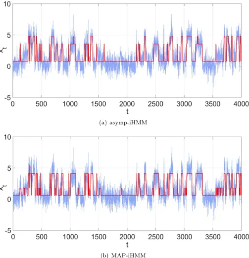
Inferring states in this data is difficult due to overlapping observation likeli-hood models, and we find that the Gibbs sampler significantly outperforms both point estimation approaches, but at an even greater computational cost than for the simpler DPMM. This example illustrates the computational challenges of using MCMC inference for more complex hierarchical models. In Figure6.1 we observe that the state sequence obtained by MAP and SVA is similar and underestimates the true number of states.
7. MAP-DP for semiparametric mixed effects models
Hierarchical modeling is commonly used in the analysis of longitudinal health data. A particular model that is widely used in practice is the linear mixed effects model:
yi = Xiβi+i (7.1)
βi ∼ P
whereyi the observation vector for individuali∈ {1, . . . , N}, i∼ N
0, τ−1 σ I
is the subject-specific observation noise withτσthe within-subject precision and
P the distribution of therandom effects βi (Dunson,2010).Xi are the inputs
for the random effectsβiand the fixed effect regression parameters are equal to the mean of the distributionP. The distributionP is commonly specified to be Gaussian due to analytical tractability and computational simplicity. However, the assumption of normality is seldom justified and the assumptions of symmetry and unimodality are often found to be inappropriate (Dunson,2010).
Semiparametric mixed effects models have been proposed to relax the nor-mality assumption by placing a DPMM prior on P (Kleinman and Ibrahim, 1998). However, inference for such models is usually performed using MCMC
Fig 6.1. Synthetically generated HMM data is in blue. The red line is the estimated state centroids associated with each point, where centroids have been estimated using (a) asymp-iHMM and (b) MAP-asymp-iHMM.
requiring large computational resources and careful tuning of algorithmic pa-rameters. This makes MCMC approaches particularly difficult to implement on large data sets. The increasing availability of large longitudinal data sets war-rants the investigation of computationally efficient inference approaches such as MAP-DP. Here in order to construct a semiparametric mixed effects model, we will use an iterative MAP algorithm similar to MAP-DP above with the only difference of not integrating out the component parameters.
We construct the model by first placing a DPMM prior on βi in Equation (7.1). As we are interested in the interpretation of the clusters we do not collapse out the cluster parameters and the update steps described for MAP-DP are slightly altered (as in non-collapsed Gibbs) where the random effects βi are
substituted for the individual data points xi; an additional step updating the
component means and precisions also needs to be included. Two further steps are needed to update the random effects βi and within-subject precision τσ.
The conditionalp(βi|τσ, zi =k,μk,Rk) for the random effectsβi is:
NβiτσXTi Xi+Rk −1 τσXTiyi+Rkμk ,τσXTi Xi+Rk −1 (7.2) where the conditioning is on the assigned clusterkwith meanμk and precision Rk. We place a conjugate Gamma prior on the within-subject precision τσ ∼
Gamma (aσ2, bσ2) allowing for the calculation of the conditional posterior:
p(τσ|B, aσ2, bσ2) = Gamma τσ aσ2+ N 2, bσ2+ 1 2 N i=1 (yi−Xiβi) T (yi−Xiβi) (7.3)
where B is the collection of all random effects (βi)N
i=1. The modes of both
conditionals needed for MAP-DP are easily calculated in addition to the negative log likelihood necessary to check for convergence.
7.1. English longitudinal survey of ageing
We apply the semiparametric mixed effects model above to the English lon-gitudinal survey of ageing (ELSA), a large longitudinal survey of older adults aged over 50 in the United Kingdom. ELSA is a multi-purpose health study which follows individuals aged 50 years or older (Netuveli et al.,2006). Collected health-related factors include clinical, physical, financial and general well-being. Of primary interest is the effect of the different factors onquality of life (QoL) measured using a compound measure of several health and socio-economic indi-cators. The ELSA survey has been conducted in five waves spanning ten years. In this preliminary study we look at the response of 6,805 individuals across all 5 waves.
We wish to check the hypothesis that measures of cognition such as memory and executive mental function, as estimated by verbal fluency, are useful pre-dictors of QoL and whether they are more informative than standard measures of depression and activities of daily living (ADL) that have been found to be statistically significant predictors of QoL (Netuveli et al., 2006). We propose to answer these two questions via selection of two models with different sets of covariates. The first model includes depression and ADL as inputs whereas the second model includes measures of cognitive ability, specifically prospective memory and verbal fluency. The models are assessed using 5-fold cross-validation and computing the average held-out likelihood (Equation (3.4) in Section3.2). The model that includes ADL and depression as covariates achieves a signif-icantly lower average held-out likelihood than the competing model containing cognitive measures suggesting that ADL and depression are more informative predictors of QoL than the cognitive measures we considered (Table5).
Table 5
Cross-validation average held-out likelihood for two models. Cognitive measures Depression + ADL
0.364 3.834
The average elapsed time for fitting the models using MAP inference is 11.05 seconds and 16.29 seconds3. For comparison we performed inference using a
truncated DP random effects model with MCMC and 100,000 iterations to en-sure convergence on less than half of the data (3,000 individuals) and the result-ing time to convergence is in excess of five hours makresult-ing inference on larger data sets impractical. On the other hand, the rapid inference obtained using MAP-DP enables a wide array of diagnostic and validation methods to be exploited, which suggests the approach can be scaled up to very large datasets.
8. Discussion and future directions
We have presented a simple algorithm for inference in DPMMs based on non-degenerate MAP, and demonstrated its efficiency and accuracy by comparison to the ubiquitous Gibbs sampler, variational DP, and the SVA algorithms. The attractiveness of SVA lies in the simplicity and scalability of the resulting algo-rithms but as we have shown, it entails significant structural departures from the DPMM as well as removing from the modeler’s arsenal standard tools of model comparison and selection. We believe our approach is highly relevant to applications since, unlike SVA, it retains the preferential attachment (rich-get-richer) property while needing two orders of magnitude fewer iterations than Gibbs. Unlike SVA, the out-of-sample likelihood may be computed allowing the use of standard model selection and model fit diagnostic procedures. Lastly, this non-degenerate MAP approach does not require the approximation inherent to the factorization assumptions of VB.
As with most MAP methods, MAP-DP can get trapped in local minima, however, standard heuristics such as multiple random restarts can be employed to mitigate this risk. This would increase the total computational cost of the algorithm somewhat but even with random restarts it would still be far more efficient than the Gibbs sampler.
Although not reported here due to space limitations, we point out that differ-ent implemdiffer-entations of the Gibbs sampler can lead to differdiffer-ent MAP inference algorithms for DPMMs. For example, different MAP procedures can be derived from the different Gibbs samplers presented in (Neal, 2000b). In general, we have found these alternative algorithms to be less robust in practice, as they do not integrate over the uncertainty in the cluster parameters. However, when such assumptions are justified, our MAP approach can be readily applied to different constructions of the DPMM, for example to allow for non-conjugate choice of priors (extending Algorithm 7 (Neal,2000b)).
3The reported runtimes for MAP-DP and MCMC were obtained on Matlab R2013a (8.1.0.604) 64-bit (glnxa64), i7-2600 CPU with 3.40GHz processor, ubuntu PC.