Using Survey Data on Inflation Expectations in
the Estimation of Learning and Rational
Expectations Models
Arturo Ormeño
CES
IFO
W
ORKING
P
APER
N
O
.
3552
C
ATEGORY6:
F
ISCALP
OLICY,
M
ACROECONOMICS ANDG
ROWTHA
UGUST2011
An electronic version of the paper may be downloaded
• from the SSRN website: www.SSRN.com
• from the RePEc website: www.RePEc.org
CESifo
Working Paper No. 3552
Using Survey Data on Inflation Expectations in
the Estimation of Learning and Rational
Expectations Models
Abstract
Do survey data on inflation expectations contain useful information for estimating
macroeconomic models? I address this question by using survey data in the New Keynesian
model by Smets and Wouters (2007) to estimate and compare its performance when solved
under the assumptions of Rational Expectations and learning. This information serves as an
additional moment restriction and helps to determine the forecasting model for inflation that
agents use under learning. My results reveal that the predictive power of this model is
improved when using both survey data and an admissible learning rule for the formation of
inflation expectations.
JEL-Code: C110, D840, E300, E520.
Keywords: survey data, learning models, inflation expectations, Bayesian econometrics.
Arturo Ormeño
Department of Economics
University of Amsterdam (UvA)
Amsterdam / The Netherlands
[email protected]
First draft: March 2009; This draft: 28th March 2011
This paper is part of my Ph.D. dissertation at Universitat Pompeu Fabra. I thank Fabio
Canova, Kristoffer Nimark, Marco del Negro, Jose Dorich, Christina Felfe, Jordi Gali, Albert
Marcet, Krisztina Molnar, Sergey Slobodyan, Robert Zymek and the participants of the
Society for Economic Dynamics (SED) 2009 Annual Meeting, European Econometric
Society 2009 Annual Meeting, the XIV Workshop on Dynamic Macroeconomics organized
by Universidad de Vigo, the 8th Macroeconomic Policy Research Workshop on DSGE model
organized by Magyar Nemzeti Bank and the Centre for Economic Policy Research (CEPR),
and the Macroeconomic student seminar at UPF for useful comments and suggestions. I am
grateful to Sergey Slobodyan for sharing his MATLAB codes. Any comments and/or
suggestions are welcome at [email protected].
2
1. Introduction
Survey data on inflation expectations have received significant attention in monetary economics. In particular, this information has been applied to a variety of cases including use as a proxy for expected inflation in the estimation of the Phillips curve (Adam and Padula (2011), Nunes (2010)); in calibrations of hybrid models with both backward-looking and forward-looking expectations (Roberts (1997, 1998)); and to test rational expectations and informational rigidities (Mankiw et al. (2003), Coibion and Goridnichenko (2010)). However, few studies have used this information in the estimation of a dynamic stochastic general equilibrium (DSGE) model. I attempt to fill this gap by including survey data on inflation expectations in the estimation of one of the benchmark models for empirical analysis, namely the medium-size New Keynesian DSGE model developed by Smets and Wouters (2007) (the SW model).
I estimate this model using two alternative methods to model expectations: first, I consider the benchmark assumption about expectations formation, the Rational Expectations (RE) hypothesis, and then I consider learning. There are two reasons for choosing these two alternatives.
First, even though the SW model explains the evolution of inflation and has higher predictive power than Bayesian VARs, it fails to match the evolution of survey data on inflation expectations when solved under the RE assumption and estimated with the standard set of macroeconomic indicators (see Figure 1). Therefore, the additional moment restriction implied by the use of survey data on inflation expectation in the estimation of the model might arguably affect the parameter estimates.
Second, as indicated by Slobodyan and Wouters (2009a,b), when assuming learning, the estimation of the SW model leads to different outcomes depending on the forecasting model used.1 This result reflects the main criticism of learning: that it relies heavily on the researcher’s arbitrary selection of the forecasting model that agents may use to generate their expectations. In order to address this criticism, I employ survey data to determine the forecasting model that agents are most likely to use to predict inflation.
1
Slobodyan and Wouters (2009a,b) point out that the dynamics of the model under learning do not tend to deviate from the RE outcomes when the forecasting models are compatible with the solution under RE, but they deviate significantly when small forecasting models are considered.
3 Figure 1
Inflation expectations: survey data and model-implied expectations under RE
1970 1975 1980 1985 1990 1995 2000 2005 0 0.5 1 1.5 2 2.5 3 Survey data RE Inflation
Notes: The model-implied inflation expectations are obtained using the Kalman-filtered estimates at each set of parameter values that conforms the posterior distributions. The grey area represents the distance between the 5th and 95th percent confidence bands.
Additionally, I use survey data on inflation expectations to pursue a model-comparison analysis between the RE and learning solutions. Similar to Del Negro and Eusepi (2010), I determine how the use of survey data in the estimation alters the relative fit of the two alternative assumptions of expectations formation.
Our findings reveal the following. First, according to the model comparison analysis, the RE and learning solutions of the SW model fit the standard macroeconomic series in similar way. However, this situation changes once survey data are incorporated into the analysis: the learning solution is now clearly preferred because it is flexible enough to match the increases and decreases in inflation expectations during the late 1970s and the early 1980s. Second, the better performance of learning can be explained mainly by the selection of a small forecasting model for inflation and a high speed of learning. As previously mentioned, survey data are employed to determine the specification of this forecasting model.
Third, through an analysis of the parameter estimates, I find that the additional moment restriction, which represents the inclusion of the survey data on inflation expectations, results in a higher persistence of exogenous shocks under RE. This occurs despite the fact that the SW model incorporates nominal frictions such as price stickiness and indexation. In contrast, price indexation and the learning process itself are the main sources of inflation persistence under
4
learning. Additionally, under learning, the use of survey data reduces the time-variability of the coefficients of the agents´ forecasting model. As a result, most of the stronger and more persistent responses of inflation to exogenous shocks are concentrated in the 1970s. In the same vein as Boivin and Giannoni (2006), I observe that the unexpected monetary policy shocks had many more destabilizing effects on inflation during the 1970s than afterwards. To date, few studies have incorporated survey data into the estimation of a DSGE model. Del Negro and Eusepi (2010) use survey data on inflation expectations to discriminate between a model with imperfect information about a time-varying inflation target, similar to Erceg and Levin (2003), and a model where agents have perfect information about this target. Additionally, Carboni and Ellison (2009) incorporate the Greenbook unemployment forecast into the estimations implemented by Sargent et al. (2006). By incorporating this forecast, Carboni and Ellison remove the Federal Reserve´s volatile and unrealistic beliefs about unemployment-inflation dynamics. In contrast to these studies, I do not only exploit the additional moment restrictions implied by the use of survey data, but I also employ this information to “discipline” how the forecasting model for inflation is selected under learning. The remainder of the paper is organized as follows. In the next section, I summarize the main features of the model, characterize its solution under both RE and learning, and discuss the specific learning setup employed in this study. Section 3 presents the series of macroeconomic indicators, the measurement equations and the prior distributions used in the Bayesian estimation. Section 4 describes the forecasting model used for the learning specification and the results of the model comparison analysis. It also details the evaluation of the changes in the parameter estimates obtained when using survey data in the estimation of the SW model and their effects on the relative importance of the sources of inflation persistence, the composition of inflation expectations, and the Impulse-Response functions analysis. Section 5 contains some robustness exercises. Lastly, Section 6 concludes and outlines possible avenues for future research.
2. The model and its solution under the RE assumption and learning
Our estimation is based on a New Keynesian model, which is similar to the SW model. I make only one modification, which will be explained below. The optimization problem of the households, firms and the government as well as the equilibrium conditions are described in detail in the Online Appendix. Readers interested in more of the details of the model are encouraged to refer to SW.
5
In the remainder of this section, I describe the model’s participants and its frictions, how participants’ decisions depend on forecasts of future variables, the minor modification to the SW model, and the representation of the model solution under the assumptions of RE and learning.
2.1 Model participants, main frictions, and forward variables
The New Keynesian model by SW is based on a neoclassical growth model augmented with several frictions affecting both nominal and real decisions of households and firms. Households maximize a utility function that depends on both the consumption of goods and the amount of labor supplied over an infinite lifetime horizon. Consumption in the utility function enters relative to a time-varying external habit variable. This feature, together with the possibility of both consumption and labor smoothing that is possible through the purchasing and selling of a one-period bond, generates that current consumption depends on past and expected future consumption, on current and expected future hours worked and on the ex-ante real interest rate of this bond. Households also rent capital services to firms and decide how much capital to accumulate given the capital adjustment costs they face. This friction creates a link between investment, the market value of the capital stock and past and expected future investment. In addition, the arbitrage condition for the value of the capital stock implies that this stock reacts positively to both its expected future value and the expected future real rental rate of capital, but negatively to the ex-ante real interest rate. Variations in the rental price of capital affect the level of utilization of the capital stock, which can be adjusted at increasing costs.
Labor is differentiated by a union that determines wages by taking into account the existence of nominal rigidities à la Calvo (1983). Thus, given the possibility of not being re-optimized within one period but only partially indexed to past inflation, wages depend on past and expected future wages and inflation. Firms produce differentiated goods, decide on the amount of labor and capital services to hire, and set prices. Prices are also affected by Calvo-type rigidity and when not re-optimized they are partially indexed to past inflation rates. Therefore, prices are set as a function of current and expected future marginal costs, but are also determined by the past inflation rate.
Lastly, there is an empirical monetary policy reaction function: the policy-controlled interest rate is adjusted in response to inflation and to changes in the level of output from one period to another. In the original SW specification, the monetary policy rule does not react to growth
6
in output but to the output gap (i.e., the difference between the output obtained under nominal rigidities and under flexible prices). This modification allows me to avoid the estimation of a parallel economy under flexible prices, which reduces the number of forward variables in the model considerably. As reported by Slobodyan and Wouters (2009a), I find that this modification does not affect the results obtained by SW.
The model contains 13 endogenous variables: output,y; consumption,
c
; investment,i
; value of the capital stock ,Qk; installed stock of capital,k ; stock of capital,k; inflation,π
; capital utilization rate,u; real rental rate on capital,rk; real marginal cost,mc; real wages,w; hours worked, L; and interest rate, R. In addition, seven exogenous autoregressive processes characterize the stochastic part of the model, with each of them including an iid-normally distributed error.2 The model is de-trended with respect to the deterministic growth rate of the labor-augmenting technological progress and linearized around the steady-state of the de-trended variables. The set of equations that describes the linearized dynamism of this model can be represented using the following two equations:(1) Θ0E Yt t+1+ Θ1Yt+ Θ2Yt−1+ Ψ =et 0 and
(2) et = Γe te−1+ Γε
ε
t.Y is the vector that contains the 13 endogenous variables of the model, e is the vector of exogenous shocks, and
ε
is the vector of iid-normal innovations. Et( )⋅ is the expectations operator, which indicates that expectations can either be rational (for which I use Et( )⋅ ) or come from a learning process (represented by Eˆ ( )t ⋅ ). The matrices Θ0, Θ1, Θ2, and Ψcontain both the non-linear combinations of the parameters of the model and zeros elements. The zero elements in these matrices illustrate that the model does not include the expected future values or past values of all of the endogenous variables. Then, Γe is a diagonal matrix that contains the autoregressive coefficients of the exogenous shocks. Lastly, Γε is an identity
2
These shocks are the risk premium and the investment-specific technology shocks, which affect the inter-temporal margin; the wage and price mark-up shocks, which impact the intra-temporal margin; the exogenous spending and the monetary policy shocks; and the total factor productivity shock.
7
matrix that also incorporates one element that reflects the effect of a productivity innovation over the exogenous spending shocks.3
2.2 The Rational Expectation solution of the DSGE model
When dealing with expectations, researchers have traditionally adopted the RE assumption. This assumption implies that agents have perfect knowledge about the true stochastic process of the economy. There are several algorithms available to solve Equation (1) under the RE assumption. I use Uhlig (1999), although alternative algorithms include Blanchard and Kahn (1980), Binder and Pesaran (1997), Christiano (2002) and Sims (2002).
I focus on the case of determinacy and restrict the parameter space accordingly. The resulting law of motion takes the following form:
(3) Yt = Φ1REYt−1+ Φ2REet−1+ ΦRE3
ε
t.Equations (2) and (3) imply a state-space representation of the DSGE model that can be estimated with the Kalman filter, where the vector
[
Y e]
' can be viewed as a partially latent state vector.2.3 The learning solution of the DSGE model
Because the high level of cognitive ability and computational skill implied under the RE assumption are implausible in practice, researchers have developed models of imperfect knowledge and associated learning processes. One of the most popular learning mechanisms used in macroeconomics is a form of adaptive learning. Under this approach, agents use historical data to update their perceptions about how the economy works and to form their expectations about future variables using forecasting models that are updated whenever new data become available (see Evans and Honkapohja (2001)).
Before presenting the learning algorithm used in this study, it is important to note that the forward-looking nature of Equation (1) leads to a simultaneity problem in case the solution for
t
Y depends on the reduced form coefficients of the forecasting models that rely on information up to t. The standard way to overcome this problem is to assume that agents
3 SW include this element because in the estimation, exogenous spending includes net exports, which may be
8
make their forecast of Yt+1 based on estimates of the reduced-form coefficients from the period t-1.4 Thus, expectations adopt the following equation:
(4) E Yˆt t+1=
β
t′−1Xt, X ⊂[
1 Y e]
',where X is a vector that includes either all endogenous and exogenous variables of the model or only a subset of them. It may also include a constant term that signifies that agents use an observable, non-zero mean time series in their forecasting models.
β
t′−1 is a matrix of the linear combinations of the reduced-form coefficients that define the projection of Xt−2 over Yt−1.5In applied studies, the researcher arbitrarily chooses the forecasting model that agents use to form their expectations. All state variables of the model can be included to not depart far from the RE setup; exogenous shocks and variables that are not observed in reality can be excluded under the assumption that agents and the researcher have the same set of information. Moreover, one could include a subset of those observed variables by arguing that the overall fit of the model to the data would be better if they were included. One of the contributions of this study is to deviate from this arbitrary choice of the forecasting model by using survey data on inflation expectations to determine the actual forecasting models for inflation that agents are most likely to use.6
With respect to the estimation of
β
, the literature on learning commonly assumes that agents update the coefficients of their forecasting models using the constant-gain least squares (CG-LS) algorithm. Under CG-LS, the most recent observations receive higher weights in the least square estimation. More precisely, the weight decreases geometrically depending on the distance in time to the most recent observation. This learning mechanism implies that agents are concerned about structural changes of the economy, which is a realistic feature of any type of econometric estimation. Additionally, the CG-LS receives empirical support because it outperforms other recursive parameter updating algorithms such as recursive least squares
4 Alternatively, as indicated by Carceles-Poveda and Giannitsarou (2007), one may assume that Y
tis not included in the information set when forming expectations, i.e., that expectations are formed using data up to t-1.
5
Due to the use of observable time series in the forecasting model for inflation, the row of
β
′ related to inflation expectations includes linear combinations of the coefficients that define the projections among observable series (see derivations in subsection 4.1).6
9
and the Kalman filter for out-of-sample forecasting of inflation and output growth (see Branch and Evans (2006)).
The recursive expression for the estimate of
β
under the CG-LS conditional on information up to t is as follows:(5a)
β
t =β
t−1+g R( )
t −1X Yt(
t−β
t′−1Xt−1)
' and(5b) Rt=Rt−1+g X
(
t−1Xt′−1−Rt−1)
.In these equations, g represents the constant-gain parameter and Rt is the variance-covariance matrix of the regressors included in the forecasting model. The gain parameter refers to the relative weight of the most recent observation, and 1−g is the discount factor over less recent observations (in ordinary least squares, the gain is not a constant value but equals 1/t, where t is the position of the observation since the beginning of the sample). When g=0,
β
is constant and equal to the value that starts the recursion. Otherwise,β
changes with the arrival of new information. An important observation is that g is the only parameter that is added to the set of structural parameters of the model.Substituting Equation (4) in Equation (1) and using Equation (2), I get the following expression: (6) Yt = Φ0,Lt−1+ Φ1,Lt−1Yt−1+ Φ2,Lt−1et−1+ Φ3,Lt−1
ε
t.The matrices Φ0,Lt−1, Φ1,Lt−1, Φ2,Lt−1, and Φ3,Lt−1 are non-linear combinations of the parameters of the model and the reduced form coefficients of
β
t−1. The presence of these latter elements potentially makes these matrices time-varying.In sum, the state-space representation of the model estimated under learning consists of Equations (6) and (2). Equations (5a) and (5b) are additionally required to get estimates for
β
as well as some initial values for
β
and Rthat are necessary for the CG-LS algorithm.72.4 The learning setting used in this study
Survey data on inflation expectations are used to determine the forecasting model of inflation under learning. However, inflation is not the only variable that appears in expectations in the
7
10
model. Consumption, investment, hours worked, real wages, real rental rate on capital, and value of the capital stock also appear in expectations.8 Thus, in order to restrict the differences in the estimates of the model solved under RE and learning to the use of survey data on inflation expectations, I restrict the learning setting for the other variables’ expectations to be as close as possible to the RE setting.9 The latter implies that the forecasting models for these variables include as regressors the same variables that appear in their solution under the RE assumption (Equation 3). Furthermore, it implies that the initial values of the elements of
β
and Rrelated to these variables correspond to their respective rows of the matrices Φ1RE,
2 RE
Φ , and Φ3RE and to the unconditional second moments resulting from the RE solution.10,11 Additionally, the mentioned variables and inflation have separated CG-LS recursion processes; therefore, I consider two sets of equations (5a) and (5b), which implies two gain parameters. Because the forecasting model for inflation is incompatible with the RE solution for this variable, it is unfeasible to use the coefficients or the implied second moments of this solution as the initial conditions of the learning algorithm.12 For this reason, I use pre-sample estimates of
β
and Rto initialize the learning algorithm for inflation. As explained in Section 4, survey data on inflation expectations also play a role in the selection of these values.Finally, it is important to note that the learning dynamics in our model are incomplete because the model cannot converge with the RE equilibrium. This occurs for two reasons: first, the forecasting model for inflation is not compatible with the RE solution for this variable; second, the use of CG-LS in the presence of random shocks prevents the resulting dynamics from converging with the RE solution (Evans and Honkapohja (1995)). However, Honkapohja and Mitra (2003) show that incomplete learning with finite memory can have several attractive properties in standard frameworks. In particular, learning could be asymptotically unbiased in the sense that the mean of the first moment of the forecast is correct. Additionally, dynamics
8
This study focuses only on the use of survey data on inflation expectations. Three reasons motivate the selection of this series. First, survey data on inflation expectations have received significant attention in monetary economics (e.g., Roberts (1997,1998), Adam and Padula (2011), Nunes (2010), among others). Second, the quality of this information, jointly with survey data on output growth, has been evaluated by many studies (e.g., Ang et al. 2007). Third, the data are available for most of the sample of interest in this study.
9 Notice that it is not possible to have both learning and rational expectations at the same time. 10
In case the gain parameter for these variables is equal to zero, their forecasting model will be completely compatible with the RE solution, not only at the beginning but through the entire sample.
11
One advantage of choosing the initial conditions of the learning algorithm is that it avoids a significant increase in the number of parameters to be estimated (they more than duplicate the number of structural parameters of the model).
12
The use of pre-sample estimations of β and R related to the other variables that appear in expectations does not affect our results.
11
of incomplete learning result in good approximations of actual data, as argued by Marcet and Nicolini (2003) and Sargent (1999).13
3. Data and priors
The model is estimated using the same quarterly macroeconomic indicators for the United States (US) as in SW. In addition, I use survey data on inflation expectations provided by the Survey of Professional Forecasters (SPF). Even though it would be more appropriate to use survey data provided by the University of Michigan Surveys, which collects data directly from households because the model specifies that households make many of the important forecasts, I opt to use the SPF for two reasons. First, as pointed out by Del Negro and Eusepi (2010), the University of Michigan Surveys ask households about inflation in general; therefore it is impossible to relate this measure to a specific measurement of changes in prices, such as the Consumer Price Index or GDP deflator inflations. Second, the University of Michigan Surveys started collecting information about inflation expectations in quantitative form in 1978. As a consequence, it does not cover the years of the sample considered by SW, our benchmark reference. The SPF collects expectations on the future GDP deflator, which is a measurement compatible with the inflation series used by SW. Moreover, this series starts ten years earlier than the University of Michigan Surveys; thus, it covers almost completely the sample considered by SW.
Using the SPF, I calculate the median value of the quarterly one-period-ahead forecast for the percentage increase of the GDP deflator. The resulting series is referred to as “ , 1
e t t dlP + ”. Because this information is only available from 1968:4 onwards, this date marks the starting point of our sample. The sample covers all quarters until 2008:2. Further macroeconomic indicators considered are: the first difference of the logarithm of real GDP (“dlGDP”), real consumption (“dlCons”), real investment (“dlInv”), the real wage (“dlWage”), and the GDP deflator (“dlP”); the logarithm of hours worked (“lHours”); and the federal funds rate (“FedFunds”). Please refer to the Online Appendix for a detailed description of the data. The following set of measurement equations relates the mentioned macroeconomic indicators to the variables of the model when the survey data on inflation expectations are not included:
13
Marcet and Nicolini (2003) employ incomplete learning to explain the existence of hyperinflation processes in some Latin American countries. In a similar way, Sargent (1999) considers incomplete learning as an important element to explain the rises and decreases of inflation in the US.
12 (7) 1 1 1 1 ˆ ˆ ˆ ˆ ˆ ˆ ˆ ˆ ˆ ˆ ˆ t t t t t t t t t t t t t t t t t t y y dlGDP c c dlCons i i dlInv w w dlWage lHours l l dlP FedFunds r R
γ
γ
γ
γ
π
π
− − − − − − − − = + ,where
γ
represents the common quarterly trend growth rate, l represents the steady state hours worked,π
represents the quarterly steady state inflation rate, and r represents the quarterly steady state nominal interest rate.When survey data are incorporated into the estimation of the DSGE model, I need to add an additional measurement equation. Under the RE solution, this equation has the following form: (8a) ,e 1 ˆ 1 1,RE 2,RE t t t t t t t t dlP + =
π
+Eπ
+ +ζ
=π
+ Φ πY + Φ πe +ζ
. In this equation 1, RE π Φ and 2, RE πΦ symbolize the corresponding rows of Φ1RE and Φ2REin
Equation (3), that relate inflation to the vectors Y and e.
ζ
t represents an iid measurement error related to the surveys on inflation expectations. Hence, survey data are viewed as a noisy measure of actual expectations. Under learning, the extra measurement equation has the following form:(8b) dlPt te,+1=
π
+β
π′,t−1Xt+ζ
t,where
β
π′,t−1 is the row corresponding toβ
t′−1 in Equation (4). In both this equation and the previous one, I am implicitly assuming that inflation and inflation expectations have the same steady state.The structural model contains 38 parameters. Of these, 33 are estimated, while the remaining 5 are fixed at the values used in SW.14 The learning estimation adds 2 more parameters (the gain for inflation and the gain for all of the other variables appearing in expectations). When
14
These parameters are the depreciation rate (fixed at 0.025), the exogenous spending-GDP ratio (0.18), the steady state mark-up in the labor market (1.5) and the curvature parameters of the Kimball (1995) aggregators in the goods and labor markets (both set at 10).
13
estimating the model with survey data, I consider one extra parameter: the standard deviation of the measurement error of the surveys (
ζ
t). The prior distributions of the structural parameters are the same as in SW. In addition, I use uniform distributions over the [0,1] domain for the gains and an inverse gamma distribution with a zero mean and a standard deviation of 2 for the standard deviation ofζ
t. The prior distributions for all of the parameters are presented in Appendix A.The DSGE model is estimated using Bayesian estimation methods. Employing the random walk Metropolis-Hastings algorithm, I obtain 250 000 draws from each model’s posterior distribution. The first half of these draws is discarded, and 1 out of every 10 remaining draws is selected to estimate the moments of the posterior distributions.
4. Results
The first step is to determine the forecasting model that agents are most likely to use to generate their expectations for future inflation. The resulting model defines the setup of learning used in this section. In the second step, I implement a model-comparison analysis between the solutions under RE and learning. Then, I evaluate the changes in the parameter estimates obtained when using the survey data in the estimation of the SW model and their effects on the relative importance of the sources of inflation persistence, the composition of inflation expectations, and the Impulse-Response functions analysis.
4.1 Forecasting models for inflation
In order to determine the forecasting model for inflation used under learning, I estimate different linear models for inflation where the regressors consist of (besides the intercept) all possible combinations of the lagged series of dlGDP, dlCons, dlInv, dlWage, dlP, FedFunds, and lHours. These are the same macroeconomic series used in the estimation of the DSGE model; thus, their use implies that the representative agent of the model has the same information as the econometrician.
I rank these models (127 in total) according to the resulting similarities between the one-period-ahead inflation forecast series and the survey data on inflation expectations. For the ranking, I employ the Mean Squared Error (MSE) descriptive statistics. Table 1 shows the five
14
best-performing forecasting models for the period of 1968:4 – 2008:2, and Figure 2 represents the one-period-ahead inflation forecast series of the best three models and the survey data.15
Table 1
Ranking of forecasting models for inflation Sample 1968:4-2008:2
Rank Regressors Gain MSE
1 dlP 0.125 0.0294
2 dlP lHours 0.113 0.0300 3 dlP dlCons 0.100 0.0302 4 dlP dlCons lHours 0.125 0.0303 5 dlP dlGDP 0.125 0.0315
Note: the models are estimated by recursive CG-LS. The initial conditions are obtained from the period 1950:1-1968:3. Regression: dlPt = intercept + regressort-1
In general, the one-period-ahead forecasting series yielded by the best performing models are very similar. Moreover, they all track relatively well the increase in survey expectations during the 1970s and the reduction of these expectations at the beginning of the 1980s. However, during some years of the 1980s and 1990s the forecast series underestimated the survey data, whereas during the 2000s they overestimated the data. In particular, note that the forecasting models under-predicted inflation expectations during the year 1983. This result is related to the important reduction of inflation in the previous quarters that was not accompanied by a reduction in inflation expectations of the same magnitude. Thus, as indicated below, the evolution of inflation expectations is difficult to match during this year regardless of the expectation formation assumption.
The benchmark-forecasting model for inflation includes as regressors only lagged inflation and an intercept (the first model in Table 1). In this case, the measurement equation for inflation expectations is as follows:16,17
15
I elaborate the ranking following these four steps. First, I estimate each model using a recursive CG-LS. Second, I initialize this algorithm using pre-sample estimates by ordinary least squares. Third, different values of the constant gain are employed to produce forecasts for each of the models (these values are taken from a grid of point between 0 and 1). Then I establish a ranking of these models taking into account the value of the constant gain that results in the lowest MSE for each of the model. Finally, given that the ordering depends on the choice of the pre-sample, I try different pre-samples and select the one with the lowest MSE among the top models.
16 The time-variability of the intercept included in the forecasting models implies that agents do not know the
steady state values of the macroeconomic series used in the estimation.
17 Omitting t ζ and replacing , 1 e t t dlP+ by 1 ˆ ˆt t Eπ+ +π, I get
15 (9) dlPt t,e+1=
β
0, ,πt−1+β
1, ,πt−1dlPt+ζ
t=
β
0, ,πt−1+β
1, ,πt−1π
+β
1, ,πt−1π
ˆt+ζ
t.The second equality is obtained using the measurement equation of dlPt.
The other forecasting models contained in Table 1 are considered in the robustness analysis in section 5.
Figure 2
Inflation forecasts and survey data on inflation expectations
1970 1975 1980 1985 1990 1995 2000 2005 0 0.5 1 1.5 2 2.5 3 Survey data dlP dlP lHours dlP dlCons 4.2 Model comparison
In this subsection, I analyze which of the two assumptions of expectations formation (RE and learning) fits the data better. Similar to Del Negro and Eusepi (2010), I want to determine how the use of survey data on inflation expectations in the estimation of the SW model alters the evaluation of the fit of these two alternative assumptions.
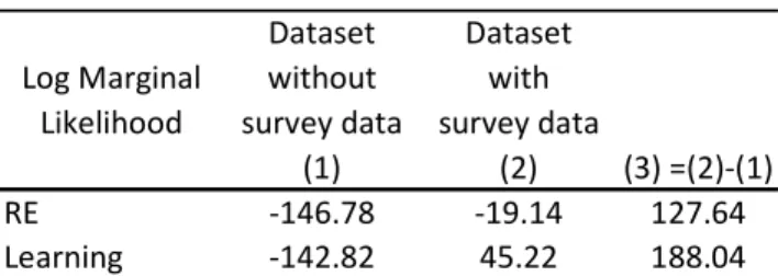
Table 2 shows the logarithm (log) of the marginal likelihoods of the RE and the learning solutions both when survey data are included in the estimation and when they are not. In the latter case, both solutions show similar log marginal likelihoods (see column 1). The log marginal likelihood difference of 3.96 points is not very robust (it goes down to less than 1
[
]
1 0, , 1 1, , 1 1, , 1
ˆ ˆt t t t t 1 ˆt
Eπ+ = − + π β π − +β π −π β π − π ′, which represents the row of Equation (4) that corresponds to
inflation expectations. If I add
π
to both sides of the equation and the measurement error on the RHS, I get Equation (8b).16
when choosing different priors)18; and thus, there is no clear evidence in favor of learning. However, this result changes significantly when survey data are included in the estimation (see column 2). Now learning clearly outperforms the RE solution, with a difference of 64.36 points in the log marginal likelihood, which implies a posterior odd of 8.93E+27 in favor of the former specification.
Table 2 Model comparison
Dataset Dataset
Log Marginal without with
Likelihood survey data survey data
(1) (2) (3) =(2)-(1)
RE -146.78 -19.14 127.64
Learning -142.82 45.22 188.04
Notes: This table shows the log marginal likelihood for RE and Learning. Survey data on inflation expectations come from the SPF one-quarter-ahead median forecast of the GDP deflator.
Does learning provide a better description of the survey data on inflation expectations than the RE assumption does? To answer this question, I follow Del Negro and Eusepi (2010) and calculate how well the model fits the series of inflation expectations conditional on the parameter distribution delivering the best possible fit for the rest of the macroeconomic indicators. The object of interest has the following representation:
1, 1, 1, 1, 1,
( eT T, i) ( eT , T, i) ( T, i) p dlP Y M =
∫
p dlPθ
Y M pθ
Y M dθ
,where Y1,T and dlP1,eT represent the series of macroeconomic indicators of Equation (7) and the survey data on inflation expectations, respectively, with observations going from 1 to T.
1, ( T, i)
p
θ
Y M represents the posterior distribution of the parameters of the model,θ
, which are obtained from the estimation of the model ignoring survey data. Finally, Mi corresponds to the solution of the model that could be obtained either under RE or learning.Column (3) of Table 2 shows the logarithm ofp dlP( 1,eT Y1,T,Mi), which is determined by the
difference between column (2), logarithm of p dlP( 1,eT,Y1,T Mi), and column (1), logarithm of
18
Using uniform prior distributions, I find log marginal likelihood values for the RE and learning specifications of -120 and -119.2, respectively. Moreover, Del Negro and Schorfheide (2008) shows that even 5 points in the log marginal likelihood can be overturned by choosing a slightly different prior.
17 1,
( T i)
p Y M . According to this measure, learning clearly outperforms RE in describing the evolution of the survey data. This result implies that the predictive power of the SW model can be improved by resorting to available survey data and to an admissible learning rule for the formation of expectations.19
Figure 3
Inflation expectations: survey data and model-implied expectations Database includes survey data
1970 1975 1980 1985 1990 1995 2000 2005 0 0.5 1 1.5 2 2.5 3 Survey data RE Learning
Notes: The model-implied inflation expectations are obtained using the Kalman-filtered estimates at each set of parameter values that conforms the posterior distributions. The grey and black areas represent the distance between the 5th and 95th percent confidence bands.
In addition, a graphical evaluation of the model-implied series of inflation expectations shows that learning improves the description of the evolution of survey expectations (see Figure 3). In particular, the RE solution under-predicts the survey expectations during the late 1970s and the early 1980s. It also over-predicts survey expectations at the beginning and end of the sample. However, the solution under learning is flexible enough to match more closely the fluctuations in the survey data, with a few exceptions.20 First, the model-implied inflation forecast over-predicts survey expectations in 1974:4. This result can be explained by the significant and sharp increase in inflation observed after the first oil crisis. Second, the
19 I would like to thank an anonymous referee for highlighting this point.
20 The better performance of learning in matching the survey data on inflation expectations can also be measured
by the correlation between surveys and the model-implied series of inflation expectations. When measured in levels, the correlation coefficients equal 0.870 and 0.938 for RE and learning, respectively. In first differences, the correlation coefficients for both cases are 0.201 and 0.276, respectively. These differences are statistically significant.
18
implied inflation forecast obtained under learning, but also under RE, under-predicts survey data in 1983. During both this year and the previous one, the important reduction in inflation was not accompanied by a similar-sized reduction in inflation expectations of the SPF. The closely related dynamics of inflation and inflation expectations in the RE solution and the high estimate of the perceived inflation persistence in the learning specification obtained for this time constitute the reasons why both specifications fail to track the evolution of survey data for this period.
4.3 Posterior estimates
The next step is to compare the posterior estimates obtained under RE and learning when survey data on inflation expectations are not employed in the estimation of the DSGE model (see Table 3). Taking the estimates of the RE solution as the benchmark case (column 1), the estimation under learning (column 2) results in a lower autocorrelation coefficient of the price mark-up shock, lower price stickiness, and higher price indexation. These results are compatible with Slobodyan and Wouters (2009b); however, they are not compatible with the results of Milani (2007). Milani (2007) finds that the introduction of learning forces the degree of habits in consumption and inflation indexation almost down to zero, while the autocorrelation coefficient of the supply shocks increases significantly (from a posterior mean of 0.02 in his rational expectations estimation (Table 3) to 0.854 in his benchmark learning estimation (Table 2)). As in Slobodyan and Wouters (2009b), I use small forecasting models for inflation while Milani uses forecasting models that are compatible with the RE solution of his model.21 Additionally, I employ external habits in consumption, unlike Milani, who employs internal habits. These differences may explain the discrepancies between our results and Milani’s.
When estimating both the RE and learning solutions using survey data on inflation expectations, I find that the most important changes in the parameter estimates are observed in the RE solution. In particular, I find that the price indexation significantly decreases (from a posterior median of 0.327 to 0.052), the autocorrelation coefficient of the price mark-up shocks increases (from a posterior median of 0.448 to 0.726), and the wage stickiness slightly decreases (from 0.554 to 0.468) (see Table 3, column 3). In the learning estimation, the only significant change in the parameter estimates is observed in the gain parameter for inflation,
21 I call a “small” forecasting model those models that use fewer regressors than the implied RE solution of the DSGE
19
which decreases from 0.188 to 0.141 (see Table 3, column 4).22 As a result, the additional moment restriction that represents the inclusion of the survey data on inflation expectations highlights the differences in the sources of inflation persistence. In the RE solution, inflation persistence depends on the persistence of the price mark-up shock. This occurs despite the fact that the model incorporates nominal frictions such as price stickiness and indexation. In contrast, under learning, both price indexation and the learning process itself are the main sources of the persistence of inflation.
Table 3
Posterior distribution statistics
Symbol Median Std Median Std Median Std Median Std
Wage stickiness ξw 0.554 0.045 0.547 0.049 0.468 0.043 0.563 0.049
Price stickiness ξp 0.648 0.044 0.481 0.035 0.629 0.058 0.480 0.035
Wage indexation ιw 0.482 0.131 0.314 0.107 0.442 0.124 0.319 0.107
Price indexation ιp 0.327 0.155 0.544 0.108 0.052 0.025 0.515 0.119
TR: inflation rπ 1.666 0.130 1.396 0.116 1.711 0.114 1.398 0.104
TR: lag interest rate ρR 0.760 0.028 0.763 0.028 0.706 0.030 0.777 0.029
TR: change in output rΔy 0.199 0.046 0.203 0.046 0.187 0.044 0.210 0.047
aut. Price Mk up shock ρp 0.448 0.195 0.140 0.070 0.726 0.078 0.173 0.087
std. Price mkup shock σp 0.145 0.026 0.213 0.017 0.112 0.013 0.204 0.014
gain - inflation gπ 0.188 0.014 0.141 0.009
gain - others gnonπ 0.031 0.042 0.019 0.031
Measurement exp error σexp 0.265 0.016 0.176 0.010
Log. Mg. Likelihood
(3) (4)
-142.8
WITH survey data WITHOUT survey data
RE Learning RE Learning
-19.1 45.2
-146.8
(1) (2)
Notes: this table shows the median and standard deviation of the posterior distributions of those parameters most closely related to the dynamics of inflation. The Online Appendix contains the same statistics for the complete list of parameters of the model, their prior and posterior distributions and a convergence check of the random walk Metropolist-Hasting.
Additionally, I would like to comment on the posterior median estimate obtained for the gain parameter for inflation because it is higher than the estimates reported by previous studies.23 For instance, Orphanides and Williams (2005a) consider a baseline calibrated value of the gain
22 The use of more data in the estimation of a DSGE model could eliminate the flat areas of the likelihood function
related to some parameters or combinations of them and, thus, may help to solve problems of weak identification (as discussed by Canova and Sala (2009)). However, in this study, I do not observe such improvements when incorporating survey data on inflation expectations into the estimation of the DSGE model (with the exceptions of the gain parameter for inflation in the learning specification and the standard deviation of the price mark-up shock under rational expectations).
23 Constant-gain parameter values of 0.188 and 0.141 imply that 75 percent of the information that people employ
to generate their inflation expectations is contained in the 6.7 and 9.1 most recent quarterly data observations, respectively. Because the relative weight of the j most recent observations in the estimation of the forecasting model is g(1-g)j-1, the number of observations required to accumulate the p percent of information used in this estimation is given by log(1-p)/log(1-g).
20
parameter of 0.02 and Milani (2007) and Slobodyan and Wouters (2009a) find posterior mean estimates that range between 0.0161 and 0.0247 and between 0.002 and 0.02, respectively. The high values for this parameter obtained in our study are related to the specification of the forecasting model. As the econometric exercise implemented in subsection 4.1 illustrates, the forecasting models for inflation that are the best fit for the survey data require significant time variation of their coefficients (the gain parameters are greater than or equal to 0.10). Moreover, the fewer variables that are included in the forecasting model, the smaller the impact of the time-variation of their coefficients on the stability of the DSGE model. Thus, not only does the forecasting model for inflation require high levels of time-variability in its coefficients, but it also allows me to estimate the DSGE model for these levels of time-variability. Finally, it is important to mention that Slobodyan and Wouters (2009b) also find a high degree of time-variability in the coefficients of the small forecasting models employed in their learning estimation. However, this result is not reflected in a high gain parameter because they use a Kalman-filter learning and not a constant-gain learning.
The reduction in the posterior mean of the gain parameter for inflation obtained using survey data to estimate the DSGE model has some interesting effects on the evolution of the coefficients of the forecasting model of inflation, the composition of inflation expectations, and the evolution of the inflation target implied by the model.
Figure 4
Evolution of the coefficients of the forecasting model for inflation (a) Perceived persistence of inflation (b) Intercept
1970 1975 1980 1985 1990 1995 2000 2005 -0.5
0 0.5 1
Without survey data With survey data
1970 1975 1980 1985 1990 1995 2000 2005 -0.2 0 0.2 0.4 0.6 0.8 1 1.2 1.4 1.6
Without survey data With survey data
As shown in Figure 4, when survey data are not included in the estimation, the perceived inflation persistence (
β
1,π) shows a sharp decline at the end of the 1970s with a subsequent increase. When survey data are included, the evolution of this coefficient does not exhibit this21
decline but remains high during the second half of the 1970s and throughout the 1980s. Additionally, the increases in the intercept of the forecasting model (
β
0,π) observed during the late 1970s and the early 1980s are less important.Figure 5
Composition of inflation expectations under learning (a) Not using survey data
1970 1975 1980 1985 1990 1995 2000 2005 -0.5 0 0.5 1 1.5 2 2.5 3 3.5 Inflation expectations Infl exp explained by intercept Infl exp explained by slope*inflation
(b) Using survey data
1970 1975 1980 1985 1990 1995 2000 2005 -0.5 0 0.5 1 1.5 2 2.5 3 3.5 Inflation expectations Infl exp explained by intercept Infl exp explained by slope*inflation
These differences in the evolution of the coefficients of the forecasting model affect the composition of inflation expectations. The form of the forecasting model lead conditional inflation expectations to be represented as E dlPt( t+1)=
β
0, ,πt+β
1, ,πtdlPt. When survey data are included in the estimation, it becomes evident that up to the beginning of the 1990s, these expectations were closely related to the evolution of the perceived persistence of inflation,22 1, ,tπ dlPt
β
(see Figure 5b). However, this is not the case when survey data are absent (Figure 5a). In addition, since the 1990s, both estimations indicate that inflation expectations are no longer related to the perceived persistence of inflation but to the perceived inflation mean.24Finally, Figure 6 shows the evolution of the perceived long-run inflation target at each point in time, which can be expressed by
β
0,π (1−β
1,π). According to this figure, at the beginning of the 1970s the expected quarterly inflation target was 0.59 percent, but it kept increasing until it reached 2.44 percent in 1981:2. Afterwards, I observe an important reduction down to a level between 0.6 and 1 during the 1980s. The timing and the magnitude of the reduction in expected inflation target are consistent with the belief that the Volcker recession at the beginning of the 1980s reduced inflation expectations. During the 1990s, the target steadily decreased until the early 2000s (in 2000:1, the target was 0.37). After this point, the expected inflation target follows a positive path that was interrupted by the outbreak of the financial crisis in 2007. The use of survey data in the estimation avoids the influence of some outliers observed in the evolution of the inflation target.Figure 6
Evolution of the inflation target under learning
1970 1975 1980 1985 1990 1995 2000 2005 -1 -0.5 0 0.5 1 1.5 2 2.5 3
Without survey data With survey data
24 Given the structure of the forecasting model for inflation, if the perceived persistence coefficient is close to zero,
23
4.4 Impulse-Response analysis
Finally, I analyze how the use of survey data affects the Impulse-Response functions (IRFs) analysis for inflation. I only focus on this variable because the introduction of survey data does not affect the IRFs for the other variables of the model.25
Under the RE solution, there is only a significant difference in the IRFs obtained when survey data are used in the estimation of the DSGE model and when they are not. This case is the response of inflation to the wage mark-up shock. The reduction of the wage stickiness obtained when survey data are used results in a less persistent inflation response to the wage mark-up shock (see Figure 7a). Interestingly, despite the large reduction in the degree of inflation indexation, the impact of a price mark-up shock on inflation is not significantly altered with the use of survey data (see Figure 7b). The underlying reason is the compensation of the declining price indexation by the increasing autocorrelation coefficient of the price mark-up shock.
Figure 7
IRFs under RE: response of inflation to price and wage mark-up shocks
(a) Wage mark-up shock (b) Price mark-up shock
-0.05 0 0.05 0.1 0.15 0.2 0.25 1 2 3 4 5 6 7 8 9 10 11 12 13 14 15
Without survey data With survey data
-0.1 -0.05 0 0.05 0.1 0.15 0.2 0.25 0.3 0.35 1 2 3 4 5 6 7 8 9 10 11 12 13 14 15
Without survey data With survey data
Notes: This figure shows the responses of inflation to a price and a wage mark-up shocks. Dotted lines are the 90% confidence intervals.
Under learning, adding survey data leads to a reduction in the time-variability of the coefficients of the forecasting model for inflation, thus reducing the time-variability of the IRFs. As a result, most of the stronger and more persistent responses of inflation are concentrated in the 1970s. For instance, it is observed that unexpected monetary policy shocks had a stronger destabilizing effect on inflation during the 1970s than afterwards (see Figure 8).
25 The Online Appendix contains the variance-covariance analysis for inflation. I find that the relative importance of
24
This result is compatible with the study by Boivin and Giannoni (2006), who found weaker responses of inflation to unexpected changes in the interest rate during the post-1979 period than during the pre-1979 period. When survey data are excluded from the estimation of the DSGE model, the higher time-variability of the coefficients of the forecasting model for inflation produce important responses of inflation to structural shocks during the 1990s and 2000s, that otherwise would have not being observed.
5. Robustness exercises
In order to test my findings for robustness, I evaluate the following three variations of our benchmark specification. First, I use alternative specifications of the forecasting model for inflation under learning. Second, I analyze how our results change when we use loose uniform priors.26 Finally, I replace the CG-LS algorithm used under learning with ordinary least squares (OLS).
Table 4
Posterior distribution statistics: different specifications of the forecasting model for inflation Estimations include survey data on inflation expectations
Symbol Median Std Median Std Median Std Median Std Median Std
Wage stickiness ξw 0.563 0.049 0.555 0.048 0.548 0.046 0.548 0.046 0.551 0.048
Price stickiness ξp 0.480 0.035 0.446 0.033 0.467 0.037 0.453 0.035 0.462 0.037
Wage indexation ιw 0.319 0.107 0.314 0.101 0.342 0.110 0.326 0.106 0.319 0.109
Price indexation ιp 0.515 0.119 0.584 0.118 0.553 0.118 0.618 0.112 0.674 0.101
TR: inflation rπ 1.398 0.104 1.432 0.111 1.404 0.121 1.468 0.111 1.423 0.115
TR: lag interest rate ρR 0.777 0.029 0.775 0.029 0.767 0.029 0.778 0.023 0.776 0.031
TR: change in output rΔy 0.210 0.047 0.210 0.045 0.203 0.046 0.214 0.044 0.206 0.046
aut. Price Mk up shock ρp 0.173 0.087 0.180 0.083 0.168 0.083 0.175 0.080 0.124 0.062
std. Price mkup shock σp 0.204 0.014 0.221 0.014 0.206 0.015 0.223 0.013 0.221 0.014
gain - inflation gπ 0.141 0.009 0.132 0.006 0.137 0.007 0.130 0.005 0.140 0.008
gain - others gnonπ 0.019 0.031 0.023 0.022 0.028 0.049 0.019 0.021 0.019 0.032
Measurement exp error σexp 0.176 0.010 0.177 0.011 0.175 0.009 0.173 0.009 0.184 0.011
Log. Mg. Likelihood (1) dlP (benchmark) 45.2 38.6 43.3 40.4 (5) dlP dlGDP 24.1 lHours dlP lHours (2) (3) (4) dlP dlCons dlP dlCons
Notes: this table shows the median and standard deviation of the posterior distributions of those parameters most closely related to the dynamics of inflation. Each of the columns indicates the use of different specifications of forecasting models for inflation. These specifications are the ones that generate the series of one-period-ahead inflation forecasts closer to the series of survey data on inflation expectations.
When using alternative forecasting models for inflation, the posterior statistics obtained under learning barely change (see Table 4, columns 2 to 5).27 In particular, the median values of the posterior distribution of the price indexation and the autocorrelation coefficient of the price
26 The Online Appendix contains the list of prior distributions used for these estimations. 27
25 Figure 8
IRFs under learning: Response of inflation to wage mark-up, productivity and monetary policy shocks
Without using survey data Using survey data
(a) Wage mark-up shock
1969Q1 1974Q1 1979Q1 1984Q1 1989Q1 1994Q1 1999Q1 2004Q1 0 10 20 -0.3 -0.2 -0.1 0 0.1 0.2 0.3 0.4 1969Q1 1974Q1 1979Q1 1984Q1 1989Q1 1994Q1 1999Q1 2004Q1 0 10 20 -0.3 -0.2 -0.1 0 0.1 0.2 0.3 0.4 (b) Productivity shock 1969Q1 1974Q1 1979Q1 1984Q1 1989Q1 1994Q1 1999Q1 2004Q1 0 10 20 -0.2 -0.15 -0.1 -0.05 0 0.05 0.1 0.15 1969Q1 1974Q1 1979Q1 1984Q1 1989Q1 1994Q1 1999Q1 2004Q1 0 10 20 -0.2 -0.15 -0.10 -0.05 0 0.05 0.1 0.15
(c) Monetary policy shock
1969Q1 1974Q1 1979Q1 1984Q1 1989Q1 1994Q1 1999Q1 2004Q1 0 10 20 -0.2 -0.15 -0.1 -0.05 0 0.05 0.1 0.15 1969Q1 1974Q1 1979Q1 1984Q1 1989Q1 1994Q1 1999Q1 2004Q1 0 10 20 -0.2 -0.15 -0.1 -0.05 0 0.05 0.1 0.15
Notes: This figure shows the responses of inflation to a wage mark-up, productivity and monetary policy shocks using the structure of the economy at every point in time.
26
mark-up shock are close to 0.60 and 0.161, respectively, and the gain parameter for inflation is close to 0.135. These numbers are very similar to those obtained under the benchmark specification of the forecasting model for inflation (column 1).
With respect to the introduction of loose uniform prior distributions, I find that learning does not display a major change in most of the parameter estimates, with the exception being the increases in wage stickiness and the Taylor rule’s coefficient of output growth (for details, please refer to the Online Appendix). The latter result is also observed under RE.
Finally, the use of the OLS algorithm instead of CG-LS significantly decreases the log marginal likelihood of learning when survey data are included (Table 5, column 2). This result can be explained by the inability of this specification to match the evolution of the survey data. The OLS algorithm keeps the coefficients of the forecasting model very close to the initial conditions. Given that the initial conditions are obtained during a period of low and not persistent inflation (period 1950:1-1968:3), the model fails to replicate the increases in the expectations during the 1970s and beginning of the 1980s (see the Online Appendix). Yet, the RE solution also fails to match the evolution of the survey data in the same way as learning does when the CG-LS is employed.
Table 5
Model comparison: estimation using OLS learning Dataset Dataset
Log Marginal without with
Likelihood survey data survey data
(1) (2) (3)=(2)-(1)
RE -146.78 -19.14 127.64
Learning -148.35 -77.20 71.14
Notes: This table shows the log marginal likelihood for RE and Learning. Survey data on inflation expectations come from the SPF one-quarter-ahead median forecast of the GDP deflator.
6. Conclusions
In this paper, I provide evidence that the predictive power of DSGE models is improved when using available survey data and an admissible learning rule for the formation of expectations. In particular, I find that the solution under learning of the New Keynesian model developed by
27
SW fits the data better than the RE solution once survey data on inflation expectations are included in the analysis.
Moreover, I employ survey data on inflation expectations in selecting the forecasting model for inflation under learning, thus reducing, to some extent, the degree of freedom the researcher faces at the time of choosing the forecasting models. The resulting small forecasting model for inflation and the high speed of learning allow the SW model, when solved under learning, to match the increases and decreases in inflation expectations observed during the late 1970s and the early 1980s.
Finally, the additional moment restriction that represents the inclusion of the survey data on inflation expectations leads to parameter estimates that highlight the differences in the sources of inflation persistence between RE and learning. Under RE, a highly persistent price mark-up shock is observed, despite the fact that this model incorporates nominal frictions such as price stickiness and indexation. In contrast, both price indexation and the learning process itself are the main sources of inflation persistence under learning.
Several important issues are not addressed in this study. First, I only use the median value of inflation expectations reported by the forecasters included in the SPF at each point in time. However, it is possible to exploit information about other moments – such as the dispersion – to evaluate issues like the credibility of the central bank or the effect of periods of high disagreement in expectations on the conduct of monetary policy. Second, survey data on inflation expectations may be employed to evaluate models particularly designed to better explain the low-frequency movements of inflation observed during the late the 1970s and the early 1980s in many developed countries. In light of our results, it is interesting to ask whether other perfect information setups (such as those in Sbordone (2007) or Ireland (2007)) can provide better descriptions of the survey data than learning can. Finally, survey data are also available for a variety of other macroeconomic indicators besides inflation expectations. For instance, survey data on expectations of future output and investment growth might contain useful information for the identification of the mechanisms underlying the business cycle. To conclude, this study is one of the first to show that survey data contain useful information for estimating DSGE models. Yet, empirical macroeconomic studies have been largely neglected the information collected by surveys such as the SPF, the Livingstone and University of Michigan surveys and the Greenbook. The use of this information could improve our understanding of how expectations are formed and their impact on the economy.