Scalable Inference in Latent
Gaussian Process Models
DISSERTATION
zur Erlangung des akademischen Grades
doctor rerum naturalium
(Dr. rer. nat.)
im Fach Informatik
eingereicht an der
Mathematisch-Naturwissenschaftlichen Fakult¨
at
der Humboldt-Universit¨
at zu Berlin
von
M.Sc. Florian Wenzel
Pr¨
asidentin der Humboldt-Universit¨
at zu Berlin:
Prof. Dr.-Ing. Dr. Sabine Kunst
Dekan der Mathematisch-Naturwissenschaftlichen Fakult¨
at:
Prof. Dr. Elmar Kulke
Gutachter/innen:
1. Prof. Dr. Marius Kloft
2. Prof. Dr. Manfred Opper
3. Prof. Dr. Stephan Mandt
Abstract
Latent Gaussian process (GP) models help scientists to uncover hidden structure in data, express domain knowledge and form predictions about the future. These models have been successfully applied in many domains including robotics, geology, genetics and medicine. A GP defines a distri-bution over functions and can be used as a flexible building block to de-velop expressive probabilistic models. The main computational challenge of these models is to make inference about the unobserved latent random variables, that is, computing the posterior distribution given the data. Currently, most interesting Gaussian process models have limited appli-cability to big data. Naive inference typically scales cubically in the num-ber of data points and exact computation of posterior is intractable and requires approximations like variational inference. Recent work around so-called sparse Gaussian process techniques has enabled the application of several GP models to big datasets. However, these methods are often unstable and inefficient since they are based on numerical approximations of the gradients of the variational objective.
This thesis develops a new efficient inference approach for latent GP mod-els. Our new inference framework, which we call augmented variational inference, is based on the idea of considering an augmented version of the intractable GP model that renders the model conditionally conjugate. We show that inference in the augmented model is more efficient and, unlike in previous approaches, all updates can be computed in closed form. The ideas around our inference framework facilitate novel latent GP mod-els that lead to new results in language modeling, genetic association stud-ies and uncertainty quantification in classification tasks. We develop new inference methods for binaryGP classification,multi-class GP classifica-tionand theBayesian support vector machine, which are up to two orders of magnitude faster than the state of the art. Furthermore, we propose two novel latent GP models. Thesparse GP linear mixed modelconcerns feature selection in confounded data with binary labels and the general-ized dynamic topic model can be used to analyze massive collections of text data by exploring topics that evolve over time.
Zusammenfassung
Latente Gauß-Prozess-Modelle (latent Gaussian process models) werden von Wissenschaftlern benutzt, um verborgenen Muster in Daten zu er-kennen, Expertenwissen in probabilistische Modelle einfließen zu lassen und um Vorhersagen ¨uber die Zukunft zu treffen. Diese Modelle wur-den erfolgreich in vielen Gebieten wie Robotik, Geologie, Genetik und Medizin angewendet. Gauß-Prozesse definieren Verteilungen ¨uber Funk-tionen und k¨onnen als flexible Bausteine verwendet werden, um aussa-gekr¨aftige probabilistische Modelle zu entwickeln. Dabei ist die gr¨oßte Herausforderung, eine geeignete Inferenzmethode zu implementieren. In-ferenz in probabilistischen Modellen bedeutet die A-Posteriori-Verteilung der latenten Variablen, gegeben der Daten, zu berechnen. Die meisten interessanten latenten Gauß-Prozess-Modelle haben zurzeit nur begrenz-te Anwendungsm¨oglichkeiten auf großen Datens¨atzen. Naive Inferenzme-thoden skalieren kubisch in der Anzahl der Datenpunkte und die exak-te Berechnung der A-Posexak-teriori-Verexak-teilung ist nicht m¨oglich und bedarf approximativer Methoden wie variational inference. Neue wissenschaftli-che Ver¨offentlichungen um sogenannte sparse Gaussian processes haben es erm¨oglicht, dass einige Gauß-Prozess-Modelle auf großen Datenmengen angewendet werden k¨onnen. Trotzdem sind diese Methoden oft instabil und ineffizient, da sie auf numerischen Approximationen des Gradienten der variationellen Zielfunktion beruhen.
In dieser Doktorarbeit stellen wir eine neue effiziente Inferenzmethode f¨ur latente Gauß-Prozess-Modelle vor. Unser neuer Ansatz, den wir aug-mented variational inference nennen, basiert auf der Idee, eine erweiterte (augmented) Version des Gauß-Prozess-Modells zu betrachten, welche be-dingt konjugiert (conditionally conjugate) ist. Wir zeigen, dass Inferenz in dem erweiterten Modell effektiver ist und dass alle Schritte des va-riational inference Algorithmus in geschlossener Form berechnet werden k¨onnen, was mit fr¨uheren Ans¨atzen nicht m¨oglich war.
Unser neues Inferenzkonzept erm¨oglicht es, neue latente Gauß-Prozess-Modelle zu studieren, die zu innovativen Ergebnissen im Bereich der Sprach-modellierung, genetischen Assoziationsstudien und Quantifizierung der
Unsicherheit in Klassifikationsproblemen f¨uhren. In der vorliegenden Ar-beit entwickeln wir neue Inferenzmethoden f¨ur binary Gaussian process classification,multi-class GP classification und die Bayesian support vec-tor machine. Unsere Methode ist bis zu zwei Gr¨oßenordnungen schneller als vorherige Methoden. Dar¨uber hinaus entwickeln wir zwei neue latente Gauß-Prozess-Modelle. Das sparse Gaussian process linear mixed model
kann f¨ur die Merkmalserkennung (feature selection) in Daten mit bin¨aren Labels verwendet werden und kann mit confounding Effekten umgehen. Mit dem generalized dynamic topic model k¨onnen große Textdatens¨atze analysiert werden und Themen im Text gefunden werden, die sich ¨uber die Zeit ver¨andern.
Acknowledgements
First of all, I would like to thank my PhD advisor, Prof. Marius Kloft, for his advice and encouragement. Marius gave me much freedom in following my research interests and supported me in every way to travel and collaborate with other researchers.
I am very grateful to Prof. Stephan Mandt for kindly inviting me to visit his group at Disney Research in Pittsburgh. We continued to collaborate on many projects and I always greatly enjoyed our countless stimulating discussions.
I want to express my sincere gratitude to Prof. Manfred Opper. I spend one and a half year as a visiting researcher in his lab. I was always in-trigued by his wisdom and his great knowledge of old papers and “Physi-cists tricks” that often lead to new fascinating ideas.
My special thanks go to Th´eo Galy-Fajou with whom I shared an office for two years. We worked on many projects together and I always enjoyed Th´eo’s enthusiasm for discussing new ideas and creating neat visualiza-tions (especially animavisualiza-tions) of our results.
I am grateful to the Machine Learning Group at Humboldt-Universit¨at zu Berlin, the Machine Learning Group at TU Kaiserslautern and the Group of Artificial Intelligence at TU Berlin—especially Andreas, Burak, Christian, Cordula, Dimitra, Heike, Ludovica, Matth¨aus, Patrick, Robert for many engaging discussions. I also want to thank Nadia Sakhi and Dr. Robert Bamler for their valuable feedback on the manuscript.
Most of all, I would like to thank Ronja and my parents for supporting me in every conceivable way.
Finally, I acknowledge financial support of the German Bundesminis-terium f¨ur Bildung und Forschung (BMBF) under the awards 01IS18051A and 031B0187B, and the German Research Foundation (DFG) under the award KL 2698/2-1.
Contents
Basic notation xi
I
Overview
1
1 Introduction 2
1.1 Organization and contributions . . . 5
1.2 Brief introduction to Gaussian process models . . . 7
2 Augmented Variational Inference for Gaussian Process Models 13 2.1 A conditionally conjugate formulation via auxiliary variable augmen-tation . . . 14
2.2 Variational inference in the augmented model . . . 15
2.3 On the quality of the augmented approximation . . . 16
2.4 Gibbs sampling . . . 18
II
Scalable Inference in Latent Gaussian Process Models 20
3 Gaussian Process Classification 21 3.1 Background and related work . . . 223.2 The augmentation . . . 23
3.3 Inference . . . 25
3.4 Experiments . . . 27
3.4.1 Quality of the approximation . . . 28
3.4.2 Numerical comparison . . . 28
4 Multi-class Gaussian Process Classification 34
4.1 Background and related work . . . 36
4.2 Conjugate multi-class Gaussian process classification . . . 38
4.2.1 The logistic-softmax GP model . . . 38
4.2.2 Towards a conjugate augmentation . . . 39
4.3 Inference . . . 41
4.3.1 Variational approximation . . . 42
4.3.2 Inference method . . . 42
4.4 Experiments . . . 45
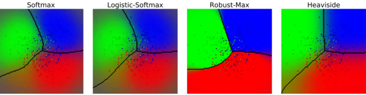
4.4.1 Comparison of the different likelihoods . . . 46
4.4.2 Effect of the augmentation . . . 48
4.4.3 Inducing points and hyperparameters . . . 50
4.4.4 Numerical comparison . . . 50
5 Bayesian Support Vector Machine 53 5.1 Background and related work . . . 55
5.2 The augmentation . . . 56
5.3 Inference . . . 57
5.4 Experiments . . . 60
5.4.1 Prediction performance and uncertainty estimation . . . 60
5.4.2 Big data experiment . . . 61
5.4.3 Auto tuning of hyperparameters . . . 62
5.4.4 Inducing points selection . . . 63
6 Sparse Gaussian Process Linear Mixed Model: Feature Extraction in Confounded Data 65 6.1 Sparse Gaussian process linear mixed model . . . 67
6.2 Background and related work . . . 69
6.3 Inference . . . 70
6.4 Inference via expectation propagation . . . 71
6.5 Inference via augmented variational inference . . . 76
6.6 Experiments . . . 80
6.6.1 General experimental setup . . . 81
6.6.2 Simulated data . . . 82
6.6.3 Tuberculosis disease outcome prediction . . . 84
6.6.4 Malicious computer software (malware) detection . . . 87 6.6.5 Flowering time prediction from single nucleotide polymorphisms 88
6.6.6 Big data experiment . . . 89
7 Generalized Dynamic Topic Models 91 7.1 Background and related work . . . 93
7.2 Generalized dynamic topic models . . . 94
7.2.1 Generalized DTMs . . . 94
7.2.2 A side note on augmenting the model . . . 96
7.3 Inference . . . 97
7.4 Experiments . . . 100
8 Conclusions and Outlook 107 Appendix 110 A Gaussian process classification 110 A.1 Variational bound . . . 110
A.2 Variational updates . . . 112
A.3 Variational bound by Gibbs and MacKay . . . 113
A.4 Additional performance plots . . . 114
B Multi-class Gaussian process classification 118 B.1 Reparametrization of the P´olya-Gamma variables . . . 118
B.2 Subsampling the classes (extreme classification version) . . . 119
C Bayesian support vector machine 120 C.1 Derivation of the variational objective . . . 120
C.2 Euclidean and natural gradients of the variational objective . . . 122
C.3 Optimization of the kernel hyperparameters . . . 124
D Sparse Gaussian process linear mixed model 125 D.1 Convexity of the Objective Function . . . 125
D.2 Gradient and Hessian . . . 125
E Generalized dynamic topic models 128 E.1 Derivation of the variational objective . . . 128
E.2 SVI updates . . . 129
E.3 Global td-idf score . . . 131
Basic notation
Unbolded x represents a single number, boldface x represents a vector, and capital unbolded X represents a matrix. An individual element of a vector is denoted with a subscript and without boldface. For example, the i-th element of a vector x is xi. A bold lower-case letter with an index such as xj represents a particular row of a matrix X (e.g. a data pointxj of the data matrix X).
Symbol Description
f A function f :Rd→
R.
f A vector of function values, whosei-th element is given byf(xi), where xi is thei-th data point.
Yi. The i-th row of a matrix Y. Y.j The j-th column of a matrix Y.
Knn Shorthand for the kernel matrix of the training points.
Knm Shorthand for the kernel matrix between the training and in-ducing points.
Kmm Shorthand for the kernel matrix between the inducing points. KL(.||.) Kullback-Leibler divergence.
L Evidence lower bound (ELBO).
B(.|p) Bernoulli distribution with parameter p. Cat(.|p) Categorical distribution with parameter p.
Dir(.|α) Dirichlet distribution with concentration parameter α.
Ga(.|a, b) Gamma distribution with shape parameteraand rate parameter b.
GIG(.|a, b, c) Generalized inverse Gaussian distribution with parameters a, b, c.
N(.|µ,Σ) Gaussian distribution with mean parameter µ and covariance matrix Σ.
PG(.|a, b, c) P´olya-Gamma distribution with parameters a, b, c. Po(.|λ) Poison distribution with rate parameter λ.
Part I
Overview
Chapter 1
Introduction
Gaussian processes (GPs) (Rasmussen and Williams, 2006) provide a popular Bayesian non-parametric framework, which can be used to address challenging machine learning problems. Because of their ability of accurately adapting to data and thus achieving high prediction accuracy while providing well calibrated uncertainty estimates, GPs are a standard method in several application areas including robotics (Sæmundsson, Hofmann, and Deisenroth, 2018; Beckers, Kuli´c, and Hirche, 2019), facial behavior analysis (Eleftheriadis et al., 2017), electrical engineering (Shepero et al., 2018; Pan-dit and Infield, 2018) and geospatial predictive modeling where they are known as
kriging (Stein, 2012; Park and Apley, 2018).
Although deep learning has attracted tremendous attention from researchers in various fields such as language processing and computer vision, standard deep learn-ing systems lack the ability to represent uncertainty in a mathematically sound way (Ghahramani, 2015). This is a critical shortcoming since in many applications ar-eas including the life sciences as discussed by Herzog and Ostwald, 2013; Nuzzo, 2014, in biology and physics (Krzywinski and Altman, 2013), and self-driving cars (Michel-more, Kwiatkowska, and Gal, 2018), uncertainty information is crucial. In all these fields, we need systems that “know when they don’t know”.
Gaussian processes, on the other hand, provide a mathematically sound approach to uncertainty representation. GPs are useful for representing random latent functions in probabilistic models. Computing the posterior distribution, i.e. the distribution of the latent function given the observed data, leads to sensible uncertainty estimates in the predictions for new data points (Rasmussen and Williams, 2006).
Because of providing well calibrated uncertainty estimates, GPs inspired and are widely used in many modern Bayesian deep learning approaches including deep kernel learning (Wilson et al., 2016), deep Gaussian processes (Damianou and Lawrence, 2013) and in the analysis of Bayesian neural networks (G. Matthews et al., 2018;
θ τ β2 1 β1 1 βK 1 … β1 W β2 W βK W … … … … z w β y X f fi X σ( . ) … y f1 f2 fC X y f y X f θ τ β2 1 β1 1 βK 1 … β1 W β2 W βK W … … … … z w β y X f fi X σ( . ) … y f1 f2 fC X y f y X f θ τ β2 1 β1 1 βK 1 … βW1 βW2 βK W … … … … z w β y X f fi X σ( . ) … y f1 f2 fC X y f y X f θ τ β2 1 β1 1 βK 1 … β1 W β2 W βK W … … … … z w β y X f fi X σ( . ) … y f1 f2 fC X y f y X f θ τ β2 1 β1 1 βK 1 … βW1 β2 W βK W … … … … z w β y X f fi X σ( . ) … y f1 f2 fC X y f y X f y X f z Generalized DTM (Chapter 7)
GP Classification (Chapter 3) Bayesian SVM (Chapter 5)
Multi-class GP Classification (Chapter 4) Sparse GP LMM (Chapter 6)
Latent Gaussian Process Models
Latent Gaussian process Additional random variables Intermediate values Data
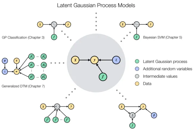
Figure 1.1: Latent Gaussian process models are probabilistic models that include one ore multiple latent GPs (green circles) and optionally additional latent random variables (blue circles), which are connected to the data (orange circles) via a possibly non-conjugate likelihood. In this thesis, we consider latent GP models of the structure as displayed in the center of the figure and develop an efficient inference approach for these models. Furthermore, we study five different models that are successfully applied in domains including binary and multi-class classification, genetic association studies and language modeling. All models can be cast as a latent GP model of the displayed structure and are amenable for our novel efficient inference approach. Jacot, Gabriel, and Hongler, 2018). Moreover, GPs influenced other new interesting approaches to probabilistic function approximation in deep learning systems including neural processes (Garnelo et al., 2018) and variational implicit processes (Ma, Li, and Hernandez-Lobato, 2019).
But what is a Gaussian process? A GP defines a distribution over functions and is characterized by the property that any finite set of function values f(x1), . . . , f(xN)
has a joint multivariate Gaussian distribution (Rasmussen and Williams, 2006). A GP is fully specified by its mean and covariance function, also called thekernel function. There are many possible choices of kernel functions, which give rise to a wide range of
different models. For instance, a GP based on the so-calledsquared exponential kernel
function leads to a distribution over smooth functions, and using alinear kernel leads to a distribution over linear functions. GPs are well suited for developing interesting models. They can be utilized as a flexible building block in probabilistic modeling and become more expressive as the number of training examples increases. Through the choice of the kernel function, we can incorporate prior knowledge into the model and express a wide range of modeling assumptions.
For example, let us consider the problem of supervised binary classification. In this setting, the task is to predict the class label y associated to a new data point x given some observed data D = {(x1, y1), . . . ,(xn, yn)}. This task can be modeled by assuming a non-linear latent function f(x), defined on the space of data points, that is connected to a corresponding class label y by a suitable likelihood function
p(y|f, x). We obtain a latent GP model by imposing a GP prior distribution over the latent function p(f).
By connecting latent Gaussian processes with suitable likelihood functions, we can build a wide range of different models. In this thesis, we study several novel latent Gaussian process models, which are successfully applied in domains including binary and multi-class classification, genetic association studies and language modeling. As displayed in Fig.1.1, all models discussed in this thesis can be framed as latent GP models.
To predict new data, we have to make inference about the latent GP(s). This is a challenging problem and the main concern of this thesis. Recent trends in data availability in the sciences and technology have made it necessary to develop algo-rithms capable of processing massive data (John Walker, 2014). Despite the above mentioned advantages, currently, GP models have limited applicability to big data. Naive inference typically scales cubically in the number of data points, and exact computation of posterior and marginal likelihood is intractable.
Nevertheless, the combination of so-called sparse Gaussian process techniques with approximate inference methods, such as expectation propagation (EP) or the variational approach, have enabled certain GP models, e.g. GP classification, to datasets containing millions of data points (Hensman and Matthews, 2015; Dezfouli and Bonilla, 2015; Hern´andez-Lobato and Hern´andez-Lobato, 2016; Salimbeni, Eleft-heriadis, and Hensman, 2018).
While these results are already impressive, we will show in this thesis that a speed-up of speed-up to two orders of magnitude can be achieved. We develop a novel scalable
variational inference approach for latent GP models, which builds on an auxiliary vari-able augmentation of the model. An auxiliary varivari-able is an additional latent varivari-able that is added to a model such that the original model is recovered when this variable is integrated out. In our approach, the main idea is to consider an augmented version of the GP model that renders the model conditionally conjugate. In a conditionally conjugate model, all complete conditional distributions (the posterior distribution of one random variable given all the others), can be computed in closed form. Moreover, we show that inference in the augmented conditionally conjugate model is much easier than in the original model and demonstrate superior performance over the state of the art.
1.1
Organization and contributions
The main contribution of this thesis is to develop a new efficient variational inference approach based on auxiliary variable augmentation. This thesis also contributes novel latent GP models that lead to new results in language modeling, genetic association studies and uncertainty quantification in classification tasks.
Part I: Introduction and Overview
I start my dissertation in Chapter 1 with a short introduction to latent GP models. I lay out the basic inference problem and present the concept of sparse GP approxi-mations.
In Chapter 2, I present a unifying view on a new efficient inference approach for latent GP models. The approach is called augmented variational inference and builds on an auxiliary variable augmentation technique. The main idea is to consider an augmented version of the latent GP model that renders the model conditionally conjugate. In the augmented model, we can derive an efficient variational inference algorithm, which is based on closed-form block coordinate ascent updates. These updates can be interpreted as natural gradient updates and are more efficient than ordinary Euclidean gradient updates. Additionally, the conditionally conjugate form of the model directly leads to an exact Gibbs sampling scheme.
Part II: Scalable Inference in Latent Gaussian Process Models
In the second part of my dissertation, I present five latent Gaussian process models. For each model, I develop a scalable inference method based on the principles laid out in the first part of the thesis and demonstrate superior performance over the state of
the art. Each chapter covers one model and can be read independently from the other chapters. For the sake of readability without interruptions, I briefly repeat the main concepts in each chapter while the details for the common ideas behind theaugmented variational inferenceapproach can be found in Chapter 2. The presented models and inference procedures are based on previous publications, which are indicated at the beginning of each chapter.
Chapter 3 considers Gaussian process classification based on the logistic likeli-hood function. I develop a stochastic variational inference method based on a P´ olya-Gamma augmentation of the likelihood. Unlike in previous work, all updates are given in closed form and do not rely on numerical quadrature methods or sampling. In the experiments, I demonstrate that theaugmented variational inference approach drastically improves computation time by up to two orders of magnitude while being competitive in terms of prediction performance.
Chapter 4 concerns multi-class GP classification. The multi-class classification problem is more complicated than the binary classification setting discussed in the previous chapter because it involves not only one latent GP, but one GP for each class. I introduce a novel multi-class GP classification model building on a modification of the softmax likelihood function. The new likelihood function has two advantages. First, it allows for an efficient auxiliary variable augmentation approach that renders the model conditionally conjugate. Second, it solves the calibration issue of previ-ous work on scalable multi-class GP classification as it leads to better uncertainty quantification.
In Chapter 5, I develop a scalable inference method for a Bayesian version of the support vector machine (SVM). Advantages of the Bayesian approach over the common standard version of the SVM include automatic treatment of hyperparam-eters and direct quantification of the uncertainty of the prediction, which can be of great importance in practice. The inference method is based on a generalized inverse Gaussian augmentation and the experiments demonstrate superior performance over competing methods in terms of uncertainty quantification and speed.
Chapter 6 concerns feature selection in confounded data. This is an important problem in genetic association studies. The goal of this field is to find causal as-sociations between high-dimensional vectors of genotypes, such as single nucleotide polymorphisms, and observable outcomes (feature selection). Genetic associations can be spurious, unreliable, and unreproducible when the data are subject to spu-rious correlations due to confounding. I propose the sparse Gaussian process linear mixed model, which finds relevant features while correcting for confounding. I discuss
two inference methods for two versions of the model. The first inference method is based on expectation propagation and is limited to small datasets. The second infer-ence method builds on anaugmented variational inferenceapproach and scales to big datasets, but introduces a slight additional approximation error. The scalable aug-mented variational inferencemethod was designed by me and implemented with the help of Lorenz Vaitl. In an experimental study on genetic data, I show that my new approach beats several baselines in terms of prediction performance, feature selection stability and finds features that are less correlated with the confounder.
In Chapter 7, I develop a new time dynamic topic model (DTM), which can be used for analyzing text data. DTMs model the evolution of prevalent themes in literature, online media and other forms of text over time. In the newgeneralized dynamic topic model, the time dynamics are governed by GPs. This allows for exploring topics that develop smoothly over time, that have a long-term memory or are temporally concentrated (for event detection). I discuss how to perform scalable approximate inference in this model. The experiments on several large-scale datasets show that my generalized model allows to find interesting patterns that were not accessible by previous approaches.
In Chapter 8, I conclude and discuss future work.
1.2
Brief introduction to Gaussian process models
In this section, we introduce the problem of learning from data via latent GP models. A GP defines a distribution over functionsf ∼GP(µ, k), whereµis the mean function and k is the kernel function. A GP is characterized by the property that any finite set of function valuesf(x1), . . . , f(xN) has a joint multivariate Gaussian distribution
(Rasmussen and Williams, 2006). The distribution is completely specified by the mean function
E[f(x)] =µ(x)
and the kernel function (also called covariance function) Cov[f(x), f(x0)] = k(x,x0).
In practice, we usually assume that the mean function is simply zero since uncertainty about the mean function can be taken into account by adding an extra term to the kernel (Rasmussen and Williams, 2006).
Each kernel function corresponds to a different set of assumptions we make about the function we wish to model (Rasmussen and Williams, 2006; Duvenaud, 2014). In particular, the type of kernel function determines the type of latent functions we expect to see and determines how the model generalizes to new data. There are many possible choices of kernel functions. For instance, the squared exponential kernel is defined by k(x,x0) =σf2exp −(x−x 0 )2 2`2 ! , where the variance parameter σ2
f and the length scale parameter ` are the
hyperpa-rameters of the kernel. Using this kernel leads to a prior distribution over smooth functions. Thelinear kernel
k(x,x0) =σf2(x−c)>(x0 −c), with hyperparameters σ2
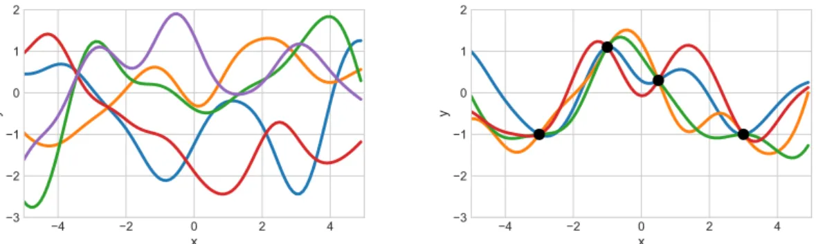
f and c leads to a distribution over linear functions. In Fig. 1.2, left, we show several functions drawn from a GP prior using a squared exponential kernel with variance and length scale parameters set to one.
4 2 0 2 4 x 3 2 1 0 1 2 y 4 2 0 2 4 x 3 2 1 0 1 2 y
Figure 1.2: Left: Functions drawn from a Gaussian process prior using a squared exponential kernel. Right: Functions drawn from the posterior of a GP regression model with no observation noise, after conditioning on four observations (black dots).
Latent Gaussian process models. In this thesis, we are interested in probabilistic models that consist of a latent function f that is defined on the data points X = (x1, . . . ,xn)> ∈ Rn×d. We assume a prior GP distribution on the latent function
likelihood p(y|f). The generative model is f ∼GP(0, k) y∼p(y|f, X) = n Y i=1 p(yi|f(xi)). (1.1)
In this thesis, we refer to this class of models as latent Gaussian process models. A wide range of models can be obtained by choosing different likelihood functions. For instance using a Gaussian likelihood
p(yi|f(xi)) =N(yi|f(xi), σ2), (1.2) where yi ∈ R and σ2 is an additional parameter, leads to the standard (Gaussian likelihood) GP regression model. A binary classification model can be obtained by using a Bernoulli likelihood
p(yi|f(xi)) =B(yi|σ(yif(xi))),
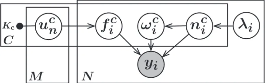
where yi ∈ {−1,1} and σ(.) is an activation function mapping the GP outputs to probabilities in the interval [0,1]. More complicated likelihoods can be obtained by considering models with additional latent variables z= (z1, . . . , zk) (e.g. hierarchical models). For instance, in Chapter 7 we propose a language model that has a hierar-chical structure based on a set of multiple latent GPs and additional latent variables, which model certain aspects of a text document (see Fig. 7.1).
For the sake of simplicity, in the following of the introduction, we only consider latent GP models of the form given in Eq. 1.1 and omit potential additional latent variables and assume a single latent GP f. Note that the ideas developed in the first two chapters also apply to models with multiple latent GPs and models with additional latent variables1.
In the following, we use the shorthand fi = f(xi) and omit that we are always conditioning on the data points X.
Inference in latent GP models. The main goal is to compute the posterior distribution of the latent GP, which, in principle, is given by Bayes’ rule
p(f|y) = p(y|f)p(f)
p(y) . (1.3)
1In particular, models with additional latent variables can still be viewed from the perspective of
having a single (complicated) likelihood in the form of Eq. 1.1 by considering the marginal likelihood p(y|f, X) =Rp(y|z, f, X)p(z|f, X)dz.
We can make predictions about unseen dataX∗ = (x∗1, . . . ,x∗k)>by first computing the distribution of the latent function values corresponding to the test cases
p(f∗|y, X∗) =
Z
p(f∗|f, X∗)p(f|y)df
and then using this distribution overf∗ to compute the predictive distribution
p(y∗|y, X∗) =
Z
p(y∗|f∗)p(f∗|y, X∗)df∗.
In the case of Gaussian GP regression, i.e. using the likelihood given in (1.2), the posterior and predictive distribution can be computed in closed form (Rasmussen and Williams, 2006). In this case, the likelihood is conjugate to the GP prior, that means that the posterior distribution is in the same family as the prior distribution. Hence, in the context of GP regression, the posterior of the function valuesf is again Gaussian distributed. Moreover, the predictive distribution is given by
p(y∗|y, X∗) = N(µ∗,Σ∗) (1.4) with µ∗ =K(X∗, X) K(X, X) +σ2I −1 y Σ∗ =K(X∗, X∗)−K(X∗, X) K(X, X) +σ2nI −1 K(X, X∗),
whereK(X, X0) denotes thekernel matrix resulting from evaluating the kernel func-tion between points X = (x1, . . . ,xN)> and X0 = (x01, . . . ,x0N0)>, which is given by
K(X, X0)ij =k(xi,x0j). In Fig. 1.2, right, we show functions drawn from the poste-rior predictive distribution (1.4) upon observing four data points in a GP regression model using a squared exponential kernel.
For other non-conjugate likelihoods, computing the posterior (1.3) is often in-tractable and requires approximate inference. Many different approaches to approxi-mate inference in GP models have been proposed including sampling based methods, e.g. elliptic slice sampling (Murray, Adams, and MacKay, 2010) and sampling us-ing control variates (Lawrence, Rattray, and Titsias, 2009), as well as variational methods, e.g. based on expectation propagation (Hern´andez-Lobato and Hern´ andez-Lobato, 2016) or variational inference (Hensman, Fusi, and Lawrence, 2013; Salim-beni, Eleftheriadis, and Hensman, 2018).
Another issue is that, even in the simple GP regression model, inference is slow and does not scale to big datasets. Due to the inversion of the kernel matrix, naive
inference in latent GP models typically has computational complexity O(n3), where n is the number of data points.
In this thesis, we focus on variational inference and discuss how these problems can be circumvented.
Variational inference. We employvariational inference to deal with the intractable posterior (1.3). Variational inference maps the infeasible inference problem to a fea-sible optimization problem (see e.g. Blei, Kucukelbir, and McAuliffe, 2017). The idea is to choose a family of tractable variational distributions qθ(f), where θ denote the variational parameters of the distribution family, and then select the best approxi-mation of the true posterior p(f|y) by minimizing the Kullback-Leibler divergence between the variational distribution and the posterior
KL(qθ(f)||p(f|y)) =Eqθ(f)[logqθ(f)−logp(f|y)]
with respect to the variational parametersθ. This is equivalent to maximizing a lower bound on the log marginal likelihood, known as evidence lower bound (ELBO)
L(θ) =Eqθ(f)[logp(y,f)−logqθ(f)]≤logp(y).
Sparse variational approximation. Sparse Gaussian processes address the issue of the cubic computational complexity of inference in GP models. Different ap-proaches to sparse approximations of GPs have been discussed in literature including the early work by Csat´o and Opper, 2002 and Csat´o, 2002, and Seeger, Williams, and Lawrence, 2003. Based on that work, we employ a variational approach and follow the line of research by Snelson and Ghahramani, 2005; Titsias, 2009; Hensman, Fusi, and Lawrence, 2013. We replace the latent GPf by a sparse approximation building on a set of inducing points. This reduces the complexity to O(m3), where m is the number of inducing points.
The sparse GP approximation is obtained as follows. We start with the latent GP model (1.1) and introduce an inducing-point augmentation to the latent GP f. The new random variable consists ofmadditional input-output pairs (z1, u1), . . . ,(zm, um), termed asinducing inputs and inducing variables. The function values of the GP f and the inducing variables u= (u1, . . . , um) are connected via
p(f|u) =N f|KnmKmm−1 u,Ke
p(u) =N (u|0, Kmm),
whereKmm is the kernel matrix resulting from evaluating the kernel function between all inducing inputs, Knm is the cross-kernel matrix between inducing inputs and training points, and Ke =Knn−KnmKmm−1 Kmn. Including the inducing points in our
model gives the augmented joint distribution
p(y,f,u) =p(y|f)p(f|u)p(u).
Note that the original model (1.1) can be recovered by marginalizing u.
We aim to approximate the posterior of the sparse GP p(u|y) and apply the methodology of variational inference to the augmented joint distribution p(y,u,f). We assume the variational distribution family q(u,f) = q(u)p(f|u), where q(u) =
N(u|m, S) is a variational Gaussian distribution with variational mean parameter mand variational covariance parameter S. Note that the factor p(f|u) is fixed and given by Eq. 1.5.
The final variational lower bound on the evidence (ELBO) is given by
logp(y)≥Ep(f|u)q(u)[logp(y|f)]−KL (q(u)||p(u)). (1.6)
The inducing point locations Z are additional hyperparameters and are either fixed or optimized via maximizing the fitted variational lower bound as a function of the inducing point locations (see Section 2.2).
Chapter 2
Augmented Variational Inference
for Gaussian Process Models
In this chapter, we propose an unified framework for efficient inference in latent GP models. Inference in latent GP models that go beyond simple regression is chal-lenging due to the non-conjugate likelihood. Previous scalable inference methods (e.g. Hensman and Matthews, 2015; Dezfouli and Bonilla, 2015; Hern´andez-Lobato and Hern´andez-Lobato, 2016; Salimbeni, Eleftheriadis, and Hensman, 2018) typically build on approximating the likelihood by sampling or numerical quadrature, thus, preventing efficient optimization.
We develop a different approach that aims on translating the intractable non-conjugate model into an easier conditionally non-conjugate model by adding auxiliary random variables to the model. An auxiliary variable is an additional latent variable that is added to a model such that the original model is recovered when this vari-able is marginalized out. We aim to find an augmentation that renders the model conditionally conjugate. Inference in the augmented conditionally conjugate model is much easier than in the original model. We develop an efficient variational inference method based on block coordinate updates, which can be computed in closed form. The updates correspond to natural gradient updates, which are more efficient than ordinary Euclidean gradient updates, which are used in previous approaches.
In the following of this chapter, we introduce the main ideas behind our new
augmented variational inference approach. This chapter is meant to provide a high-level motivation of our approach and focuses on the general concepts. In part II of the thesis, we show that this framework is actually useful in practice. We study five different latent GP models and develop scalable inference methods based on the principles laid out in this chapter.
y X f z X y f z ω
Conditionally conjugate augmentation
Non-conjugate GP model Variational inference updates
in closed-form
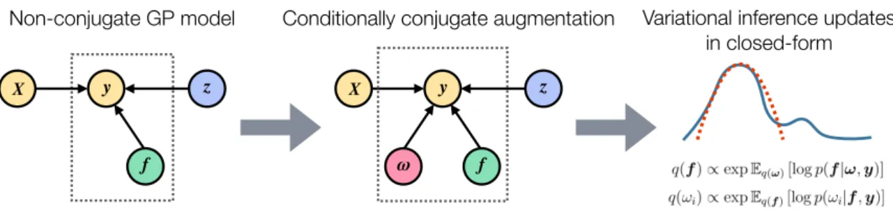
Figure 2.1: How can we perform scalable inference in latent Gaussian process models? We propose an augmented variational inference approach, which leads to efficient variational inference updates given in closed form. We start with the non-conjugate latent GP model (left), where the latent GP is denoted by f, (optional) additional random variables are denoted by z and the data is (X, y). In the first step, we add auxiliary random variables ω to the model that render the model conditionally conjugate (middle). In the conditionally conjugate model, all complete conditional distributions (the posterior distribution of one random variable given all the others) are tractable. In the last step (right), we obtain an approximation of the posterior. We leverage conditional conjugacy to derive efficient variational inference updates, which are given in closed form.
2.1
A conditionally conjugate formulation via
aux-iliary variable augmentation
The main idea of the augmented variational inference approach is to add auxiliary random variables to the latent GP model such that inference becomes easier. In particular, we aim to find an augmented representation of the model that renders the model conditionally conjugate. Let ω = (ω1, . . . , ωn) be a set of auxiliary random variables, which augment the original model (1.1) leading to a joint distribution of the form
p(y,f,ω) = Y i
p(yi|fi, ωi)p(ωi)p(f). (2.1)
The original model can be restored by marginalizingω, i.e. p(y,f) =R p(y,f,ω)dω. In our work, the goal is to find an augmentation ω such that the augmented likelihood p(y|f,ω) becomes conjugate to the prior distributions p(f) and p(ω), i.e. the complete conditional distributionsp(f|ω,y) andp(ω|f,y) are in the same family as their associated priors. Furthermore, we seek for an augmentation the allows us to compute expectations of the log complete conditional distributions, given in Eq. 2.3, in closed form. Later we will see that these requirements are sufficient for obtaining efficient variational inference updates (see Eq. 2.3).
As a direct consequence from the above requirements, we seek for augmentations that render the likelihood to be a squared exponential function in fi, i.e.
p(yi|fi, ωi)∝exp a(yi, ωi) +b(yi, ωi)fi+c(yi, ωi)fi2, (2.2) whereaandb are arbitrary factors that only depend on the label yi and the auxiliary variable ωi. An augmented likelihood of this form leads to a Gaussian complete conditional p(f|ω,y). Additional to the conditional conjugacy in f, we seek for an augmentation that also leads to a tractable complete conditional distribution in the augmented variables p(ω|f,y).
To summarize, our method is based on finding a suitable augmentation of the original model. In this section, we have established the requirements that define a
suitable augmentation. The goal is to find an augmentation ω, which
• renders the model conditionally conjugate and
• allows us to compute expectations of the complete conditionals (given in Eq. 2.3) in closed-from.
These goals serve as a guide in the process of finding suitable augmentations. In the next chapters, we will see that such augmentations can be indeed found for a variety of different models and lead to a substantial decrease in computation time when performing variational inference.
Note that a suitable augmentation can involve more than one set of auxiliary variables. For instance, in Chapter 4 we develop a hierarchical augmentation of a multi-class GP classification model, which involves three different sets of auxiliary variables. For the sake of simplicity, in this chapter, we focus on the case of having one set of auxiliary variables ω = (ω1, . . . , ωn) that factorizes the likelihood in the form of Eq. 2.1.
2.2
Variational inference in the augmented model
For now, let us assume we have found an augmentationωthat fulfills the requirements defined in Section 2.1. We show that in this case, the posterior can be efficiently approximated using variational inference.
We assume a variational distribution where the latent GPf and the augmentation variables are decoupled, i.e. q(f,ω) = q(f)q(ω). Following standard results (Blei, Kucukelbir, and McAuliffe, 2017), the optimal variational distribution ofωfactorizes,
i.e. q(ω) =Q
iq(ωi) and the variational distributions can be iteratively optimized by the block-coordinate ascent updates given by
q(f)∝expEq(ω)[logp(f|ω,y)]
q(ωi)∝expEq(f)[logp(ωi|f,y)].
(2.3) The assumptions from the previous section imply that these updates are computed in closed form. Furthermore, from the structure of the augmented likelihood (2.2), it fol-lows that the variational distributionq(f) is in the same family as the corresponding complete conditional and, thus, q(f) is a variational Gaussian distribution.
In order to scale to big datasets we employ stochastic variational inference (Hoff-man et al., 2013) and replace the original latent GPf by a sparse approximationuas introduced in Section 1.2. Hoffman et al., 2013 have shown in the setting, where the complete conditionals are in the exponential family, that the coordinate updates (2.3) can be directly interpreted as natural gradient updates with a learning rate of one. In stochastic variational inference, the variational objective is optimized via stochastic optimization based on stochastic natural gradients. In each iteration, we use mini-batches of the data and obtain a noisy version of the natural gradient. In this setting, learning rates slightly less than one have to be chosen.
Optimization of hyperparameters. The hyperparameters of our model include kernel hyperparameters and inducing point locations. The hyperparameters can be either fixed before training or optimized via a variational expectation maximization (EM) approach.
We select the optimal kernel hyperparameters by maximizing the marginal like-lihood p(y|h), where h denotes the set of hyperparameters (this approach is called empirical Bayes (Maritz and Lwin, 1989)). We follow an approximate approach and optimize the fitted variational lower bound L(h) as a function ofh by alternating be-tween optimization steps w.r.t. the variational parameters and the hyperparameters (see e.g. Mandt, Hoffman, and Blei, 2016).
2.3
On the quality of the augmented
approxima-tion
The main advantage of theaugmented variational inferenceapproach is, that it leads to variational updates that are computed in closed form and can be interpreted as efficient block coordinate updates. Hence, our inference method is often faster and
more stable than competing methods that apply variational inference to the original (non-augmented) latent GP model.
The price we have to pay for faster inference is an additional approximation error compared to the variational inference solution of the original model. In this section, we discuss the additional augmentation gap of the ELBO introduced by the auxiliary variablesω. For the sake of simplicity, we consider here the non-sparse case, i.e. the inducing points equal the training points (f =u). However, it is straightforward to extend the results also to the sparse case.
In a direct application of variational inference to the latent GP model (Eq. 1.1), one tries to approximate the posterior directly by a variational Gaussian q∗(f) =
N(f|µ∗,Σ∗) without using an auxiliary variable augmentation. This leads to the
optimization problem arg min
q(f)
KL(q(f)||p(f|y)) = arg max q(f) E
q(f)[logp(y,f)−logq(f)].
Optimizing the original ELBO Lorig(q) (right-hand side of the equation above) is in
general not tractable. For some models, e.g. GP classification models (Hensman and Matthews, 2015), the ELBO can be approximated by sampling or numerical quadrature. For the sake of the analysis, we now assume that we have an algorithm that allows us to optimize the original ELBO and we denote the optimizer with qorig∗ (f).
In our approach, we apply variational inference to the augmented model and optimize theaugmented ELBO
Laugmented(q) = Eq(f)q(ω)[logp(y,f,ω)−logq(f)−logq(ω)].
We look for the best distribution q∗(f,ω) = q∗(f)q∗(ω) that factorizes in the aug-mented auxiliary variablesω and the original functionf. This approach also yields a Gaussian approximationq∗(f) as a factor in the optimal density. Of courseq∗(f) will be different from the “optimal” approximation qorig∗ (f) that maximizes the original ELBO.
It would be interesting to see how the maximized ELBOs of the two variational approaches, which both give a lower bound on the likelihood of the data, differ. Un-fortunately, such a computation would require the knowledge of the optimalqorig∗ (f). However, we can obtain some estimate of this difference by directly comparing both
bounds using the sameGaussian density q(f). In this case, we obtain
Lorig(q(f))− Laugmented(q(f)q(ω))
=Eq(f)[logp(y,f)−logq(f)]−Eq(f)q(ω)[logp(y,f,ω)−log(q(f)q(ω))]
=Eq(f)q(ω)[logp(y|f)−logp(y|f,ω)−logp(ω) + logq(ω)]
=Eq(f)q(ω)[−logp(ω|f,y) + logq(ω)]
=Eq(f)[KL (q(ω)||p(ω|f,y))].
The augmentation gap is small if, on average, the variational approximation q(ω) is close to the posteriorp(ω|f,y).
We could, however, argue that asymptotically, in the limit of a large number of data, the predictions given by both densities may not differ a lot, as the posterior uncertainty for both densities should become small. Neglecting this uncertainty in the expectation of the log-likelihood in the Gaussian variational approximation shows that the approximation of the posterior mean in q∗(f) becomes equal to the MAP estimator (Opper and Archambeau, 2009). If we neglect the posterior uncertainty (and the extra error caused by sparsity) in our approximation, we simply arrive at anexactEM algorithm for computing the same MAP estimator of the model. This is because in the E-step, we can compute the expectation over the augmentation vari-ables ω exactly. We might, however, get some difference in the covariance structure of the two Gaussian densitiesq∗(f) and q(f), which is not expected to cause a major deterioration of the predictions.
For the latent GP models discussed in the next chapters, we confirm empirically that the additional approximation error is small in practice and the predictive per-formance of our approach is competitive.
2.4
Gibbs sampling
Since our augmented model is conditionally conjugate we can directly derive a Gibbs sampling scheme. In order to sample from the exact posterior, we alternate between drawing a sample from each complete conditional distribution
ft∼p(f|ωt−1,y)
and
whereω0is appropriately initialized. The augmented variables are naturally
marginal-ized out and asymptotically, the latent GP samples will be from the true posterior. In this thesis, we focus on the methodology of variational inference since it can be scaled to big datasets more easily. However, the Gibbs sampling scheme is a useful tool to empirically assess the quality of our approximate posterior on small datasets.
Part II
Scalable Inference in Latent
Gaussian Process Models
Chapter 3
Gaussian Process Classification
We begin our study of latent GP models with a GP classification model. We propose a scalable stochastic variational approach building on P´olya-Gamma data augmenta-tion and inducing points. Unlike previous approaches, we obtain closed-form updates based on natural gradients, which lead to efficient optimization. We evaluate the algo-rithm on real-world datasets containing up to 11 million data points and demonstrate that it is up to two orders of magnitude faster than the state of the art while being competitive in terms of prediction performance. The code is available via Github1.
This chapter is based on:
F. Wenzel∗, T. Galy-Fajou∗, C. Donner, M. Kloft, and M. Opper (2019). “Efficient
Gaussian Process Classification Using P´olya-gamma Data Augmentation”. In: AAAI
Conference on Artificial Intelligence.
We consider a binary GP Classification model, which is defined as follows. Let X = (x1, . . . ,xn)> ∈ Rn×d be the d-dimensional training points with labels y =
(y1, . . . , yn)∈ {−1,1}n. The likelihood of the labels is p(y|f) =
n
Y
i=1
σ(yif(xi)), (3.1)
wheref ∼GP(0, k) is a latent GP function andσ(z) is an activation function, which maps the latent function values to the interval [0,1]. In our work, we consider the logistic function σ(z) = (1 + exp(−z))−1.
Currently, GP classification has limited applicability to big data. Naive inference typically scales cubically in the number of data points, and exact computation of the posterior and marginal likelihood is intractable.
1https://github.com/theogf/AugmentedGaussianProcesses.jl ∗Equal contributions.
Nevertheless, the combination of so-called sparse Gaussian process techniques (cf. Section 1.2) with approximate inference methods, such as expectation propagation (EP) or the variational approach, have enabled GP classification for datasets contain-ing millions of data points (Hern´andez-Lobato and Hern´andez-Lobato, 2016; Salim-beni, Eleftheriadis, and Hensman, 2018).
While these results are already impressive, we will show that our augmented vari-ational inferenceapproach leads to a speed-up of up to two orders of magnitude. We show that the logistic GP classification model can be augmented by P´olya-Gamma random variables (Polson, Scott, and Windle, 2013) leading to a conditionally conju-gate model.
As outlined in Section 2.1, the augmentation approach gives directly rise to coor-dinate ascent updates and the optimization procedure can be interpreted as a natural-gradient approach to variational inference. Unlike previous approaches, the natural gradient updates can be computed in closed form leading to a fast and stable algo-rithm, which is simple to implement.
3.1
Background and related work
Gaussian process classification. Hensman and Matthews (2015) consider Gaus-sian process classification with a probit inverse link function and suggest a variational Gaussian model that builds on inducing points. By employing automatic differentia-tion, Salimbeni, Eleftheriadis, and Hensman (2018) generalize this approach to apply natural gradients in non-conjugate GP models. Khan and Nielsen (2018) consider natural gradient updates in the setting of variational inference with exponential fam-ilies. Unlike our approach, these methods do not benefit from closed-form updates and have to resort to numerical approximations. Moreover, our approach has the advantage that a higher learning rate close to one can be chosen since our updates can be interpreted as block-coordinate ascent updates.
Izmailov, Novikov, and Kropotov, 2018 use tensor train decomposition to train GP models with billions of inducing points. The updates are not computed in closed form and they do not use natural gradients.
Dezfouli and Bonilla (2015) propose a general automated variational inference approach for sparse GP models with non-conjugate likelihoods. Since they follow a black box approach and do not exploit model specific properties, they do not employ efficient optimization techniques.
Hern´andez-Lobato and Hern´andez-Lobato (2016) follow an expectation propaga-tion approach based on inducing points and have a similar computapropaga-tional cost as Hensman and Matthews (2015).
P´olya-Gamma data augmentation. Polson, Scott, and Windle (2013) intro-duced the idea of data augmentation in logistic models using the class of P´ olya-Gamma distributions. This allows for exact inference via Gibbs sampling or approx-imate variational inference schemes (Scott and Sun, 2013).
Linderman, Johnson, and Adams (2015) extend this idea to multinomial models and discuss the application for Gaussian processes with multinomial observations but their approach does not scale to big datasets and they do not consider the concept of inducing points.
3.2
The augmentation
Due to the analytically inconvenient form of the likelihood function, inference for lo-gistic GP classification is a challenging problem. We remedy this issue by considering an augmented representation of the original model. The augmented model is ad-vantageous since it leads to efficient closed-form updates in our variational inference scheme.
Polson, Scott, and Windle (2013) introduced the class of P´olya-Gamma random variables and proposed a data augmentation strategy for inference via Gibbs sampling in models with binomial likelihoods. The augmented model has the appealing prop-erty that the likelihood of the latent function valuesf is proportional to a Gaussian density when conditioned on the augmented P´olya-Gamma variables. Furthermore, the auxiliary P´olya-Gamma variables conditioned on the GP valuesf are again P´ olya-Gamma distributed. The P´olya-Gamma augmentation satisfies our requirements from Section 2.1 and hence can be utilized to derive an efficient approximate inference al-gorithm.
The P´olya-Gamma distribution is defined as follows. The random variable ω ∼
PG(b,0), b >0 is defined by the moment generating function
EPG(ω|b,0)[exp(−ωt)] =
1
coshb(pt/2). (3.2) It can be shown that this is the Laplace transform of an infinite convolution of gamma distributions. The definition is related to our problem by the fact that the logistic likelihood can be written in a form that involves thecosh(.) function, namelyσ(zi) =
exp(12zi)(2 cosh(z2i))−1. In the following we derive a representation of the logistic likelihood in terms of P´olya-Gamma variables.
First, we define the general PG(b, c) class that is derived by an exponential tilting of the PG(b,0) density, and it is given by
PG(ω|b, c)∝exp(−c
2
2ω)PG(ω|b,0).
From the moment generating function (3.2), the first moment can be directly com-puted EP G(ω|b,c)[ω] = b 2ctanh c 2 .
For the subsequently presented variational algorithm, these properties suffice and the full representation of the P´olya-Gamma density PG(ω|b, c) is not required.
We now adapt the data augmentation strategy based on P´olya-Gamma variables for the GP classification model. To do this, we write the non-conjugate logistic likelihood function (3.1) in terms of P´olya-Gamma variables
σ(zi) = (1 + exp(−zi)) −1 = exp( 1 2zi) 2 cosh(zi 2) = 1 2 Z exp zi 2 − z2 i 2ωi p(ωi)dωi, (3.3) where p(ωi) = PG(ωi|1,0) and by making use of (3.2). For more details see Polson, Scott, and Windle (2013). Using this identity and substituting zi = yif(xi) we augment the joint densityp(y,f) with P´olya-Gamma variables and obtain
p(y,f,ω)∝exp 1 2y > f − 1 2f > Ωf p(f)p(ω), (3.4) where Ω = diag(ω) is the diagonal matrix of the P´olya-Gamma variables {ωi}.
Interestingly, employing a structured mean field variational inference approach (cf. Section 3.3) to the plain P´olya-Gamma augmented model (3.4) leads to the same bound for GP classification derived by Gibbs and MacKay (2000). This is an inter-esting new perspective on this bound since they do not employ a data augmentation approach. We provide a proof in Appendix A.3. Our approach goes beyond Gibbs and MacKay (2000) by providing a fully Bayesian perspective, including a sparse GP prior in the model and proposing a scalable inference algorithm based on natural gradients (Section 3.3).
3.3
Inference
To scale our model to big datasets, we approximate the latent GP f by a sparse GP
building on inducing points. As outlined in Section 1.2, we introduce M inducing points u and connect the GP values with the inducing points via the joint prior distributionp(f,u) = p(f|u)p(u) given in Eq. 1.5.
We follow a structured mean field approach (Wainwright and Jordan, 2008) and assume independence between the inducing variablesu and P´olya-Gamma variables ω, yielding a variational distribution of the form q(u,ω) = q(u)q(ω). Setting the functional derivative of L w.r.t. q(u) and q(ω) to zero, respectively, results in the following consistency condition for the maximum,
q(u,ω) =q(u)Y i
q(ωi), (3.5)
withq(ωi) = PG(ωi|1, ci) and q(u) =N(u|µ,Σ). Remarkably, we do not have to use the full P´olya-Gamma class PG(ωi|bi, ci), but instead, consider the restricted class bi = 1 since it already contains the optimal distribution. This can be easily seen by starting with a free-form mean field variational inference approach and deriving the optimal conditionbi = 1.
Using (3.5) as variational family, which is parameterized by the variational pa-rameters {µ,Σ,c} leads to a closed-form expression of the variational bound
L(c,µ,Σ)
=Ep(f|u)q(u)q(ω)[logp(y|ω,f)]−KL (q(u,ω)||p(u,ω))
c = 1 2 log|Σ| −log|Kmm|)−tr(Kmm−1 Σ)−µ > Kmm−1 µ +X i n yiκiµ−θi e Kii−κiΣκ>i −µ > κ>i κiµ +c2iθi −2 log cosh ci 2 o , (3.6) whereθi = 21citanh c2i
andκi =KimKmm−1 . Remarkably, all intractable terms involv-ing expectations of log PG(ωi|1,0) cancel out. Details are provided in Appendix A.1.
Stochastic variational inference. Our algorithm alternates between updates of the local variational parametersc and global parameters µand Σ. In each iteration, we update the parameters based on a mini-batch of the data S ⊂ {1, . . . , n} of size s=|S|.
We update the local parameters cS in the mini-batch S by employing coordinate
ascent. To this end, we fix the global parameters and analytically compute the unique maximum of (3.6) w.r.t. the local parameters, leading to the updates
ci = q e Kii+κiΣκ>i +µ>κ > i κiµ (3.7) fori∈ S.
We update the global parameters by employing stochastic optimization of the variational bound (3.6). The optimization is based on stochastic estimates of the natural gradients of the global parameters. We use the natural parameterization of the variational Gaussian distribution, i.e., the parameters η1 := Σ−1µ and η2 =−12Σ−1.
Using the natural parameters results in simpler and more effective updates. The natural gradients based on the mini-batch S are given by
e ∇η1LS = n 2sκ > SyS−η1 e ∇η2LS =− 1 2 Kmm−1 + n sκ > SΘSκS −η2, (3.8)
where Θ = diag(θ) and θi = 21c
itanh
ci 2
. The factor ns is due to the rescaling of the mini-batches. The global parameters are updated according to a stochastic natural gradient ascent scheme. We employ the adaptive learning rate method described by Ranganath et al. (2013).
The natural gradient updates always lead to a positive definite covariance ma-trix2 and in contrast to Hensman and Matthews (2015) our implementation does not
require any assurance for positive-definiteness of the variational covariance matrix Σ. Details for the derivation of the updates can be found in Appendix A.2. The complexity of each iteration in the inference scheme isO(m3), due to the inversion of the matrix η2.
Predictions. The approximate posterior of the GP values and inducing variables is given by q(f,u) = p(f|u)q(u), where q(u) = N(u|µ,Σ) denotes the optimal variational distribution. To predict the latent function valuesf∗ at a test pointx∗ we
substitute our approximate posterior into the standard predictive distribution p(f∗|y) = Z p(f∗|f,u)p(f,u|y)dfdu ≈ Z p(f∗|f,u)p(f|u)q(u)dfdu = Z p(f∗|u)q(u)du=N f∗|µ∗, σ∗2 , (3.9)
where the prediction mean and the variance is µ∗ =K∗mKmm−1 µ
σ2∗ =K∗∗+K∗mKmm−1 (ΣK
−1
mm−I)Km∗.
The matrix K∗m denotes the kernel matrix between the test point and the inducing points and K∗∗ the kernel value of the test point. The distribution of the test labels
is easily computed by applying the logistic likelihood to (3.9), p(y∗ = 1|y) =
Z
σ(f∗)p(f∗|y)df∗. (3.10)
This integral is analytically intractable but can be computed numerically by quadra-ture methods. This is adequate and fast since the integral is only one-dimensional.
Computing the mean and the variance of the predictive distribution has complex-ity O(m) and O(m2), respectively.
Optimization of the hyperparameters. We select the optimal kernel hyperpa-rametershby maximizing the marginal likelihoodp(y|h) via a variational expectation maximization approach. The details are described in Section 1.2.
3.4
Experiments
We compare our proposed method, efficient Gaussian process classification (x-gpc), with the state-of-the-art methods svgpc (Salimbeni, Eleftheriadis, and Hensman, 2018), provided in the package GPflow3(Matthews et al., 2017), which builds on
Ten-sorFlow and the EP approach epgpc by Hern´andez-Lobato and Hern´andez-Lobato (2016), implemented in R. All methods are applied to real-world datasets containing up to 11 million data points.
In all experiments, a squared exponential covariance function with a common length scale parameter for each dimension, an amplitude parameter and an additive noise parameter is used. The kernel hyperparameters are initialized to the same values and optimized using Adam (Kingma and Ba, 2015), while inducing points location are initialized via k-means++ (Arthur and Vassilvitskii, 2007) and kept fixed during training. The SVI based methods,x-gpc and svgpc, use an adaptive learning rate. All algorithms are run on a single CPU. We experiment on 12 datasets from the OpenML website and the UCI repository ranging from 768 to 11 million data points.
Figure 3.1: Posterior mean (µ), variance (σ) and predictive marginals (p) on the Diabetes dataset. Each plot shows the MCMC ground truth on the x-axis and the estimated value of our model on the y-axis. Our approximation is very close to the ground truth.
In the first experiment (Section 3.4.1), we examine the quality of the approximation provided byx-gpc. In the next experiment, we evaluate the prediction performance and run time of x-gpc, andsvgpcandepgpcon several real-world datasets. Finally, in Section 3.4.3, we examine the sensitivity of all methods to the number of inducing points.
3.4.1
Quality of the approximation
We empirically examine the quality of the variational approximation provided by our method. In Fig. 3.1, we compare the approximations to the true posterior obtained by employing an asymptotically exact Gibbs sampler as described in Section 2.4 and also discussed by Polson and Scott, 2011; Linderman, Johnson, and Adams, 2015. We compare the posterior mean and variance as well as the prediction probabilities with the ground truth. Since the Gibbs sampler does not scale to large datasets we experiment on the small Diabetes dataset (n = 768). In Fig. 3.1 we plot the approximated values vs. the ground truth. We find that our approximation is very close to the true posterior.
3.4.2
Numerical comparison
We evaluate the prediction performance and run time of our method x-gpc and the competing methods svgpc and epgpc. We experiment on a variety of different datasets and report the resulting prediction error, negative test log-likelihood and run time for each method in Table 3.1.
The experiments are conducted as follows. For each dataset, we perform a 10-fold cross-validation and for datasets with more than one million points, we limit the
Dataset X-GPC SVGPC EPGPC aXa Error 0.17±0.07 0.17±0.07 0.17±0.07
n= 36,974 NLL 0.29±0.13 0.36±0.13 0.34±0.13 d= 123 Time 47±2.2 451±7.8 214±4.8 Bank Market. Error 0.14±0.12 0.12±0.12 0.12±0.13
n= 45,211 NLL 0.27±0.22 0.31±0.26 0.33±0.20 d= 43 Time 9±1.5 205±6.6 46±3.5 Click Pred. Error 0.17±0.00 0.17±0.00 0.17±0.01
n= 399,482 NLL 0.39±0.07 0.46±0.00 0.46±0.01 d= 12 Time 4.5±1.3 102±3.0 8.1±0.45 Cod RNA Error 0.04±0.00 0.04±0.00 0.04±0.00
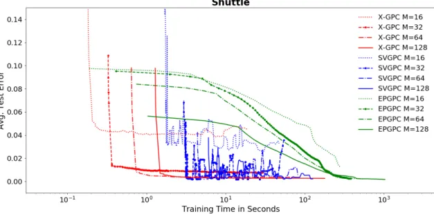
n= 343,564 NLL 0.11±0.03 0.13±0.00 0.12±0.00 d= 8 Time 3.7±0.13 115±4.3 869±5.2 Diabetes Error 0.23±0.07 0.23±0.06 0.24±0.06 n= 768 NLL 0.47±0.11 0.47±0.10 0.48±0.09 d= 8 Time 8.8±0.12 150±5.1 8±0.45 Electricity Error 0.24±0.06 0.26±0.06 0.26±0.06 n= 45,312 NLL 0.31±0.17 0.53±0.08 0.53±0.06 d= 8 Time 8.2±0.48 356±6.9 13.5±1.50 German Error 0.25±0.12 0.25±0.11 0.26±0.13 n= 1,000 NLL 0.44±0.17 0.51±0.15 0.53±0.11 d= 20 Time 17±0.42 374±7.3 5.2±0.03 Higgs Error 0.33±0.01 0.45±0.01 0.38±0.01 n= 11,000,000 NLL 0.55±0.13 0.69±0.00 0.66±0.00 d= 28 Time 23±0.88 294±54 8732±867 IJCNN Error 0.03±0.01 0.06±0.01 0.02±0.01 n= 141,691 NLL 0.10±0.03 0.15±0.07 0.09±0.04 d= 22 Time 17±0.44 1033±45 756±8.6 Mnist Error 0.14±0.01 0.44±0.13 0.12±0.01 n= 70,000 NLL 0.24±0.10 0.66±0.11 0.27±0.01 d= 780 Time 200±5.5 991±23 806±5.2 Shuttle Error 0.01±0.01 0.01±0.00 0.01±0.01 n= 58,000 NLL 0.07±0.01 0.07±0.00 0.07±0.01 d= 9 Time 0.01±0.00 7.5±0.7 100±0.63 SUSY Error 0.21±0.00 0.22±0.00 0.22±0.00 n= 5,000,000 NLL 0.31±0.10 0.49±0.01 0.50±0.00 d= 18 Time 14±0.29 10,000 10,000 wXa Error 0.03±0.01 0.04±0.01 0.03±0.01 n= 34,780 NLL 0.27±0.07 0.25±0.07 0.19±0.06 d= 300 Time 66±16 612±11 1.4±0.10
Table 3.1: Average test prediction error, negative test log-likelihood (NLL) and time in seconds along with one standard deviation. Best values are highlighted.
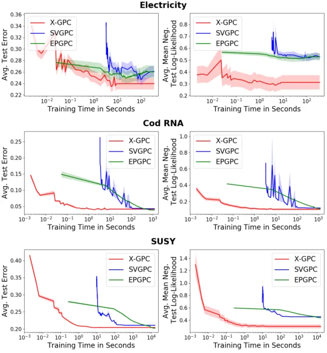
Figure 3.2: Average negative test log-likelihood and average test prediction error as a function of training time (seconds in a log10 scale) on the datasets Electricity (45,312 points), Cod RNA (343,564 points) and SUSY (5 million points). x-gpc (proposed) reaches values close to the optimum after only a few iterations, whereas svgpc and epgpc are one to two orders of magnitude slower.