Copyright belongs to the author. Small sections of the text, not exceeding three paragraphs, can be used provided proper acknowledgement is given.
The Rimini Centre for Economic Analysis (RCEA) was established in March 2007. RCEA is a private, nonprofit organization dedicated to independent research in Applied and Theoretical Economics and related
fields. RCEA organizes seminars and workshops, sponsors a general interest journal The Review of
Economic Analysis, and organizes a biennial conference: The Rimini Conference in Economics and Finance
(RCEF). The RCEA has a Canadian branch: The Rimini Centre for Economic Analysis in Canada
(RCEA-Canada). Scientific work contributed by the RCEA Scholars is published in the RCEA Working Papers and
Professional Report series.
The views expressed in this paper are those of the authors. No responsibility for them should be attributed to
the Rimini Centre for Economic Analysis.
The Rimini Centre for Economic Analysis
Legal address: Via Angherà, 22 – Head office: Via Patara, 3 - 47900 Rimini (RN) – Italy www.rcfea.org -
[email protected]
WP 10-51
Dimitris Korobilis
Université Catholique de Louvain
The Rimini Centre for Economic Analysis (RCEA)
VAR
F
ORECASTING
U
SING
B
AYESIAN
VAR forecasting using Bayesian variable selection
Dimitris KorobilisUniversité Catholique de Louvain
Abstract
This paper develops methods for automatic selection of variables in Bayesian vector autoregressions (VARs) using the Gibbs sampler. In particular, I provide computationally efficient algorithms for stochastic variable selection in generic linear and nonlinear models, as well as models of large dimensions. The performance of the proposed variable selection method is assessed in forecasting three major macroeconomic time series of the UK econ-omy. Data-based restrictions of VAR coefficients can help improve upon their unrestricted counterparts in forecasting, and in many cases they compare favorably to shrinkage esti-mators.
Keywords: Forecasting; variable selection; time-varying parameters; Bayesian vector au-toregression
JEL Classification: C11, C32, C52, C53, C66, E37
Center for Operations Research and Econometrics, Université Catholique de Louvain, and the Rimini Center for Economic Analysis. Address for correspondence: CORE, 34 Voie du Roman Payes, B-1348, Louvain-la-Neuve, Belgium. Tel: +32 (0)10 47.43.51.
1
Introduction
Since the pioneering work of Sims (1980), a large part of empirical macroeconomic model-ing is based on vector autoregressions (VARs). Despite their popularity, the flexibility of VAR models entails the danger of over-parameterization, which can lead to poor forecasts. This pitfall of VAR modelling was recognized early, and in response shrinkage methods have been proposed; see for example the so-called Minnesota prior (Doan, Litterman and Sims, 1984). Nowadays the applied econometricians’ toolbox includes numerous efficient modelling tools to prevent the proliferation of parameters and eliminate parameter and model uncertainty: vari-able selection priors (George, Sun and Ni, 2008), steady-state priors (Villani, 2009), Bayesian model averaging (Garratt, Koop, Mise and Vahey, 2009) and factor models (Stock and Watson, 2006), to name but a few.
This paper develops a stochastic search algorithm for variable selection in linear and non-linear vector autoregressions (VARs) using Markov Chain Monte Carlo (MCMC) methods. The term “stochastic search” simply means that if the model space is too large to assess in a de-terministic manner (that is, enumerate and estimate all possible models, and decide on the best one using some goodness-of-fit measure), the algorithm will visit only the most proba-ble models in a stochastic manner. In this paper, the general model form that I am studying is the reduced-form VAR model, which can be written using the following linear regression specification
yt=c+B1yt 1+B2yt 2+:::+Bpyt p+"t (1)
whereytis anm 1vector oft= 1; :::; T time series observations on the dependent variables
and the errors"tare assumed to beN(0; ), where is anm mcovariance matrix. The idea
behind Bayesian variable selection is to introduce indicators ij such that
Bij = 0 if ij = 0 (2)
Bij 6= 0 if ij = 1
where Bij is an element of the m k coefficient matrix B = c; B10; :::; Bp0 , for i = 1; ::; m,
j= 1; :::; kandk=p+ 1.
There are various benefits of using this approach over some of the shrinkage methods mentioned previously, such as the Minnesota prior or factor models. First, variable selection is automatic, meaning that along with estimates of the parameters we get associated probabilities of inclusion of each parameter in the “best” model. In that respect, the variables ij indicate which elements ofB should be included or excluded from the final optimal model. Selection of the optimal model is implemented among all possible2n,n=mk, VAR model combinations, without the need to estimate each and every one of these models. Second, this form of Bayesian variable selection is independent of the prior assumptions about the coefficients B. That is, if the researcher has defined any desirable prior for the parameters of the unrestricted model (1), adopting the variable selection restriction (2) needs no other modification than adding one extra block in the posterior sampler that draws from the conditional posterior of the ij’s. An
indirect implication of this approach is that, unlike other proposed stochastic search variable selection algorithms for VAR models (George et al. 2008; Korobilis, 2008), variable selection of this form may be adopted in VAR models which are nonlinear in the mean coefficientsB.
In fact, in this paper I show that variable selection is very easy to adopt in the non-linear and richly parameterized, time-varying parameters vector autoregression (TVP-VAR). These models are currently very popular for measuring monetary policy and have been used exten-sively in academic research (Canova and Gambetti, 2009; Cogley and Sargent, 2002; Cogley, Morozov and Sargent, 2005; Koop, Leon-Gonzalez and Strachan, 2009; and Primiceri, 2005). Common feature of these papers is that they all fix the number of autoregressive lags to 2 for parsimony. This simplification is so popular because marginal likelihoods are difficult to obtain, especially in the presence of stochastic volatility where one has to rely on computation-ally expensive particle filtering methods (Koop and Korobilis, 2009a). Even if we assume that marginal likelihoods are readily available, these would allow only pairwise comparisons and hence all2n TVP-VAR models need to be estimated. Therefore, automatic variable selection is
a convenient and fast way to overcome the computational and practical problems associated with (computationally) demanding nonlinear VAR models as well as simple linear models.
Apart from the TVP-VAR I examine closely the performance of Bayesian variable selection on several VAR formulations with various prior specifications. In particular I begin with the simple linear VAR model with ridge regression, Minnesota, and adaptive shrinkage priors. Fol-lowing this, variable selection for nonlinear models is introduced, where in addition to the TVP-VAR I consider a multivariate extension of the Koop and Potter (2007) structural breaks autoregressive model which allows to forecast breaks out-of-sample. Finally, given the recent interest in forecasting with large models (Ba´nbura, Giannone and Reichlin, 2010) as an alter-native to dimension reduction using principal components (Stock and Watson, 2006), a modi-fication of the stochastic restriction search useful for VARs of medium and large dimensions is established.
Although the methods described in this paper can be used for structural analysis (by pro-viding data-based restrictions on the coefficients which could enhance identifying monetary policy for instance), the aim is to show how more parsimonious models can be selected to have a positive impact on macroeconomic forecasting.
The next section describes the mechanics behind variable selection in VAR and TVP-VAR models. In Section 3, the performance of the variable selection algorithm is assessed using a small Monte Carlo exercise. The paper concludes by evaluating the out-of-sample forecasting performance of VAR models using variable selection, by computing pseudo-forecasts of 4 UK macroeconomic variables over the sample period 1971:Q1 - 2008:Q4.
2
Variable selection in vector autoregressions
To allow for different equations in the VAR to have different explanatory variables, rewrite equation (1) as a system of seemingly unrelated regressions (SUR)
yt=zt +"t (3)
where zt = Im xt = Im (1; yt 1; :::; yt p) is a matrix of dimensions m n, = vec(B0)
isn 1, and "t N(0; ). When no parameter restrictions are present in equation (3), this
model will be referred to as the unrestricted model. Bayesian variable selection is incorporated by defining and embedding in model (3) indicator variables = ( 1; :::; n)0, such that j = 0
if j = 0, and j 6= 0if j = 1. These indicators are treated as random variables by assigning
a prior on them, and allowing the data likelihood to determine their posterior values. We can explicitly insert these indicator variables multiplicatively in the model1 using the following
form
yt=zt +"t (4)
where = . Here is ann ndiagonal matrix with elements jj = j on its main diagonal,
for j = 1; :::; n. It is easy to verify that when j = jj = 0then j is restricted and is equal
to jj j = 0, while for j = jj = 1 it holds that j = jj j = j, so that all possible 2n
VAR specifications can be explored and variable selection in this case is equivalent to model selection.
2.1 A generic VAR case
The restricted VAR specification (4) may serve as a generic formulation for the rest of the models. All we have to do is make sure that we can write the linear/nonlinear VAR models in SUR form. For instance, in the next section I show that when using nonlinear models we can arrive in a SUR form similar to equation (4), but in this case it will hold that = g( ). Here g( ) is any class of nonlinear functions of the VAR parameters , with a prior densityF( ), that is
p(g( )) F(a; G0) (5)
In this paper I focus on specifications of interest to macroeconomists who usually assume that g( )is a piecewise linear function (as it is the case with the class of structural breaks, Markov Switching and threshold autoregressive specifications, among others) but generalizations to other nonlinear or nonparametric functions is almost as straightforward.
Derivations are simplified if the indicators j are a priori independent of each other for j = 1; :::; n, i.e. p( ) = Qnj=1p j =Qnj=1p jj n j , wheren j indexes all the elements
of a vector but thej th. Additionally, we can remove the effect of the covariance matrix by integrating this parameter using an a scale invariant improper Jeffrey’s prior. Hence we have
jj n j Bernoulli( 0j) (6)
/ j j (m+1)=2 (7)
where 0j is the prior probability of the Bernoulli density, implying prior belief that coefficient
jis restricted.
The following pseudo-algorithm demonstrates that the algorithm for the restricted model (4) actually adds only one block (which samples the restriction indicators ) over the standard algorithm of the unrestricted VAR model (3). In the rest of the paper I definey = (y1; :::; yT)0
andz= (z1; :::; zT)0.
Bayesian Variable Selection Pseudo-Algorithm
1. Sampleg( )from the conditional posterior (assuming it exists)2of the form g( )j ; y; z; L(y; z ;g( )j ; ) F(a; G0)
where L(y; z;g( )j ; ) is the conditional likelihood (i.e. conditional on ; being known). Herezt is the restricted data matrix withzt =zt
2. Sample each j conditional on n j,g( ), and the data from
jj n j; g( ); ; y; z Bernoulli( 0j) (8)
preferably in random orderj,j= 1; :::; n, where ej = l l0j
0j+l1j, with
l0j = p yj j; ; n j; j = 1 0j (9)
l1j = p yj j; ; n j; j = 0 (1 0j) (10)
3. Sample as in the unrestricted VAR in (3), where now the mean equation parameters are = g( ).
1
j ; ; y; z W ishart e;Se 1 (11)
wheree =T andSe= PTt=1(yt+h zt )0(yt+h zt ) .
In this type of model selection, what we care about is which of the parameters are equal to zero, so that identifiability of g( ) and plays no role. In a Bayesian setting identifia-bility is still possible, since if the likelihood does not provide information about a parameter, its prior does. When for a specific j = 1; ::; n we sample a g j = 0 then j is identi-fied by drawing from its prior: notice that in this case in equations (9) - (10) it holds that
p yj j; n j; j = 1 =p yj j; n j; j = 0 ;so that the posterior probability of the Bernoulli
density,ej, will be equal to the prior probability 0j. Similarly, when j = 0theng j is
iden-tified from its prior: thej-th column ofzt = zt will be zero, i.e. the likelihood provides no
information aboutg j , and sampling from the posterior ofg j collapses to getting a draw from its prior. Nevertheless, in both of the above cases the result of interest is that the j-th parameter should be restricted since j = 0.
Posterior computation is based on Gibbs sampler with complete blocking. If the support of is finite (see also the discussion of priors on in the next section), then we can use the argument of Tierney (1991) to show that the Markov Chain is geometrically ergodic and that a Central Limit Theorem on this Markov Chain is available. Thus, convergence of the Gibbs sampler is expected to be quite rapid, and selection of the correct restrictions quite accurate. A simulation study in the working paper version of this article confirms that this is the case for both linear and nonlinear VAR models in small samples.
2For all the popular nonlinear models I consider, the posterior conditionals exist, so that a Metropolis step within
3
VAR formulations and priors
This section describes in detail some popular VAR specifications and various prior distributions on them that are considered in the empirical application of this paper. The main idea is to compare all linear and nonlinear VAR formulations using some popular priors routinely used in business and academia, with and without variable selection. First, I show how each of these popular VAR models admit a SUR form. Then the model with variable selection is the one where the j’s are sampled from (8), and the corresponding unrestricted model is the one
where we simply impose j = 18j without sampling from the posterior (as it will be clear in Section 4, this model is also equivalent to imposing the tight prior 0j = 18jon the restricted
model). Some of the priors described here already provide some shrinkage (i.e. they provide data-based rules to restrict irrelevant VAR coefficients). This fact implies that we can examine how variable selection competes with traditional shrinkage (for instance the Minnesota prior), but also if combining variable selection and shrinkage priors in the same VAR model could help improve forecasting even further.
In order to do such a comparison, the intercepts are left unrestricted ( j = 1 if j is an intercept) and flat priors are placed on them in all instances. Similarly the covariance matrix is integrated out with the improper scale invariant (Jeffrey’s) prior in equation (7). Finally, the hyperparameters 0j found in equation (6) are set to 0j = 0:8 implying that 80% of
the predictors should be included in the final model. This assumption is reasonable for small trivariate VARs, since the “noninformative” choice 0j = 0:5 implies that probably too many
(i.e. 50%) VAR coefficients should be restricted. In subsection 3.4 I introduce variable selection specifically for large VARs. There I relax this assumption and propose setting the values of 0j
in the spirit of the Minnesota prior (i.e. penalize heavily more distant lags using the variable selection algorithm) which can assist in solving the curse of dimensionality problem in these models. Full Bayes and Empirical Bayes priors can also be used on 0j and the reader can seek
more information in Chipman, George and McCulloch (2001).
3.1 Linear VAR
The traditional VAR process with variable selection is fully described by equation (4), where (and hence = ) enters the model linearly. Typical prior distributions for linear VAR models are based on the Normal density, i.e.
Nn(b; V)
In this paper I examine three types of eliciting prior hyperparameters based on the Normal distribution, all of which provide some form of shrinkage in the VAR coefficients (but no exact zero restrictions like variable selection does).
Ridge regression prior This is probably the most widely used prior in autoregressive mod-els. The assumption is that b = 0n 1 and V = In. The posterior mean/mode of the Bayes
estimator is equal to the penalized least squares estimator which writes e= z0z+ 1In
1
which is equivalent to unrestricted LS for ! 1. The reader should also note that for the case ! 1 (in practical situations this translates to = 100 and above) variable selec-tion cannot be performed. An intuitive explanaselec-tion for this effect is that marginal likelihoods for model selection cannot be calculated with uninformative priors. Kuo and Mallick (1997) give a more detailed explanation about this issue and propose to use values of 2[0:25;25]. Consequently, in the absence of prior information about the model coefficients, one can use a locally uninformative prior by setting = 100(diffuse prior) on the intercepts and = 9
for autoregressive coefficients. In near-covariance stationary VAR processes the autoregressive coefficients are expected to be roughly less than one in absolute value, so a higher value of for these parameters is basically redundant.
Minnesota (Litterman) prior The Minnesota prior is very popular and is as old as the VAR literature in economics. This prior is due to the works of Bob Litterman and colleagues at Minnesota University and the Minneapolis Fed; see for instance Litterman (1986) and Doan, Litterman and Sims (1984). This Empirical Bayes formulation assumes the prior mean vector b is set equal to 1 for parameters on the first own lag of each variable (random walk prior) and zero otherwise, andV is a diagonal matrix with diagonal element the variance on lagr of variablejin equationiof the form
Vrij = 8 > < > : 100s2i if intercept 1=r2 ifi=j s2 i r2s2 l ifi6=j (12)
for r = 1; :::; p,i = 1; :::; m,and j = 1; :::; k withk = p+ 1. Heres2i is the residual variance from the unrestrictedp-lag univariate autoregression for variable i. The degree of shrinkage depends on a single hyperparameter 3, where again if ! 1we end up with unrestricted estimates similar to LS. Litterman (1986) originally introduced a hyperparameter for own lags as well, i.e. he usedVrij = =r2 ifi=j in equation (12). For small and medium VAR models it is the choice of that matters. I set = 1which provides a “realistic” prior variance for own lag coefficients. In covariance-stationary VARs we do not expect these coefficients to be much larger than 1 especially for higher order lags, so1=r2 should (and does) work fine. Selection of in contrast is dependent on the specific dataset and application considered. Selection of the shrinkage factor of the Minnesota prior is discussed in subsection 4.1.
Hierarchical Bayes Shrinkage prior Shrinkage priors based on Empirical Bayes methods, like the Minnesota prior, suffer from the fact that they are subjective constructs and might not appeal to the objective researcher. The formal Bayesian way to shrinkage in regressions is to use hierarchical priors on the regression coefficients so that the shrinkage parameter is chosen objectively by the data. In Korobilis (2011) I show that using hierarchical Normal-Gamma priors, we can recover many popular shrinkage estimators for sparse signals, like the least absolute shrinkage and selection operator (LASSO) of Tibshirani (1996) and its variants
3Litterman (1986) originally introduced a hyperparameter for own lags as well, i.e. he usedVr ij= =r
2if
i=j in equation (12). For small and medium VAR models it is the choice of that matters. I set = 1which provides a “realistic” variance for own lag coefficients (we do not expect these coefficients to be much larger than 1).
(Fused LASSO, Group LASSO, Elastic Net). Here I use a special case of adaptive shrinkage Normal-Gamma priors which is the hierarchical Normal-Jeffrey’s prior of Hobert and Casela (1993) of the form Nn(0; V); Vjj = j; j= 1; :::; n j 100 1= j if j is an intercept coefficient otherwise (13)
In simple words, by placing a scale invariant Jeffreys’ distribution on j, its posterior value
is determined solely by the data (hence is not a prior choice for the researcher). This is the simplest form of adaptive shrinkage, and can easily be used in VAR models. In Korobilis (2011) I show that LASSO-based Bayesian shrinkage (specifically the hierarchical version of the Elastic Net algorithm of Zou and Hastie, 2005) perform even better in forecasting than simple Normal-Jeffreys priors. However as explained in Park and Casela (2008) for LASSO-type priors we need to condition jon the model error variance, something not straightforward to do in a VAR model, unless we make simplifying assumptions like setting to be diagonal.
3.2 Time-varying parameters VAR
Modern macroeconomic applications increasingly involve the use of VARs with mean regres-sion coefficients and covariance matrices which drift every month/quarter. Nonetheless, fore-casting with time-varying parameters VARs is not a new topic in economics. During the “Min-nesota revolution” efficient approximation methods of forecasting with TVP-VARs were devel-oped, with most notable contributions the ones by Doan, Litterman and Sims (1984) and Sims (1989); for a large-scale application in an 11-variable VAR see also Canova (1993). Using modern posterior simulator methods (Markov Chain Monte Carlo), TVP-VARs have been used recently very extensively for structural analysis (Primiceri, 2005; Cogley and Sargent, 2002) and forecasting (D’Agostino et al., 2009; Cogley et al., 2005), while Groen, Paap and Ravaz-zolo (2009) and Koop and Korobilis (2009b) are focusing on univariate predictions with the use of a large set of exogenous variables.
As mentioned in the Introduction, marginal likelihood calculations in this model are hard to implement. When specifically stochastic volatility is present, computationally expensive par-ticle filtering methods are needed only to obtain a measure of fit for a single model. Estimation using Bayesian variable selection is not affected by specific modelling assumptions (like the in-clusion or not of stochastic volatility) and can accommodate all possible model combinations efficiently in a single run of the Gibbs sampler.
A time-varying parameters VAR with constant covariance matrix (Homoskedastic TVP-VAR) takes the form
yt=ct+B1;tyt 1+:::+Bp;tyt p+"t (14)
where as before "t N(0; ) with an m m covariance matrix. This model can
eas-ily be written in the variable selection SUR form (4), by defining t to be the n 1 vector c0
t; vec B10;t ; :::; vec Bp;t0
0
of parameters andzt=Im (1; yt 1; :::; yt p)0 is anm nmatrix.
yt = zt t+"t (15)
t = t 1+ t (16)
where t= tand is then nmatrix defined in (4). Equation (16) defines a random walk
evolution of the nonlinear VAR coefficients4, for which it holds that
t N(0; Q)with Qan
n ncovariance matrix.
Note that variable selection in this case implies that a VAR coefficient either enters or exits the “true” model in all time periodst = 1; :::; T. In contrast, today there are methods in uni-variate regressions which allow different coefficients to be selected at different points in time. Most notably, Chan, Koop, Leon-Gonzalez and Strachan (2010) use such a flexible specifica-tion, however estimation relies on computationally intensive MCMC procedures which only allow them to consider a handful of variables. The efficient approximations we describe in Koop and Korobilis (2009b) allow dynamic model averaging (DMA) and selection (DMS) with up to around 20 predictors (i.e. to average or select among 220 models at each period t). Nonetheless, the smallest typical VAR used in macroeconomics has three quarterly variables and four lags and an intercept (39 mean coefficients), which makes application of DMA com-putationally intensive.
While the priors for( ; )are the same as in the previous cases (Jeffrey’s-Bernoulli), it can be shown that conjugate priors for the remaining parameters of the TVP-VAR model (Cogley and Sargent, 2002) are of the form
0 Nn(b; V)
Q 1 W ishart ; R 1
with 0 being practically the initial condition of t. Note that a prior on each t,t = 1; :::; T, need not be specified since this is implicitly defined recursively as t Nn t 1; Q . An
important thing to underline is that the model allows the VAR coefficients t to evolve as random walks for T periods, so that shrinkage/tight priors must be used especially for Q (a detailed explanation why is given in Primiceri, 2005, Section 4.4). Cogley and Sargent (2005) and Primiceri (2005) use the OLS estimates of a simple VAR estimated on a training sample to inform their prior hyperparameters, and set their shrinkage coefficient (what was denoted as in the linear VAR priors) at a very small value. This approach is standard in Bayesian analysis, especially when marginal likelihoods are not readily available, but it results in discarding valuable information in the training sample.
In contrast the standard Minnesota prior can be used to inform the initial condition 0 of
the TVP-VAR coefficients, combined with a tight prior on Q. Subsequently, we can set b and V as in equation (12), while setting = 2 (n+ 1) and R = kRIn5, where n is the number
of coefficients in t and kR is a scaling factor which we have to choose. Following Cogley
4An autoregressive model of order one could be defined, but early empirical experience with these models (see
Sims, 1989) suggests that the AR(1) coefficient is practically very close to 1.
5To replicate Primiceri’s (2005) training sample prior, we can useR=k
RV where as beforeV is the Minnesota
prior covariance matrix. However this assumption does not alter any of the forecasting results for the UK dataset used in the empirical section.
and Sargent’s (2002) “business as usual” prior, i.e. the belief that the TVP-VAR coefficients should vary smoothly and not change abruptly each time period, I setkR= 0:0001. This is the
standard value used by Primiceri after implementing a sensitivity analysis, see Primiceri (2005, Section 4.4.1). Consequently, as in the linear VAR models, we only need to worry about the value of the shrinkage coefficient , a choice which is discussed in the empirical section.
3.3 Structural breaks VAR
In theory and in practice, a VAR with structural breaks lies between the linear VARs (zero breaks) and the TVP-VAR (breaks in every period, i.e. T breaks) and should have been pre-sented earlier. However one of all the possible formulations of structural breaks in the VAR coefficients, which is due to Koop and Potter (2007), is to write the model as a special case of the TVP-(V)AR presented above. Subsequently, following equations (15) and (16) we can write the structural breaks VAR using the form
yt = zt st+"t (17)
st = st 1+ st: (18)
Here st = st, t N(0; Q), and st 2 [1; :::; K+ 1] is a first order Markov process with
block-diagonal transition matrix of the form
P = 2 6 6 6 6 6 6 4 p11 p12 0 0 0 p22 p23 . .. ... .. . . .. ... ... 0 0 pKK pK;K+1 0 0 0 pK+1 3 7 7 7 7 7 7 5
which makes the structural breaks model a restricted form of a Markov switching VAR, since we can only move from one regime to the next, and never return to a previous regime. In this case we have a breaks between time period t andt+ 1 iff st 6= st+1. Uncertainty about the
number of regimes is easily incorporated in a Bayesian context by setting a maximum number of breaks, sayKmax, and allowing the data to determine the “true” number of estimated breaks
K, where 1 K Kmax. In Bauwens, Koop, Korobilis and Rombouts (2011) we give exact
implementation details on forecasting with a univariate version of this model, which I follow closely in this multivariate extension. Estimation details are provided in the Appendix.
The hyperparameters on the initial condition, 0 Nn(b; V), and the state covariance
ma-trix,Q 1 W ishart ; R 1 , are based on Sims’s version of the Minnesota prior explained in the previous subsection. The additional parameters on this model are the transition probabil-itiespij = Pr [st=ijst 1 =j], for which I use the typical Beta prior for the diagonal elements
pii Beta( 1; 2),i= 1; :::; K. For 1 = 2 = 1this density becomes uniform and
noninfor-mative. The parametersstare estimated as in Chib (1996).
The fact that automatic Bayesian variable selection is stochastic and simulation is needed (Gibbs sampler) implies that it’s use is in general prohibitive in VARs with hundreds of depen-dent variables as in Ba´nbura, Giannone and Reichlin (2010). Moreover, the disadvantage of variable selection is that in order to allow different variables to enter different equations, the SUR form of the VAR is needed which relies on inverting large matrices (since the RHS data matrix iszt = Im xt instead of justxt in the reduced-form VAR). Even so, this subsection
discusses some modifications to variable selection that would make its usage in medium-sized VARs possible.
Consider the linear VAR6model (1) written compactly as yt=Bxt+"t
wherext= (1; yt 1; :::; yt p)andB = c; B10; :::; Bp0 ism k. Instead of restricting individually
each of then=mkelements ofB, whenmis “large” we might want to consider restricting only thekcolumns of B. This simplification implies that a specific RHS variable yi;t j,i2 [1; m],
j 2 [1; p]either enters simultaneously in all m VAR equations or none. While this results in a loss of modelling flexibility, the implication is that when we model, say, m = 15 variables in a VAR with p = 4 lags we only need to average across 260 models as opposed to the 2900
models available otherwise. More importantly, we do not need the computationally expensive SUR form to estimate the VAR model, since we can now write the large VAR + model selection model as
yt= xt+"t
where =B with thek kdiagonal matrix with the restriction indices on its diagonal. It would be of benefit to relax the assumption that the prior on the indices j is Bernoulli with “uninformative” hyperparameter 0j = 0:5. It is feasible to impose many restrictions a
priori by setting 0 < 0j 0:57. For instance 0j = 0:1 means that our expectation is that
90% of the coefficients should be restricted. However, we need not impose these restrictions linearly on all parameters. Following the Minnesota tradition we can use a prior which restricts a priori coefficients on more distant lags
0j = 0:5, for own lags
1=(r+ 1), otherwise wherer= 1; ::; p.
The idea to restrict the VAR regression coefficients can also be extended to finding restric-tions in the covariance matrix of a VAR. In fact, Smith and Kohn (2002) and Wong, Carter and Kohn. (2003), take the Cholesky decomposition 1=A A0 of anm mcovariance matrix,
and impose restrictions on the matrixAusing indicator variables, say . In this decomposition
6Obviously treating large nonlinear VARs is not different. However this is not discussed, since large time-varying
parameters and structural breaks VARs are computationally intensive. In Korobilis (2011b) I derive efficient com-putational methods to forecast with VARs of very large dimensions (whetherT ormare in the order of thousands) in seconds of computer time.
7The alternative
0j >0:5imposes the prior belief that not many restrictions are expected in the VAR
coeffi-cients. If the researcher is uncertain about these beliefs, a Beta prior can always be placed on 0jwhich makes this
is a diagonal matrix and A is a lower triangular matrix with 1’s on the diagonal. Hence model selection proceeds by setting
i = 0if i= 0 i 6= 0if i= 0
where i is each of the m(m 1)=2 non-zero and non-one elements of A. Therefore,
sim-ilarly to the case of variable selection in the mean equation coefficients, their approach can be easily generalized to a covariance matrix which is stochastic as for example in the popular Heteroskedastic TVP-VARs of Primiceri (2005), Canova and Gambetti (2009) and Cogley and Sargent (2002). Considering covariance matrix selection and assuming different functional forms for the covariance matrix (say time-varying, or structural breaks) will affect forecasts to some extent and would not allow to evaluate the performance of variable selection in the mean VAR equation, which is of prime interest since it has much larger number of coefficients. For that reason, it is better to integrate out the (constant) covariance matrix, as well as the intercepts, using uninformative priors as is the standard practice in the Bayesian Statistics liter-ature when evaluating model selection or shrinkage priors (see among others Park and Casella, 2008; Villani, 2009; and Liang, Paulo, Molina, Clyde and Berger, 2008).
There are several other approaches to automatic Bayesian model selection and shrinkage for univariate regression models which can be generalized to VAR models. The formal “full-Bayes” procedure as it is called, is based on hierarchical Normal priors of the form
j Nn(0n 1; V)
F(a; b; c) (19)
where V is a prior covariance matrix and F( ) denotes a density function with parameters a; b; c. In this case, if the prior distribution of , F(a; b; c), is the Bernoulli( )then takes only the values 0 and 1 and we have model selection identical to the one described above (if
= 1 the prior is ( j = 1) Nn(0; V), if = 0 the prior is ( j = 0) Nn(0n 1;0n n),
i.e. a Dirac point mass at zero). This is the case of the stochastic search variable selection (SSVS) prior used in George, Sun and Ni (2008), Korobilis (2008) and Jochmann, Koop and Strachan (2010). As discussed in subsection 3.1 if we assumeV = In and we assign a prior
for of the form Gamma( 1; 2)then we can have shrinkage of dependent on whether
the 0 or ! 0. Additionally, the shrinkage priors have the desirable property that they become variable/model selection priors in models with more predictors than observations; see Korobilis (2011).
From a practitioner’s point of view, it must be noted that the SSVS prior as well as adaptive shrinkage priors of this hierarchical form are computationally much faster than variable selec-tion considered in this paper. The main issue with Hierarchical Gaussian priors is that they cannot be used in nonlinear VARs like the TVP-VAR, which are of special interest to academics and practitioners in Central Banks. A hierachical prior like (19) can be potentially applied to the initial condition of the TVP-VAR, which would take the form 0j Nn(0; V). We can
immediately observe that for the subsequent time periods, the prior on the time-varying coeffi-cients becomes t Nn t 1; Q so that dependence on the shrinkage properties of is lost,
and the prior mean becomes t 1 which in general will be estimated from the likelihood to be other than zero. To the best of my knowledge there are no formal Bayesian model selection
or shrinkage estimators for these nonlinear VARs and the focus of this paper is to fill this gap using the methods described so far.
4
Macroeconomic forecasting with VARs
The variable selection techniques described previously are used to provide forecasts of three major U.K. macroeconomic series. These series are: the unemployment rate ut
(Unemploy-ment rate: All aged 16 and over, Seasonally adjusted); the inflation rate t (RPI:Percentage
change over 12 months: All items); and the interest rate rt (Treasury bills: average
dis-count rate). The data are obtained from the Office for National Statistics (ONS) website: http://www.statistics.gov.uk/. The available sample runs from 1971Q1 to 2008Q4. All vari-ables are measured originally on a monthly basis, and quarterly series are calculated by the ONS by taking averages over the quarter (for inflation), the value at the mid-month of the quarter (for unemployment), and the value at the last-month of the quarter (for the interest rate), respectively.
Unemployment ut is specified as a gap from its trend eut, where the trend is estimated
using the one-sided low pass filteruet =uet 1+ 0:2 (ut uet 1). This is an approximation to an
exponentially weighted moving average filter which is an easy but effective way to estimate the trend in economic time series; see also the discussion in Cogley, Morozov and Sargent (2005) and references therein. Henceforth, whenever “unemployment” is mentioned, this will be the unemployment gap variableut eut.
4.1 Forecasting models
Here I provide a summary of all the models presented in the previous section. The models com-pared in this article are the linear Bayesian VAR with ridge regression (VAR Ridge), Minnesota (VAR Min) and adaptive shrinkage prior (VAR Shrink). The two nonlinear models estimated for the UK data are the time-varying parameters VAR (TVP-VAR) and the structural breaks VAR (SB-VAR), both with a Minnesota prior on the mean coefficients8. Additionally a 13-variable linear VAR with Minnesota prior is estimated (Large-VAR). The variables in this model are the ones used in the trivariate VARs above plus 10 major variables for the UK economy including GDP, total employment, £/$ exchange rate and money stock M4 . These models are summa-rized in Table 1. This gives forecasts from six models with and without variable selection, i.e. a total of 12 model forecasts to assess. All models have an intercept and 4 lags of the dependent variables.
Moreover, we have to decide on selection of the shrinkage coefficient for the Minnesota prior. This can be done subjectively as in Litterman (1986), but also searching over a grid of values in a training sample as in Ba´nbura, Giannone and Reichlin (2010). A value of = 0:1
is used for the trivariate linear and nonlinear VARs. This choice is the one which optimizes the forecasting performance of the TVP-VAR model in particular, compared to competing values
8A “less tight” ridge regression prior can also be used in the initial condition of the mean coefficients of these
two models, say 0 Nn(0;9I). In that case, variable selection indeed performs much better than no variable
selection. In practical situations though, one would realistically use a data-based shrinkage prior in these models (like the Minnesota or the Primiceri, 2005, prior) to reduce the nonlinear parameter space.
of in the grid f1;0:5;0:1;0:01;0:01g. Note that this “sensitivity analysis” approach is done because the main purpose of this section is to evaluate the performance of variable selection and not which of the various VARs performs the best. It turns out that for the whole grid of values for , the conclusions about whether including variable selection improves forecasting or not are qualitatively similar. Following the same procedure, and based on the arguments of Ba´nbura, Giannone and Reichlin (2010), who compare VARs of large dimensions, the shrink-age factor on the large linear VAR model is set to a tighter value, i.e. = 0:01.
Table 1: Definition of VAR models for the UK macro series Model Description
VAR Ridge VAR with ridge regression prior, = 9
VAR Min VAR with Minnesota prior, = 0:1
VAR Shrink VAR with Normal-Jeffreys prior,p( )/1= TVP-VAR Time-varying VAR with Minnesota prior, = 0:1
SB-VAR Structural Breaks VAR with Minnesota prior, = 0:1
Large-VAR Large VAR with Minnesota prior, = 0:01
4.2 Forecast implementation
The initial estimation period is 1971Q1 to 1989Q4 and forecasts are computed iteratively forh quarters ahead,h= 1;2;3;4. Then one data point is added at the end of the sample (1990Q1) and forecasting is implemented again for h quarters ahead. This procedure is followed until the sample is exhausted. Estimation is based on 30.000 samples from the posterior after an initial convergence (burn-in) period of 2.000 iterations. Convergence of the Gibbs sampler is excellent in all instances.
Standard results for forecasting with VAR models apply whether or not variable selection is present. The companion form of the standard VAR model is
yt=c+Byt 1+"t
whereyt= yt0; :::; yt p0 +1 0,"t= ("0t;0; :::;0)0,c= (c0;0; :::;0)0 and
B= B1:::Bp 1 Bp
Im(p 1) 0m(p 1) m :
Iteratedh-step ahead forecasts can be computed using the formulas E(yt+h) = Xh 1 i=0 B ic+Bhy t 1 var(yt+h) = Xh 1 i=0 B i Bi 0 (20)
Two points have to be clarified here. First, in the case of variable selection, the parame-ter matrices B1; :::; Bp are going to be replaced by the respective elements of the restricted
predictive simulation can be implemented to forecast breaks in the coefficients out-of-sample. This would mean that we should use the random walk evolution of the mean coefficients in the time-varying parameters and structural breaks VARs and simulate their future path using Monte Carlo; see Bauwens, Koop, Korobilis and Rombouts (2011) for more details. I follow D’Agostino, Gambetti and Giannone (2010) and relax this assumption. In that case, I use the formula (20) where I plug-in the last known values of the coefficients in sample, i.e. bT and bs
T respectively for the two nonlinear models.
Using MCMC implies that we sample from the full posterior density of the VAR coefficients, so that instead of a single point forecast E(yt+h) we end up having samples from the full
Bayesian predictive density. This also implies that there are two ways to implement the variable selection forecasts. The one is to estimate a specific VAR model using the Gibbs sampler, save the sequence ofS = 30:000posterior draws s, s= 1; :::; S, and obtain the mean/median .
Then the “best” model is the one for which j is unrestricted (restricted) if 0:5( <0:5), so that we can estimate and forecast only with this best model at a second step. The second way is simply to implement one run of the MCMC and forecast using the current estimates
s = s s for s = 1; :::; S MCMC samples. That way if we sample
j = 1 10% of the time
(3.000 samples from the posterior) and j = 0 for the remaining samples, this means that
we also use j to produce the final forecasts only 10% of the time. The former case provides absolute variable selection of a single optimal model, which is what Barbieri and Berger (2004) call the “median probability model”. The second method provides relative variable selection which is equivalent to Bayesian Model Averaging. In previous research (Korobilis, 2008; Koop and Korobilis, 2009) I find that there is no clear dominance of one method over the other in forecasting. In face of this result, I use the second method for forecasting which takes explicitly into account uncertainty about the true model (by giving relative, instead of absolute, weights to each VAR coefficient).
4.3 Forecast evaluation
All models are evaluated using various measures of out-of-sample performance and forecast accuracy. Precision of mean forecasts is evaluated using averages of the Mean Absolute Fore-cast Error (MAFE) and the Root Mean Squared ForeFore-cast Error (RMSFE) over the whole pseudo out-of-sample evaluation period. In particular, for each of the three variablesyi;t (i=inflation,
unemployment, interest rate) of the vectoryt, and conditional on the forecast horizonhand the
time periodt, these three measures are calculated as
d M AF E h i = 1 1 h 0+ 1 1 h X t= 0 b yi;t+hjt yoi;t+h d RM SF E h i = v u u t 1 1 h 0+ 1 1 h X t= 0 b yi;t+hjt yo i;t+h 2
wherebyi;t+hjtis the timet+hprediction of variablei, made using data available up to timet, andyi;to+h is the observed out-of-sample value (realization) of variableiat timet+h. In the recursive forecasting exercise, averages over the full forecasting period 1990:Q1 - 2008:Q4 are
presented using these formulas where 0 is 1989:Q4 and 1 is 2008:Q4.
These two measures can help provide a ranking of all the VAR models and give an idea of which model and prior specification performs the best. An interesting question to answer is whether the inclusion of variable selection results in overall improvement of forecasts. A simple measure is to compute the time series of differences between the squared losses of the two models, i.e.
dt+h = Rt+h 2 U t+h 2 ; (21) where R t 2
are the squared forecast errors from the restricted model (with variable selection), and U
t+h
2
are the squared forecast errors from the unrestricted model (without variable se-lection). The subscripttruns only for the pseudo out-of-sample period 1 h 0+ 1. Diebold
and Mariano (1995) provide a simple test statistic when the null is that of equal predictive ability, i.e. E(dt+h) = 0. From a Bayesian point of view, since we have 30.000 samples from
the predictive density of our datayt+h, it is easy to construct through equation (21) an equal
number of samples from the finite sample density of dt+h. Hence this Bayesian procedure is
equivalent, but not identical, to bootstrappingdtunder the assumption of Gaussianity (instead
of having to rely on the asymptotic distribution ofdtin the presence of small samples).
Sub-sequently, it is straightforward to get a pairwise measure of overall predictive ability by using the whole posterior density Pr (dt+h), i.e. we can evaluate the following “Bayesian
Diebold-Mariano” (BDM) statistic BDM = 1 1 h 0+ 1 1 h X t= 0 Pr (dt+h>0); (22)
see also Garratt, Koop, Mise and Vahey (2009). This statistic implies that ifBDM > 0:5, the unrestricted model performs better than the restricted model, and vice versa.
4.4 In-sample variable selection results
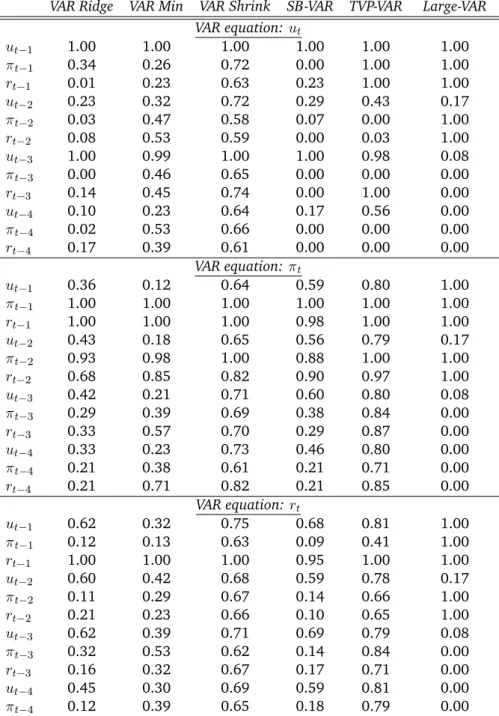
Before proceeding to the forecast evaluation of variable selection, it would be interesting first to obtain a picture of what is the output of variable selection. Since the Gibbs sampler provides a sequence of 0-1 draws from the posterior of , once we take an average of these draws we can end up with an average “probability of inclusion in the true model” for the respective VAR coefficients . Table 2 does exactly that for the six models described earlier. The table is split in three blocks pertaining to each of the three VAR equations (unemploymentut, inflation tand
interest ratert). Each row corresponds to the lags of the three variables as they appear in each
equation. Numerical entries in this table are the averages of the posterior of using the full sample 1971:Q1 - 2008:Q4. The prior on for the five trivariate VARs is theBernoulli(0:8)
discussed earlier, whilst for the Large VAR model the tighter prior discussed in subsection 3.4 applies.
Variable selection indicates that some variables should always be included, irrespective of the model specification or the priors used. These are the first own lags of each dependent variable, but also the first lag of the interest rate in the inflation equation. Moreover, inflation and interest rates two periods ago seem to affect the current level of inflation, as well as the
Table 2: Posterior means of the restriction variables jusing the full sample VAR Ridge VAR Min VAR Shrink SB-VAR TVP-VAR Large-VAR
VAR equation: ut ut 1 1.00 1.00 1.00 1.00 1.00 1.00 t 1 0.34 0.26 0.72 0.00 1.00 1.00 rt 1 0.01 0.23 0.63 0.23 1.00 1.00 ut 2 0.23 0.32 0.72 0.29 0.43 0.17 t 2 0.03 0.47 0.58 0.07 0.00 1.00 rt 2 0.08 0.53 0.59 0.00 0.03 1.00 ut 3 1.00 0.99 1.00 1.00 0.98 0.08 t 3 0.00 0.46 0.65 0.00 0.00 0.00 rt 3 0.14 0.45 0.74 0.00 1.00 0.00 ut 4 0.10 0.23 0.64 0.17 0.56 0.00 t 4 0.02 0.53 0.66 0.00 0.00 0.00 rt 4 0.17 0.39 0.61 0.00 0.00 0.00 VAR equation: t ut 1 0.36 0.12 0.64 0.59 0.80 1.00 t 1 1.00 1.00 1.00 1.00 1.00 1.00 rt 1 1.00 1.00 1.00 0.98 1.00 1.00 ut 2 0.43 0.18 0.65 0.56 0.79 0.17 t 2 0.93 0.98 1.00 0.88 1.00 1.00 rt 2 0.68 0.85 0.82 0.90 0.97 1.00 ut 3 0.42 0.21 0.71 0.60 0.80 0.08 t 3 0.29 0.39 0.69 0.38 0.84 0.00 rt 3 0.33 0.57 0.70 0.29 0.87 0.00 ut 4 0.33 0.23 0.73 0.46 0.80 0.00 t 4 0.21 0.38 0.61 0.21 0.71 0.00 rt 4 0.21 0.71 0.82 0.21 0.85 0.00 VAR equation: rt ut 1 0.62 0.32 0.75 0.68 0.81 1.00 t 1 0.12 0.13 0.63 0.09 0.41 1.00 rt 1 1.00 1.00 1.00 0.95 1.00 1.00 ut 2 0.60 0.42 0.68 0.59 0.78 0.17 t 2 0.11 0.29 0.67 0.14 0.66 1.00 rt 2 0.21 0.23 0.66 0.10 0.65 1.00 ut 3 0.62 0.39 0.71 0.69 0.79 0.08 t 3 0.32 0.53 0.62 0.14 0.84 0.00 rt 3 0.16 0.32 0.67 0.17 0.71 0.00 ut 4 0.45 0.30 0.69 0.59 0.81 0.00 t 4 0.12 0.39 0.65 0.18 0.79 0.00 rt 4 0.07 0.30 0.66 0.17 0.66 0.00
third lag of unemployment affects the current level of unemployment (but only in the small, trivariate VAR models). Lastly, unemployment in the previous quarter is more likely to affect the current level of the interest rate than past inflation.
Other than these few regularities, the posterior probabilities of inclusion of each predictor variable varies a lot between specifications. For the linear VAR model, the relatively
uninfor-mative ridge regression prior invites more restrictions from the variable selection algorithm than when the Minnesota and Normal-Jeffrey’s priors are present. This is because the last two priors already provide shrinkage of coefficients towards zero. Subsequently it is the case that shrinkage will force more (compared to an uninformative prior) the posterior of the j’s to
move towards the region of zero, so that the respective j’s are not identified and they will be drawn randomly from theirBernoulli(0:8)prior. As discussed earlier, this is not a failure of variable selection since what we care about is the combined coefficient j = j j to be zero,
whether it is because j = 0 or j = 0. An example where this effect happens is for variable
t 2 in the unemployment equation, which has only a probability of 8% of inclusion when
using the VAR Ridge model, but this probability increases to circa 50% when using the VAR Min and VAR Shrink models. Nevertheless, in these two latter models, the posterior mean of
j forj= t 2 is around 0.002, so that it finally holds that j = j j 0.
For the rest of the VAR models mixed results are present which depend on the nature of each model. Even among the two nonlinear models many differences exist. For instance,
t 1 has 0% probability of appearing in the unemployment equation of the structural breaks
VAR but 100% probability of appearing in the same equation in the time-varying VAR model. Finally, notice that more restrictions are present in the Large-VAR model since a more restricted form of the prior on is used, compared to the one used in the small models. In this Large-VAR setting the right-hand side (RHS) variables have exactly the same probability of appearing in each of the three VAR equations of interest. This is due to the simplifying assumption described in subsection 3.4 which allows computational tractability when the dimensions of the VAR grow large.
4.5 Out-of-sample iterated forecasts
In this subsection the restricted and unrestricted VAR models are evaluated out-of-sample. Tables 3 and 4 present the MAFE and RMSFE statistics over the forecast sample 1990:Q1-2008:Q4. The first column of each table shows the three variables in the vector of interest yt+h, for horizonsh = 1; :::;4. The second column of both tables presents the absolute value
of the MAFE and RMSFE, respectively, for the driftless random walk model. Consequently the remaining columns present the MAFE and RMSFE statistics from the six Bayesian four-lag VARs with and without variable selection, as a proportion of the respective MAFE and RMSFE of the random walk. For comparison the third column in each table gives the respective statistics from a parsimonious VAR(1) specification estimated with OLS.
The results suggest that all small four-lag VAR models perform better the naïve model in short-term forecasting of unemployment and inflation. The very flexible TVP-VAR provides the lowest mean prediction error (the gains are especially visible during the financial crisis sample 2007-2008), while the Large VAR being quite heavily parametrized gives only the best VAR forecasts for the interest rate. Nevertheless, none of the VAR models can beat the random walk in interest rate forecasting.
T able 3: R elative MAFE of unrestricted and restricted V ARs: unemployment, inflation and interest rate for h = 1 , 2 , 3 and 4 . R W V AR(1) V AR(4) Ridge V AR(4) Min V AR(4) Shrink SB -V AR(4) TVP -V AR(4) Large-V AR(4) MAFE OLS no VS with VS no VS with VS no VS with VS no VS with VS no VS with VS no VS with VS ut+1 0.1343 1.07 0.88 0.88 0.87 0.86 0.86 0.86 0.88 0.86 0.84 0.84 0.95 0.86 t +1 0.4882 1.18 0.91 0.88 0.90 0.88 0.88 0.89 0.90 0.90 0.83 0.83 1.24 1.21 rt+1 0.4047 1.31 1.45 1.45 1.43 1.44 1.42 1.41 1.36 1.33 1.33 1.33 1.22 1.17 ut+2 0.2163 1.14 0.94 0.92 0.93 0.93 0.92 0.91 0.94 0.86 0.83 0.84 1.03 0.90 t +2 0.8173 1.24 1.00 1.00 0.96 0.97 1.00 1.02 0.97 1.01 0.86 0.88 1.36 1.29 rt+2 0.6971 1.38 1.59 1.55 1.57 1.52 1.50 1.47 1.50 1.47 1.39 1.37 1.09 1.01 ut+2 0.2912 1.15 0.96 0.92 0.95 0.94 0.93 0.92 0.95 0.87 0.79 0.81 1.12 0.91 t +3 1.1014 1.35 1.18 1.16 1.12 1.09 1.13 1.14 1.15 1.11 0.88 0.91 1.64 1.53 rt+3 0.9532 1.45 1.74 1.64 1.70 1.60 1.55 1.51 1.63 1.46 1.47 1.41 1.06 1.03 ut+4 0.3479 1.16 0.99 0.95 0.99 0.98 0.97 0.96 0.99 0.88 0.80 0.83 1.22 0.93 t +4 1.2863 1.51 1.49 1.46 1.40 1.34 1.37 1.37 1.46 1.45 1.02 1.01 1.91 1.77 rt+4 1.1868 1.52 1.79 1.70 1.74 1.65 1.58 1.54 1.68 1.49 1.49 1.44 1.10 1.04 Note: The seco nd column shows the absol ute MAFE of the Random W alk (R W). The remaining columns report MAFEs of ea ch V AR model relative to th e MAFE of the R W . No VS/ with VS indicates if variab le selection is present or n ot. T able 4: R elative RMSFE of unrestricted and restricted V ARs: unemployment, inflation and interest rate for h = 1 , 2 , 3 and 4 . R W V AR(1) V AR(4) Ridge V AR(4) Min V AR(4) Shrink SB -V AR(4) TVP -V AR(4) Large-V AR(4) MAFE OLS no VS with VS no VS with VS no VS with VS no VS with VS no VS with VS no VS with VS ut+1 0.1712 1.07 0.85 0.84 0.84 0.84 0.83 0.83 0.85 0.85 0.79 0.80 0.92 0.86 t +1 0.6828 1.10 0.85 0.84 0.85 0.86 0.87 0.88 0.85 0.89 0.79 0.80 1.13 1.11 rt+1 0.6378 1.16 1.24 1.25 1.23 1.23 1.24 1.23 1.17 1.23 1.16 1.18 1.07 1.04 ut+2 0.2933 1.04 0.84 0.81 0.83 0.82 0.82 0.81 0.83 0.81 0.75 0.77 0.91 0.84 t +2 1.1157 1.22 0.95 0.96 0.93 0.94 0.97 0.98 0.93 1.03 0.80 0.81 1.26 1.19 rt+2 1.0278 1.23 1.37 1.33 1.34 1.32 1.30 1.29 1.29 1.28 1.24 1.24 1.00 0.93 ut+2 0.4047 1.00 0.85 0.81 0.84 0.83 0.82 0.81 0.84 0.81 0.73 0.76 0.99 0.84 t +3 1.4596 1.37 1.16 1.16 1.12 1.10 1.12 1.13 1.13 1.08 0.89 0.91 1.55 1.47 rt+3 1.3441 1.28 1.47 1.40 1.43 1.37 1.34 1.32 1.39 1.29 1.30 1.30 1.00 0.99 ut+4 0.4986 0.96 0.82 0.79 0.82 0.81 0.80 0.79 0.82 0.79 0.70 0.73 1.05 0.83 t +4 1.7036 1.54 1.44 1.42 1.37 1.32 1.33 1.33 1.41 1.41 1.03 1.03 1.83 1.72 rt+4 1.6406 1.31 1.49 1.43 1.46 1.40 1.36 1.33 1.41 1.30 1.31 1.28 1.03 1.02 Note: The seco nd column shows the absol ute RMSFE of the Random W alk (R W). The remaining columns report RMSFEs of each V AR model relative to the RMSFE of the R W . No V S/ with VS indicates if va riable selection is present o r not.
In terms evaluating variable selection, the unrestricted VAR(4) model with ridge regres-sion prior (which in this paper is defined to be uninformative, as if using a VAR(4) estimated with least squares) is better at all horizons than the unrestricted, more parsimonious VAR(1) in forecasting unemployment and inflation. In that respect, good performance of the variable selection is translated into expecting substantial restrictions of the VAR(4) Ridge model coeffi-cients only in the interest rate equation since from the VAR(1) it is obvious that using one lag in this equation is always better. At the same time less restrictions are expected in the coeffi-cients in the unemployment and interest rate equation, since the VAR(4) is already doing much better than the VAR(1) for these two equations. Table 2 provided an idea of the restrictions that actually hold in each model, however notice that in a recursive forecasting exercise the posterior probabilities are estimated in real-time as new data become available, so they will not be constant during the forecast evaluation sample.
In fact, variable selection in the VAR(4) Ridge model does improve forecasts of all three variables, especially at longer horizons. For the VAR(4) Min and VAR(4) Shrink (these two models already have shrinkage priors) variable selection only improves the interest rate fore-cast while there is usually a 1% gain/loss in MAFE or RMSFE, but this is so small that might also be attributed to sampling and rounding error. The main result is that none of the three unrestricted linear VARs with four lags is forecasting interest rates as the VAR(1) estimated with OLS does, something that is consistently accounted for when adding variable selection9.
The gains from variable selection for forecasting all three variables of interest are more clear as the model size increases. As forecasting results for the 13-variable Large VAR suggest, when the model dimensions increase, variable selection really helps to prevent overfitting. Although the Minnesota shrinkage parameter is not set optimally, this improvement when using variable selection is robust for a large grid of values of (see the discussion in subsection 4.1).
The story behind the structural breaks model SB-VAR(4) is different. There, the gains are quite impressive for longer horizons, but closer examination shows that these are linked only indirectly to variable selection. Estimation of the unrestricted SB-VAR(4) model with maximum number ofpossiblebreaks equal to 3, indicates that there are actually no breaks10. When the SB-VAR(4) model is estimated with variable selection, a break is found (using the full sample) in 2004Q1. This is actually the exact reason why variable selection does much better in mean prediction with the structural breaks model. By restricting the parameter space, a structural break is found that is not otherwise identified when all 39 mean VAR coefficients are unrestricted.
In the TVP-VAR model with Minnesota prior, which is the best performing among all VAR models, variable selection helps improve the MAFE of the interest rate in longer horizons. Nevertheless, in this case variable selection increases the absolute and squared forecast error of unemployment and inflation at horizons two to four quarters. Subsequently, the shrinkage
9Here we can observe that although variable selection improves forecasts of interest rate from the linear VAR(4),
these are never as good as the VAR(1)-OLS forecasts. This is due to the fact that our prior expection is that 20% of the parameters should be restricted ( 0j= 0= 0:8). Subsequently there might be benefit from setting 0j<<0:8
but only if jis a coefficient in the interest rate equation; see also the discussion in the next subsection.
10Notice that although no breaks are estimated, the SB-VAR(4) forecasts are not the same as the VAR(4) Min
forecasts (these two models have identical Minnesota priors). The reason is computational, but explaining why is beyond the scope of this paper. The reader is advised to consult Bauwens, Koop, Korobilis and Rombouts (2011).
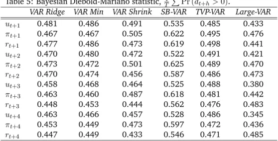
prior in this case is sufficient to guarantee optimal mean forecasts, and variable selection is not necessary. Although this observation might be correct for the expected risk of mean forecasts, the Bayesian Diebold-Mariano (BDM) statistic given in equation (22) reveals that there is the case that variable selection provides overall superior predictive ability.
The BDM statistic, which is based on the time series of differences between the squared forecast errors of the restricted and the unrestricted models, is presented in Table 5. A value less than 0.5 shows the probability that the restricted model has better forecasting ability overall compared to the unrestricted model. Table 5 reveals that this is the case for all models apart from the structural breaks VAR. That is because in this model we saw that variable selection indicates one break, while in the unrestricted model no break is found. Thus forecasts from the restricted model with one break have larger variance because all the VAR coefficients in the second regime are estimated using only 19 observations (the break date is 2004Q1). Since the BDM statistic is based on all simulated draws from the posterior predictive densities, parameter uncertainty is included in the evaluation of the quantity Pr (dt+h>0). Thus, this
fact explains why the unrestricted no-break model does better overall than the restricted model with one break, despite the fact that the MAFE and RMSFE results suggest otherwise. Finally, in Table 5 we can observe again that as the forecast horizon increases the gains from using variable selection also increase.
Table 5: Bayesian Diebold-Mariano statistic, T1 PPr (dt+h >0).
VAR Ridge VAR Min VAR Shrink SB-VAR TVP-VAR Large-VAR
ut+1 0.481 0.486 0.491 0.535 0.485 0.433 t+1 0.467 0.467 0.505 0.622 0.495 0.476 rt+1 0.477 0.486 0.473 0.619 0.498 0.441 ut+2 0.470 0.480 0.472 0.522 0.491 0.421 t+2 0.473 0.472 0.501 0.625 0.489 0.470 rt+2 0.470 0.474 0.456 0.587 0.486 0.473 ut+3 0.458 0.468 0.464 0.525 0.488 0.380 t+3 0.463 0.460 0.487 0.618 0.481 0.442 rt+3 0.448 0.453 0.444 0.562 0.476 0.483 ut+4 0.463 0.466 0.457 0.528 0.486 0.345 t+4 0.453 0.449 0.473 0.597 0.472 0.436 rt+4 0.447 0.449 0.433 0.546 0.471 0.485
Note: The Table shows the average values of the statistic Pr(dt+h>0) wheredt+h are the time series of differences between the squared
forecast errors from the restricted and unrestricted models; see also equation (22) in the text.
4.6 Sensitivity analysis: Direct forecasts, and expected number of restrictions
In many cases, iterated, multi-step ahead VAR forecasts might not be satisfactory. This is particularly true when the model is misspecified (Marcellino, Stock and Watson, 2006), in which case econometricians estimate a direct VAR using information up to timet to directly predictyt+h, i.e. the model
yt+h =Bxt+"t:
Using the above VAR equation, the researcher can use directly the available informationxT to
predictors for which forecasts are not available to the econometrician (and hence iterating the VARh-steps ahead is not possible).
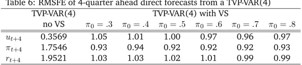
This case is examined analytically in Korobilis (2008) using the SSVS algorithm in large linear VARs with hundreds of predictors. Here I provide results for 4-steps ahead forecasting using the TVP-VAR(4) in the context of a “sensitivity analysis” with varying degree of prior expected number of restrictions. Restrictions in the VAR models with variable selection can be imposed through the prior hyperparameter 0j of the Bernoulli density in equation (6).
Table 6 presents the RMSFE from the unrestricted TVP-VAR(4) in the second column, and the RMSFE of the restricted TVP-VAR(4) with 0j = 0 for all j = 1; :::; n, relative to that of the
unrestricted model. The case 0 = 0:8is the one examined previously in the small VARs (but it
was relaxed in the Large VAR model) and implies the expectation that 20% of the coefficients should be restricted a priori. Other values shown in this Table can be interpreted in a similar way. The optimal forecasts from the restricted model are obtained when 0 is 0.7, where
gains of up to 8% in forecasting inflation are attained. When more and more restrictions are imposed, the RMSFE are monotonically increasing, suggesting that there is a risk attached to imposing strong prior beliefs in such a small model. For 0 >0:7 the RMSFE also increases,
where the limit 0 = 1implies the unrestricted model (where all relative RMSFEs are equal to
1.00).
Table 6: RMSFE of 4-quarter ahead direct forecasts from a TVP-VAR(4)
TVP-VAR(4) TVP-VAR(4) with VS
no VS 0 =:3 0 =:4 0 =:5 0 =:6 0 =:7 0=:8
ut+4 0.3569 1.05 1.01 1.00 0.97 0.96 0.97
t+4 1.7546 0.93 0.94 0.92 0.92 0.92 0.93
rt+4 1.9521 1.03 1.03 1.02 1.01 0.99 0.99
Note: The second column presents the RMSFE of the unrestricted TVP-VAR(4) model. The next columns present the RMSFEs of the restricted
model (relative to that of the unrestricted TVP-VAR(4)) for different prior expected number of restrictions on .
Although for other direct VAR models and forecast horizons results are mixed as to whether variable selection improves forecasting over the unrestricted model, it is always the case that for small VAR models the RSMFE is a quadratic function of 0. Consequently, choice of 0
should not pose a challenge for the applied researcher as soon as the choice of expected re-strictions is chosen reasonably, i.e. it is tied to the dimension of the VAR model considered. For instance, in subsection 3.4 an empirical method for tuning the prior expected number of restrictions as the dimension of the VAR increases was introduced. Moreover, if there are actu-ally practical difficulties in selecting a value for 0, full Bayes methods can also be used. That
means that a hyperpior distribution is placed on 0 (or even 0j for j = 1; :::; n), so that this
hyperparameter is estimated from the data and hence it will also vary with the sample size considered.
5
Concluding remarks
Vector autoregressive models have been used extensively over the past for the purpose of macroeconomic forecasting, since they have the ability to fit the observed data better than competing theoretical and large-scale structural macroeconometric models. This paper shows
that Bayesian variable selection methods can be used to find restrictions based on the evidence in the data with positive implications in preserving parsimony. It was argued that these types of restrictions are important for long-horizon forecasts as well as forecasts from large VAR systems. Specifically, variable selection i) dominates forecast from VAR models with uninfor-mative priors; ii) competes favourably to shrinkage estimation; and iii) provides more benefits in forecasting as the model size increases.
References
Ba´nbura, M., Giannone, D. and Reichlin, L. (2010). Large Bayesian vector auto regressions. Journal of Applied Econometrics, 25, 71-92.
Barbieri, M. M., and J. O. Berger. (2004). Optimal predictive model selection. The Annals of Statistics, 32, 870-897.
Bauwens, L., Koop, G., Korobilis, D., and J. Rombouts. (2011). A comparison of forecast-ing procedures for macroeconomic series: The contribution of structural break models. CIRANO Working Papers 2011s-13, CIRANO.
Canova, F. (1993). Modelling and forecasting exchange rates using a Bayesian time varying coefficient model. Journal of Economic Dynamics and Control,17, 233-262.
Canova, F., and L. Gambetti. (2009). Structural changes in the US economy: Is there a role for monetary policy? Journal of Economic Dynamics and Control, 33, 477-490.
Carter, C., and R. Kohn (1994). On Gibbs sampling for state space models. Biometrika, 81, 541-553.
Chan, J. C. C., Koop, G., Leon-Gonzalez, R., and Strachan, R. W. (2010). Time-varying di-mension models. ANU School of Economics Working Papers 2010-523.
Chib, S. (1996). Calculating posterior distributions and modal estimates in Markov mixture models. Journal of Econometrics, 75, 79-98.
Chipman, H., George, E. I., and R.E. McCulloch. (2001). The practical implementation of Bayesian model selection. In P. Lahiri (Ed.), Model Selection, (pp. 67-116). IMS Lecture Notes – Monograph Series, vol. 38.
Cogley, T., Morozov, S., and T. Sargent. (2005). Bayesian fan charts for U.K. inflation: Fore-casting and sources of uncertainty in an evolving monetary system. Journal of Economic Dynamics and Control, 29, 1893-1925.
Cogley, T., and T. Sargent. (2002). Evolving post-World War II inflation dynamics. NBER Macroeconomics Annual, 16, 331-388.
Clark, T. E., and M. W. McCracken. (2010). Averaging forecasts from VARs with uncertain instabilities. Journal of Applied Econometrics, 25, 5-29.
D’Agostino, A., Gambetti, L., and D. Giannone. (2009). Macroeconomic forecasting and structural change. ECARES Working Paper 2009-020.
Diebold, F. X. and R. S. Mariano. (1995). Comparing predictive accuracy. Journal of Business and Economic Statistics, 13, 253-263.
Doan, T., R. Litterman, and C. A. Sims. (1984). Forecasting and conditional projection using realistic prior distributions. Econometric Reviews, 3, 1-100.
Garratt, A., Koop, G., Mise, E. & S. P. Vahey (2009). Real-time prediction with U.K. monetary aggregates in the presence of model uncertainty. Journal of Business and Economic Statistics, 27, 480-491.
George, E. I., Sun, D. and S. Ni. (2008). Bayesian stochastic search for VAR model restrictions. Journal of Econometrics, 142, 553-580.
Groen, J., Paap, R., and F. Ravazzolo. (2009). Real-time inflation forecasting in a changing world. Unpublished manuscript.
Jochmann, M., Koop, G., and R.W. Strachan. (2010). Bayesian forecasting using stochastic search variable selection in a VAR subject to breaks. International Journal of Forecasting, 26, 326-347.
Kohn, R., Smith, M., and D. Chan. (2001). Nonparametric regression using linear combina-tions of basis funccombina-tions. Statistics and Computing, 11, 313-322.
Koop, G., and D. Korobilis. (2009a). Bayesian Multivariate time series methods for empirical macroeconomics. Foundations and Trends in Econometrics, 3, 267-358.
Koop, G., and D. Korobilis. (2009b). Forecasting inflation using dynamic model averaging. RCEA Working Paper 34-09.
Koop, G., Leon-Gonzalez, R., and R. Strachan. (2009). On the evolution of the monetary policy transmission mechanism. Journal of Economic Dynamics and Control, 33, 997-1017.
Koop, G., and S. M. Potter. (2007). Estimation and forecasting in models with multiple breaks. The Review of Economics and Statistics, 74, 763-789.
Korobilis, D. (2008). Forecasting in vector autoregressions with many predictors. Advances in Econometrics, 23, 403-431.
Korobilis, D. (2011). Hierarchical shrinkage priors for dynamic regressions with many pre-dictors. Unpublished manuscript.
Kuo, L., and B. Mallick. (1997). Variable selection for regression models. Shankya: The Indian Journal of Statistics, 60 (Series B), 65-81.
Liang, F., Paulo, R., Molina, G., Clyde, M. A. and Berger, J. O. (2008). Mixtures of g-priors for Bayesian Variable Selection. Journal of the American Statistical Association, 103, 410-423.