Convergent Projective Non-negative Matrix Factorization
Lirui Hu1,2,3, Jianguo Wu1,3 and Lei Wang1,31 Key Laboratory of Intelligent Computing and Signal Processing of Ministry of Education, Anhui University Hefei, 230039, China
2
School of Computer Science and Technology, Nantong University Nantong, 226019, China
3
School of Computer Science and Technology, Anhui University Hefei, 230039, China
Abstract
In order to solve the problem of algorithm convergence in projective non-negative matrix factorization (P-NMF), a method, called convergent projective non-negative matrix factorization (CP-NMF), is proposed. In CP-NMF, an objective function of Frobenius norm is defined. The Taylor series expansion and the Newton iteration formula of solving root are used. An iterative algorithm for basis matrix is derived, and a proof of algorithm convergence is provided. Experimental results show that the convergence speed of the algorithm is higher, however it is affected by the initial value of the basis matrix; relative to non-negative matrix factorization (NMF), the orthogonality and the sparseness of the basis matrix are better, however the reconstructed results of data show that the basis matrix is still approximately orthogonal; in face recognition, there is higher recognition accuracy. The method for CP-NMF is effective.
Keywords: Non-negative Matrix Factorization, Projective, Convergence, Face Recognition.
1. Introduction
According to the point of view which perception of the whole is based on perception of its parts, a data technology, called non-negative matrix factorization (NMF)
WH
X
»
[1], was constructed. The method had revealed the essence of describing data, and it had been widely applied to the fields of data dimension reduction, image analysis, pattern recognition [1, 2], text mining, spectral data analysis [3], and so on. NMF is a current research focus.Projective non-negative matrix factorization (P-NMF)
X
WW
X
»
T [4] was proposed based on NMF. Since it was constructed from the projection angle, the basis matrixW
was only computed in the algorithm for P-NMF. The computational complexity was lower for one iteration step for P-NMF, as only one matrix had to be computed instead of two for NMF. On the basis of optimization rule2 0
2
1
min
arg
F T W³X
-
WW
X
, the basis matrix
W
for P-NMF was forced to tend to be orthogonal. So, the orthogonality and the sparseness of the basis matrix were better in NMF than in NMF, and then the method for P-NMF was more beneficial to the applications of data dimension reduction, pattern recognition, and so on. However, the proof of algorithm convergence was not given in the paper [4]. Now, we use the objective function)
0
,
0
(
2
1
2³
³
-=
X
WW
X
W
X
F
F T and the iterative formula ij T T ij T T ij T ij ijW
WW
XX
W
XX
WW
W
XX
W
W
)
(
)
(
)
(
2
+
=
(1)in the paper [4] to do an experiment. In Eq. (1),
X
consists of the first five images of each person in the ORL facial image database, a total of 200 data. We set the rank of the basis matrix
W
80 and initialize it with non-negative data. In order to reduce the amount of computation and improve the speed of operation, each image is reduced to a quarter of the original. After 10000 iteration steps, we will see that the varied curve of the objective function values versus iteration steps is severely concussive, and the algorithm does not converge. Here, in order to make the graphics clearly seen, we give the varied curve of objective function values versus iteration steps after 100 iteration steps, and the curve is shown in Fig. 1.0 20 40 60 80 100 0 2 4 6 8x 10 11 Iteration steps O b je c ti v e f u n c ti o n v a lu e
In order to solve the problem of algorithm convergence in P-NMF, a method is proposed based on P-NMF
X
WW
X
»
T in this paper. We call it convergent projective non-negative matrix factorization (CP-NMF). In this method, another iterative algorithm for the basis matrixW
is constructed, and strict proof of algorithm convergence is provided, and the convergence speed of the algorithm is higher. Like P-NMF, the orthogonality and the sparseness of the basis matrix are still better in CP-NMF. We compare this method with the methods of NMF, LNMF [5], and NMFOS [6], and the experimental results show that this method has higher recognition accuracy in face recognition.The rest of this paper is organized as follows. In Section 2, our method is introduced in detail. Firstly, an iterative formula for basis matrix
W
is derived strictly based onX
WW
X
»
T . Secondly, a proof of algorithm convergence is provided. Finally, the algorithm steps are given. In Section 3, the convergence of the algorithm is validated by numerical experiments, and it is emphasized that the convergence speed of the algorithm is affected by the initial value of the basis matrixW
and the basis matrixW
is still approximately orthogonal. Moreover, by numerical experiments in face recognition, we compare this method with NMF and some extended methods in Section 4, and explain the effectiveness of the method. In the end, conclusions are drawn in Section 5.2. Convergent Projective Non-negative Matrix
Factorization (CP-NMF)
We consider an objective function [4] 2
2
1
F TX
WW
X
F
=
-
(2) whereX
³
0
,
W
³
0
.
Obviously,F
is a function defined in P-NMF. We may minimizeF
to getW
.2.1 The Iterative Rule for Basis Matrix
W
For any element
w
ab ofW
, letab
w
F
stand for the part ofF
relevant tow
ab in Eq. (2). So, writingw
instead of abw
in the expression ofab
w
F
, we may get a function).
(
w
F
ab
w Obviously, the first order derivative of
)
(
w
F
ab
w at
w
ab is the first order partial derivative ofF
with respect tow
ab. That isab ij ij T ij ab ab w
w
X
WW
X
w
F
w
F
ab
-
=
=
å
2 ']
)
(
[
2
1
(
)
(
ab ij T ij ij T ijw
X
WW
X
WW
X
-=
å
(
(
)
)
(
)
ab k kj ik T ij ij T ijw
X
WW
X
WW
X
+
-=
å
å
)
)
(
(
)
)
(
(
)
)
(
)(
)
(
(
å
å
-
+
=
k kj ab ik T ij ij T ijX
w
WW
X
WW
X
)
)
(
)(
)
(
(
å
å
å
-
+
=
k kj ab l kl il ij ij T ijX
w
W
W
X
WW
X
)
)
(
)(
)
(
(
å
å
-
+
=
k kj ab kb ib ij ij T ijX
w
W
W
X
WW
X
å
åå
-
+
=
k kj ab kb ib j i ij T ijX
w
W
W
X
WW
X
(
)
)
(
(
)
)
(
å
å
+
+
-=
j k kj ab kb ab aj T ajX
w
W
W
X
WW
X
(
)
)(
(
)
)
[(
]
)
)
(
)(
)
(
(
å
å
¹
+
-a i k kj ab kb ib ij T ijX
w
W
W
X
WW
X
å
å
¹+
+
-=
j k a kj ab kb ab aj T ajX
w
W
W
X
WW
X
(
)
)(
(
)
[(
]
)
)
(
(
)
)
(
å
¹+
-+
a i aj ib ij T ij aj ab ab abX
W
X
WW
X
X
w
W
W
å
å
¹+
+
+
-=
j k a aj ab kj kb aj T ajWW
X
W
X
W
X
X
(
)
)(
2
)
[(
-+
-å
i aj ib ij T ijWW
X
W
X
X
(
)
)
(
]
)
)
(
(
aj ab aj T ajWW
X
W
X
X
+
-å
å
¹+
+
+
-=
j k a aj ab kj kb aj T ajWW
X
W
X
W
X
X
(
)
)(
)
[(
å
-
+
i aj ib ij T ijWW
X
W
X
X
(
)
)
(
]+
+
-=
å
j bj T aj T ajWW
X
W
X
X
(
)
)(
)
[(
å
å
-
+
i aj ib ij T i aj ib ijW
X
WW
X
W
X
X
)
(
)
(
]å
å
+
-=
j bj T aj T j bj T ajW
X
WW
X
W
X
X
(
)
(
)
(
)
å
å
+
-j bj T T aj j bj T ajW
X
X
W
WW
X
X
(
)
(
)
-+
-=
T T ab ab TW
XX
WW
W
XX
)
(
)
(
ab T T ab TW
WW
XX
W
XX
)
(
)
(
+
+
+
-=
T T ab ab TW
XX
WW
W
XX
)
(
)
(
2
ab T TW
WW
XX
)
(
. (3)Similarly, in order to get the second order derivative of
)
(
w
F
ab w atw
ab,we can get ab ab Tw
W
XX
-
(
2
(
)
)
aa TXX
)
(
2
-=
,+
=
aa T T ab ab T TXX
WW
w
W
XX
WW
)
(
)
(
+
bb T TW
XX
W
)
(
(
XX
TW
)
abW
ab , and+
=
aa T T ab ab T TXX
WW
w
W
WW
XX
)
(
)
(
+
ab ab TW
W
XX
)
(
å
k kb aa TW
XX
2)
(
.So, the second order derivative of
F
(
w
)
ab w at
w
ab is ab ab T T ab ab T ab ww
W
XX
WW
w
W
XX
w
F
ab
+
-
=
(
2
(
)
)
(
)
)
(
'' ab ab T Tw
W
WW
XX
+
(
)
bb T T aa T T aa TW
XX
W
XX
WW
XX
)
2
(
)
(
)
(
2
+
+
-=
å
+
+
k kb aa T ab ab TW
XX
W
W
XX
)
(
)
2(
2
. (4)Similarly, in order to get the third order derivative of
)
(
w
F
ab w atw
ab,we can get0
)
(
=
ab aa Tw
XX
, ab aa T Tw
XX
WW
(
)
ab T ab aa TW
XX
W
XX
)
(
)
(
+
=
, ab bb T Tw
W
XX
W
(
)
ab TW
XX
)
(
2
=
, ab ab ab Tw
W
W
XX
(
)
ab aa T ab TW
XX
W
XX
)
(
)
(
+
=
, and ab aa T ab k kb aa TW
XX
w
W
XX
)
(
2
)
)
((
2=
å
. So, the third order derivative ofF
(
w
)
ab w at
w
ab is ab aa T ab T ab ww
XX
W
XX
W
F
ab(
)
6
(
)
6
(
)
'' '=
+
. (5) Similarly, in order to get the fourth order derivative of)
(
w
F
ab w atw
ab,we can get aa T ab k kb ak T ab ab TXX
w
W
XX
w
W
XX
)
(
)
)
(
(
)
(
=
=
å
and aa T ab ab aa TXX
w
W
XX
)
(
)
)
((
=
. So, the fourth order derivative ofF
(
w
)
ab w at
w
ab is aa T ab ww
XX
F
ab(
)
12
(
)
) 4 (=
, (6) and other order derivatives ofF
(
w
)
ab w with respect to
w
are0
)
(
) (=
w
F
wabn (7) where n³5.Thus, the Taylor series expansion of
F
(
w
)
ab w at
w
ab is+
-+
=
(
)
(
)(
)
)
(
w ab ' ab ab ww
F
w
F
w
w
w
F
ab w ab ab+
-+
-
2 ''' 3 '')
)(
(
6
1
)
)(
(
2
1
ab ab w ab abw
w
F
w
w
w
w
F
ab ab w 4 ) 4 ()
)(
(
24
1
ab ab ww
w
w
F
ab-
. (8)Meantime, to emphasize time of
w
ab in numerical calculation, we writew
ab(t) instead ofw
ab in the brackets ofF
(
w
)
ab w . So, equation+
-+
=
(
)
(
)(
)
)
(
() ' () (t) ab t ab t ab w ww
F
w
F
w
w
w
F
ab w ab ab 3 ) ( ) ( '' ' 2 ) ( ) ( '')
)(
(
6
1
)
)(
(
2
1
t ab t ab w t ab t abw
w
F
w
w
w
w
F
ab ab w-
+
-4 ) ( ) ( ) 4 ()
)(
(
24
1
t ab t ab ww
w
w
F
ab-+
(9) is gotten from Eq. (8).+
-+
=
(
)
(
)(
)
)
,
(
() () ' () ab(t) t ab w t ab w t ab ww
w
F
w
F
w
w
w
G
ab ab ab+
+
) ()
(
)
(
[
2
1
t ab ab T T ab T Tw
W
WW
XX
W
XX
WW
+
+
+
(
)
(t)2
(
)
2 ab ab ab T ab bb T Tw
W
W
XX
W
W
XX
W
+
-å
2 ) ( ) ( 2)
](
)
)
((
t ab t ab ab k kb aa Tw
w
w
W
W
XX
4 ) ( ) ( ) 4 ( 3 ) ( ) ( '' ')
)(
(
24
1
)
)(
(
6
1
t ab t ab w t ab t ab ww
w
w
F
w
w
w
F
ab ab-
+
-
. (10)Theorem 1.
G
wab(
w
,
w
ab(t))
is an auxiliary function for)
(
w
F
ab w . Proof:G
(
w
,
w
())
F
(
w
)
ab ab w t ab w=
is obvious whenw
w
ab(t)=
. We need show thatG
(
w
,
w
())
F
(
w
)
ab ab w t ab w
³
whenw
tw
ab¹
) ( . BecauseW
³
0
,
X
³
0
,
å
=
k t kb ak T T ab T TW
XX
WW
W
XX
WW
())
(
)
(
) ()
(
aa abt T TW
XX
WW
³
andå
=
k t kb ak T T ab T TW
WW
XX
W
WW
XX
)
(
)
()(
) ()
(
aa abt T TW
WW
XX
³
) ()
(
aa abt T TW
XX
WW
=
. So, ab T T ab T TW
WW
XX
W
XX
WW
)
(
)
(
+
) ()
(
2
t ab aa T TW
XX
WW
³
. WhenW
ab(t)>
0
,
) ()
(
)
(
t ab ab T T ab T TW
W
WW
XX
W
XX
WW
+
aa T TXX
WW
)
(
2
³
. In fact, () (t).
ab t ab abW
w
W
=
=
So+
+
) ()
(
)
(
t ab ab T T ab T Tw
W
WW
XX
W
XX
WW
+
+
) ( 2)
(
2
)
(
t ab ab ab T ab bb T Tw
W
W
XX
W
W
XX
W
) ( 2)
)
((
t ab ab k kb aa Tw
W
W
XX
å
bb T T aa T T aa TW
XX
W
XX
WW
XX
)
2
(
)
(
)
(
2
+
+
-³
å
+
+
k kb aa T ab ab TW
XX
W
W
XX
)
(
)
2(
2
)
(
() '' t ab ww
F
ab=
, and then)
(
)
,
(
w
w
()F
w
G
ab ab w t ab w³
.Thus,
G
wab(
w
,
w
ab(t))
is an auxiliary function for)
(
w
F
wab according to the definition 1 of reference [7]. Theorem 2.F
(
w
)
ab
w is nonincreasing under the update
)
,
(
min
arg
() ) 1 ( t ab w w t abG
w
w
w
ab=
+ Proof: Because)
,
(
)
,
(
)
(
( 1) ( 1) () () ab(t) t ab w t ab t ab w t ab ww
G
w
w
G
w
w
F
ab ab ab£
£
+ +)
(
ab(t) ww
F
ab=
,)
(
w
F
ab w is nonincreasing.Using the definition of auxiliary function and Theorem 2, we can get the local minimum of
F
(
w
)
ab
w if only the local minimum of
G
wab(
w
,
w
ab(t))
is gotten. To get a local minimum ofF
(
w
)
ab
w , we may calculate the first order derivative of
G
wab(
w
,
w
ab(t))
with respect tow
, and have+
=
(
)
)
,
(
() ' () ' t ab w t ab ww
w
F
w
G
ab ab+
+
) ()
(
)
(
[
t ab ab T T ab T Tw
W
WW
XX
W
XX
WW
+
+
) ( 2)
(
2
)
(
t ab ab ab T ab bb T Tw
W
W
XX
W
W
XX
W
+
-å
)
](
)
)
((
) ( ) ( 2 t ab t ab ab k kb aa Tw
w
w
W
W
XX
3 ) ( ) ( ) 4 ( 2 ) ( ) ( '' ')
)(
(
6
1
)
)(
(
2
1
t ab t ab w t ab t ab ww
w
w
F
w
w
w
F
ab ab-
+
-
. (11) In order to get the root of the equation=
)
,
(
( ) ' t ab ww
w
G
ab 0, (12)we have known that the function
G
w'ab(
w
,
w
ab(t))
is a Taylor series expansion with respect tow
from Eq. (11), and then may use the Newton iteration formula of solving root to get the root of Eq. (12). That is)
,
(
)
,
(
) ( ) ( '' ) ( ) ( ' ) ( t ab t ab w t ab t ab w t abw
w
G
w
w
G
w
w
ab ab-=
. (13) In Eq. (13),)
(
)
,
(
() () ' () ' t ab w t ab t ab ww
w
F
w
G
ab ab=
and+
=
() ) ( ) ( ''(
)
)
,
(
t ab ab T T t ab t ab ww
W
XX
WW
w
w
G
ab+
+
) ()
(
)
(
t ab ab bb T T ab T Tw
W
W
XX
W
W
WW
XX
) ( 2 2)
)
((
)
(
2
t ab ab k kb aa T ab ab Tw
W
W
XX
W
W
XX
+
å
.Using Eq. (3), we simplify the Eq. (13) to
D
M
w
=
(14) where+
+
=
T T bb ab ab TW
W
XX
W
W
XX
M
[
2
(
)
(
)
) ( 2 2]
)
)
((
)
(
2
ab abt k kb aa T ab ab Tw
W
W
XX
W
W
XX
+
å
(15) and+
+
=
T T ab ab T TW
WW
XX
W
XX
WW
D
(
)
(
)
+
+
2)
(
2
)
(
W
TXX
TW
bbW
abXX
TW
abW
ab ab k kb aa TW
W
XX
)
)
((
å
2 . (16) So, the iterative rule ofw
ab isD
M
w
ab(t+1)=
. (17)Because the Newton iteration formula of solving root is convergent, we may use this iterative rule Eq. (17) and make the auxiliary function
G
w(
w
,
w
ab(t))
ab local
minimum, and thus make the objective function
F
(
w
)
ab
w local minimum. If all elements of
W
are updated by Eq. (17), the local minimum of the objective functionF
may be gotten.Therefore, the algorithm converges.The Eq. (17) is the iterative update rule for the basis matrix
W
.2.2 Algorithm Steps
Using Eq. (17), we may get an algorithm to compute the basis matrix
W
. As follows:Step1: initialize
W
andX
with non-negative data;Step2: update
W
by Eq. (15), Eq. (16) and Eq. (17);Step3: repeat step2 until algorithm converges. n
W
andW
n+1 are respectively used to denote the nthandn+1th iterative result of the basis matrix
W
. The condition of algorithm convergence is that there is0
,
2 1-
<
"
>
+ n Fe
e
nW
W
(18)for an arbitrarily small positive number
e
. In inequality (18), F stands for Frobenius norm.3. Experiments and Analysis
In the following experiments,
X
consists of the first five images of each person in the ORL facial image database, a total of 200 data. We set the rank of the basis matrixW
80. In order to reduce the amount of computation and speed up the operating speed, every image is reduced to half.
3.1 Algorithm Convergence
In order to make the process of algorithm convergence seen more clearly in the graph, we set the larger
e
0.001, and randomly initializeW
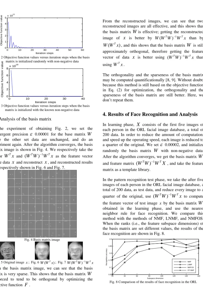
with non-negative data. The set precision of algorithm convergence is obtained after 60 iterations. In this case, the varied curve of the objective function values versus iteration steps is shown in Fig. 2. We can see that the convergence speed of the algorithm is higher. In addition, we initializeW
with the first two images of each person in the ORL, and do an experiment again. The same precision of algorithm convergence is obtained after 39 iterations. The varied curve is shown in Fig. 3. We can see faster convergence of the algorithm. This shows the initial value of the basis matrix affects the convergence speed of the algorithm. The reason is that the convergence speed of Newton iteration formula is dependent on initial value, and the initial value is close to the root convergence faster.0 10 20 30 40 50 60 0 1 2 3 4 5x 10 11 Iteration steps O b je c ti v e f u n c ti o n v a lu e
Fig. 2 Objective function values versus iteration steps when the basis matrix is initialized randomly with non-negative data
0 10 20 30 40 0 2 4 6 8x 10 19 Iteration steps O b je c ti v e f u n c ti o n v a lu e
Fig. 3 Objective function values versus iteration steps when the basis matrix is initialized with the known non-negative data
3.2 Analysis of the basis matrix
In the experiment of obtaining Fig. 2, we set the convergent precision
e
0.00001 for the base matrixW
while the other set data are unchanged, and do an experiment again. After the algorithm converges, the basis matrix image is shown in Fig. 4. We respectively take the vectorW
Tx
and(
W
TW
)
-1W
Tx
as the feature vector of the datax
and reconstructx
, and reconstructed results are respectively shown in Fig. 6 and Fig. 7.Fig. 4 Basis matrix image
Fig. 5 Original image x; Fig. 6 W(WTx); Fig. 7
x W W W W T 1 T ) (
-From the basis matrix image, we can see that the basis matrix is very sparse. This shows that the basis matrix
W
is forced to tend to be orthogonal by optimizing the objective function
F
.From the reconstructed images, we can see that two reconstructed images are all effective, and this shows that the basis matrix
W
is effective; getting the reconstructed image ofx
is better by W(WTW)-1WTx than by)
(
W
x
W
T , and this shows that the basis matrixW
is still approximately orthogonal, therefore getting the feature vector of datax
is better using (WTW)-1WTx than usingW
Tx
.The orthogonality and the sparseness of the basis matrix may be computed quantificationally [8, 9]. Without doubt, because this method is still based on the objective function in Eq. (2) for optimization, the orthogonality and the sparseness of the basis matrix are still better. Here, we don’t repeat them.
4. Results of Face Recognition and Analysis
In learning phase,
X
consists of the first five images of each person in the ORL facial image database, a total of 200 data. In order to reduce the amount of computation, and speed up the operating speed, each image is reduced to a quarter of the original. We sete
0.00002, and initialize randomly the basis matrixW
with non-negative data. After the algorithm converges, we get the basis matrixW
and feature matrix
(
W
TW
)
-1W
TX
, and take the feature matrix as a template library.In the pattern recognition test phase, we take the after five images of each person in the ORL facial image database, a total of 200 data, as test data, and reduce every image to a quarter of the original, use
(
W
TW
)
-1W
Tx
to compute the feature vector of test image x by the basis matrixW
obtained in the learning phase, and use the nearest neighbor rule for face recognition. We compare this method with the methods of NMF, LNMF, and NMFOS. When the ranks (i.e., the feature subspace dimensions) of the basis matrix are set different values, the results of the face recognition are shown in Fig. 8.
20 40 60 80 100 120 140 160 0.65 0.7 0.75 0.8 0.85 0.9 NMF LNMF NMFOS CP-NMF Subspace dimension R e c o g n it io n a c c u ra c y
As can be seen from the Fig. 8, the recognition accuracy is obviously higher using CP-NMF than using NMF. The cause is that the basis matrix
W
is forced to tend to be orthogonal by the objective function for CP-NMF in Eq. (2) so that the basis matrix is more orthogonal in CP-NMF than in NMF. So the discriminative power of the feature vector(
W
TW
)
-1W
Tx
for CP-NMF is better. Meantime, when the rank of the basis matrix is greater than or equal to 60, the recognition accuracy is slightly higher using CP-NMF than using LCP-NMF or CP-NMFOS. This is because there are also approximately orthogonal constraints for the basis matrixes in the objective functions for LNMF and NMFOS so that the discriminative power of the feature vectors is also good. But the discriminative power of the feature vector(
W
TW
)
-1W
Tx
for CP-NMF is better.In addition, when the rank of the basis matrix for CP-NMF is between 40 and 160, the recognition accuracy becomes more stable. This is because the orthogonality and the sparseness of the basis matrix for CP-NMF are always better so that the recognition accuracy is less affected by the number of the rank of basis matrix.
5. Conclusion
In this paper, we propose a method, called convergent projective non-negative matrix factorization (CP-NMF). In CP-NMF, the algorithm steps are given. The convergence speed of the algorithm is higher. Relative to NMF, the orthogonality and the sparseness of the basis matrix are better. Relative to NMF and some extended NMF methods with orthogonal constraints for the basis matrixes in the objective functions, there is higher recognition accuracy in face recognition.
Acknowledgment
This work was supported by Key Technologies Research and Development Program of Chinese Anhui Province under grant No. 07010202057.
References
[1] D. D. Lee and H. S. Seung, “Learning the parts of objects by non-negative matrix factorization,” Nature, 1999, vol. 401, pp. 788−791.
[2] L. Y. Ma, N. Z. Feng and Q. Wang, “Non-negative matrix factorization and support vector data description based one class classification,” International Journal of Computer Science Issues, 2012, Vol. 9, No. 5, pp. 36−42.
[3] M. W. Berry, M. Browne, A. N. Langville, et al., “Algorithms and applications for approximate non-negative
matrix factorization,” Computational Statistics & Data Analysis, 2007, vol. 52, pp. 155−173.
[4] Z. J. Yuan and E. Oja, “Projective nonnegative matrix factorization for image compression and feature extraction,” In: Proceedings of the fourteenth Scandinavian Conference on Image Analysis, 2005, pp. 333−342.
[5] S. Z. Li, X. W. Hou, H. J. Zhang, et al., “Learning spatially localized, parts-based representation,” In: Proceedings of the IEEE conference on Computer Vision and Pattern Recognition, 2001, pp. 1−6.
[6] Z. Li, X. Wu and H. Peng, “Non-negative matrix factorization on orthogonal subspace,” Pattern Recognition Letters, 2010, vol. 31, pp. 905−911.
[7] D. D. Lee and H. S. Seung, “Algorithms for non-negative matrix factorization,” In Advances in Neural Information Processing Systems 13, MIT Press, 2001.
[8] L. Li and Y. J. Zhang, “Linear projection-based non-negative matrix factorization,” Acta Automatica Sinica, 2010, vol. 36, pp. 23−39.
[9] Z. R. Yang, Z. J. Yuan and J. Laaksonen, “Projective nonnegative matrix factorization with applications to facial image processing,” Intenational Journal of Pattern Recognition and Artificial Intelligence, 2007, vol. 21, pp. 1353−1362.
Lirui Hu was born in Xiangtan, China, in November 1966. He received his Master degree in 2000 in mathematics from Guizhou University, Guizhou China. Presently, he is a doctoral candidate in computer application technology at the Key Laboratory of Intelligent Computing and Signal Processing of Ministry of Education, Anhui University, Hefei China. He is an associate professor at School of Computer Science and Technology at Nantong University, Nantong China. His research interests include image processing, pattern recognition and machine learning. Jianguo Wu was born in Suzhou, China, in August 1954. He received his Doctor degree in 1998 from Beijing Institute of Technology, Beijing China. He is a professor at School of Computer Science and Technology at Anhui University, Anhui China. His research interests include Chinese information processing, image processing and pattern recognition.
Lei Wang was born in Xuancheng, China, in March 1987. Presently, he is a master’s candidate in computer application technology at the Key Laboratory of Intelligent Computing and Signal Processing of Ministry of Education, Anhui University, Hefei China. His research interests include image processing and pattern recognition.