Application of the block backward differential formula for numerical
solution of Volterra integro-differential equations
Somayyeh Fazeli
Marand Faculty of Engineering, University of Tabriz, Tabriz-Iran. E-mail:[email protected]
Abstract In this paper, we consider an implicit block backward differentiation formula (BBDF) for solving Volterra Integro-Differential Equations (VIDEs). The approach given in this paper leads to numerical methods for solving VIDEs which avoid the need for special starting procedures. Convergence order and linear stability properties of the methods are analyzed. Also, methods with extensive stability region of orders 2, 3 and 4 are constructed which are suitable for solving stiff VIDEs.
Keywords. Volterra integro-differential equations, Block methods, Backward differential formula.
2010 Mathematics Subject Classification. 65R20.
1. Introduction
Consider Volterra Integro-Differential Equations (VlDEs) of the form
y′
(t) =g(t, y(t)) + Z t
0
K(t, τ, y(τ))dτ, t∈I:= [0, T], y(0) =y0, (1.1)
where g ∈ C(S) and the kernel K ∈ C(Ω) with S = {(t, y) : t ∈ I, y ∈ R}, Ω ={(t, τ, y) : 0≤τ ≤t ≤T, y ∈R}, denote given functions which are (at least) continuous on their respective domain and satisfy a uniform Lipschitz condition with respect toy. In these hypotheses there exists a unique solution y ∈C1(I) (see [5]).
It is convenient to rewrite this equation in the form
y′
(t) =f(t, y(t)),
where
f(t, y(t)) =g(t, y(t)) + Z t
0
K(t, τ, y(τ))dτ.
VIDEs arise as mathematical models of many physical and biological phenomena with memory, such as population dynamics, viscoelasticity in materials with memory, fluid dynamics (see [8,15] and references therein contained).
Several numerical methods have been proposed in the literature for the solution of (1.1), such as linear multistep methods, Runge-Kutta methods, collocation methods [4,5], and Galerkin type methods for linear VIDEs [10]. In [16] construction of the
Received: 27 October 2015 ; Accepted: 23 February 2016.
quadrature rules generated by the backward differentiation formulae is discussed in detail and their linear stability properties are analyzed. In some literature, hybrid methods are used for numerical solution of VIDEs [11,13].
In this paper we are concerned with the backward differentiation formula (BDF) for solving VIDEs which is generally written as
k X
j=0
αjyn+j =hβkfn+k, (1.2)
wherehis the step size,αk = 1 andαj, j= 1,2,· · ·, k−1, βk are unknown constants which are uniquely determined such that the formula is of order k. The implemen-tation of the BDF methods for solving stiff ODEs was discussed by Gear in [7]. The block methods were first introduced by Milne [14] and several block methods for numerical integration of ordinary differential equations have been introduced in [3]. Recently continuous block BDF have been used for solving siff ODEs [1]. The aim of these methods is to develop of self-starting implicit block BDFs where the starting values are not computed by other methods. Here, we use this technique for numerical treatment of VIDEs in order to construct high order methods with extensive stability regions. In many of numerical approaches, one or more starting values are required which must be found by other methods. The method which we now describe, gives starting values directly.
Next sections of this paper are organized as follows. In Section 2, we describe the construction of CBBDF for VIDEs. In Section 3, we determine convergence orders of the methods and in Section 4, we analyze the linear stability properties of the method. Some examples of methods are described in Section 5. In Section 6, efficiency of the methods are shown by some numerical experiments.
2. Construction of the method
In this section, we describe construction of the main block method of the form (1.2) where the solution of (1.1) is approximated by assuming a continuous solution of the form
Y(t) = k X
j=0
mjϕj(t), (2.1)
wheret∈[0, T], the coefficientsmj are unknown, the functionsϕj(t) are polynomial basic functions and the integerk ≥1 denotes the step number of the method. Let us define a uniform partition of [0, T] in the form 0 = t0 < t1 < · · · < tN = T , such that tn = nh, n = 0,· · · , N, contrained that N = kr for some r ∈ N. By setting ¯n=nk, we construct the k-step method with ϕj(t) = tj−1 where imposing the interpolation condition for unknown function at the pointstn¯+i, i= 0,1,· · ·, k−1 and the interpolation condition for derivative of unknown function at the pointt¯n+k lead tok+ 1 equations for determination ofmj in the form
k X
j=0 mjt
j
¯
k X
j=0
mjjt¯n+i=fn¯+i, i=k. (2.3)
Let us define
A= (tj−1 ¯
n+i−1)i,j ∈R(k+1)
×(k+1), M = [m
0, m1,· · · , mk]T,
C= [yn¯, yn¯+1,· · ·, yn¯+k−1, f¯n+k]T.
The equations (2.2) and (2.3) lead to a system ofk+ 1 equations of the formAM =C
to obtain the coefficientsmj in terms of y¯n, yn¯+1, · · ·, yn¯+k−1 and fn¯+k. Then the
k−step block BDF method is obtained by substituting the values ofmjin (2.1) which yields the expression in the form
Y(t) =−
k−1
X
j=0
αj(t)yn¯+j+hβk(t)fn¯+k, (2.4)
whereαj(t) and βk(t) are continuous functions. Infact, the approximation given by (2.4) is the Hermite interpolation polynomial which is obtained by the values ofy(t) in the pointstn¯+j, j= 0,1,· · ·, k−1 and the value ofy′(t) intn+1.By differentiating
from (2.4) and evaluating it at the pointtn+1,and also evaluating (2.4) at the points tn+1,· · ·, tn¯+k−1,the block method is obtained in the form
fn+1= (β1,khfn+k+α1,0yn−α1,1yn+1− · · · −α1,k−1yn+k−1)/h,
.. .
fn+k−1= (βk−1,khfn+k+αk−1,0yn−αk−1,1yn+1− · · · −αk−1,k−1yn+k−1)/h, yn+k=βk,khfn+k+αk,0yn−αk,1yn+1− · · · −αk,k−1yn+k−1.
(2.5)
These methods can be represented in the matrix form as
A(1)Yn+1=A(0)Yn+hB(1)Fn+1, (2.6)
where
Yn+1= [yn+1, yn+2,· · · , yn+k−1, yn+k]T ∈Rk,
Yn= [yn−k+1, yn−k+2,· · ·, yn−1, yn]T ∈Rk,
Fn+1= [fn+1, fn+2,· · ·, fn+k−1, fn+k]T ∈Rk,
A(0)=
0 0 · · · 0 α1,0
0 0 · · · 0 α2,0
..
. ... . .. ... ... 0 0 · · · 0 αk,0
, A(1) =
α1,1 α1,2 · · · α1,k−1 0 α2,1 α2,2 · · · α2,k−1 0
..
. ... . . . ... 0
αk,1 αk,2 · · · αk,k−1 1
,
B(1)=
−1 0 · · · 0 β1,k 0 −1 · · · 0 β2,k ..
. ... . .. ... ... 0 0 · · · −1 βk−1,k 0 0 · · · 0 βk,k
By solving the nonlinear system (2.5) for unknownsyn+1,· · · , yn+k,the method is obtained. In practice, we need to computefn+i which is in the form
fn+i:=f(tn+i, yn+i) =gn+i
+ Z tn+i
0
K(tn+i, τ, y(τ))dτ, i= 1,· · ·, k,
=gn+i+ n X
j=1
Z tjk
t(j−1)k
K(tn+i, τ, y(τ))dτ
+ Z tn+i
tn
K(tn+i, τ, y(τ))dτ
=gn+i+h n X
j=1
Z k
0
K(tn+i, tj+sh, y(tj+sh))ds
+h
Z i
0
K(tn+i, tn+sh, y(tn+sh)ds,
where gn+i := g(tn+i, yn+i). The integrals on the subintervals [0, k] and [0, i] are approximated by the integration formula with the weightsbν, ωi,ν ν, i = 1,2,· · · , k for integrations in the subintervals [0, k] and [0, i],respectively and nodes 1,2,· · · , k
in the form
Rk
0 p(s)ds=
k P
l=1 blp(l),
Ri
0p(s)ds=
k P
l=1
ωi,lp(l).
(2.7)
These quadrature formulas are specified by the vector and matrix of weights
W =
ω11 · · · ω1k ..
. . .. ...
ωk1 · · · ωkk
, b=
b1
.. .
bk
.
Thus the approximation ˆfn+i tofn+i takes the following form
ˆ
fn+i=gn+i+h n P
j=1
k P
l=1
blK(tn+i, tj+l, yj+l)
+h
k P
l=1
ωi,lK(tn+i, tn+l, yn+l).
3. Derivation of the order condition
In this section we derive order conditions for the method (2.6) with k steps, as-suming the orderp.We assume that the components of the known vectorYn satisfy
We then request that
(Yn+1)i=y(tn+i) +O(hp+1), i= 1,2,· · ·, k. (3.2)
We also assume that the quadrature formula (2.7) are of orderp−1 and the compo-nents of the ˆfn satisfy in
( ˆfn)i=f(tn+i) +O(hp+1), i= 1,2,· · ·, k. (3.3) Let us define the matrices
V1(p)=
1 1 1
2! · · · 1
p!
1 2 22
2! · · · 2p
p!
..
. ... ... . .. ...
1 k k2
2! · · ·
kp p!
∈Rk×(p+1),
V2(p)=
1 (−k+ 1) (−k+1)2
2! · · ·
(−k+1)p
p!
1 (−k+ 2) (−k+2)2
2! · · ·
(−k+2)p
p!
..
. ... ... . .. ...
1 −1 (−1)2
2! · · ·
(−1)p
p!
1 0 0 · · · 0
∈Rk×(p+1),
V3(p)=
0 1 1 2!1 · · · (p−11)!
0 1 2 22!2 · · · 2p−1 (p−1)!
..
. ... ... . .. ...
0 1 k k2
2! · · ·
kp−1 (p−1)!
∈Rk×(p+1).
Now we have the following theorem:
Theorem 3.1. Assume that Yn satisfy (3.1) and quadrature formulas are such that
(3.3) is satisfied. Then BBDF satisfy (3.2) if and only if
A(1)V1(p)=A(0)V (p)
2 +B(1)V (p) 3 .
Proof. Substituting (3.1)-(3.3) in (2.6), we obtain
A(1)Y(t
n+1) =A(0)Y(tn) +hB(1)F(tn+1) +O(h
p+1),
where
Y(tn+1) = [y(tn+1), y(tn+2),· · ·, y(tn+k−1), y(tn+k)]T ∈Rk,
Expanding all entries ofY(tn+1), Y(tn) andF(tn+1) as Taylor series about the point tn yields the result.
Now, we analyze the condition on the quadrature formulas which guarantee the required accuracy.
Theorem 3.2. Suppose that K(t, τ, y)is sufficiently smooth. Then (3.3) is satisfied if
k P
l=1
bllj =k
j+1
j+1,
k P
l=1
ωi,llj= i
j+1
j+1, i, l= 1,2,· · ·, k
(3.4)
Proof. The condition (3.3) will be satisfied if
Z k
0
p(s)ds= k X
l=1
blp(l) +O(hp),
Z i
0
p(s)ds= k X
l=1
ωi,lp(l) +O(hp), i= 1,· · ·, k,
for sufficiently smooth functionp. Expanding the functionspandpas Taylor series arounds0 = 0 and comparing corresponding terms up to orderp=k, we obtain the
system (3.4). This completes the proof.
4. Linear stability analysis
In this section, we analyze the stability properties of the introduced methods with respect to the basic test equation [5,6,12]
y′
(t) =g(t) +ξy(t) +η
Z t
0
y(τ)dτ, t >0, y(0) =y0, (4.1)
where ξ, η ∈ C. The solution of (4.1) is stable if Re(r1)<0 and Re(r2) <0 where
r1,2= (ξ±
p
ξ2+ 4η)/2 (see [2]). We observe that, particularly for realξandη,these
conditions reduce toξ <0 and η <0. As usual, we look for sufficient conditions for the stability of the numerical solution of (4.1).
Definition 4.1. We set w = ξh and z = ηh2. The absolute stability region is the
set R of all the pairs (z;w) ∈C−
×C−
such that the numerical solutionyn of test equation (4.1) with a fixed stepsizeh, tends to zero asn→ ∞. The method isA0
-stable ifR⊇R−
×R−
and isA-stable if it is stable for any value of (z, w) such that
Re(r1)<0 andRe(r2)<0.AnA-stable method isA0-stable too.
Theorem 4.2. The discretized BBDF, applied to the test equation (4.1), leads to the following recurrence relation
Y n+1
Zn
+1
=R(z, w) Y
n Zn
+hG
where
R(z, w) = [Q(z, w)]−1M(z, w),
and
Q(z, w) =
A(1)−zB(1)W −wB(1) 0
k×k
−Ik Ik
,
M(z, w) =
A(0) zB(1)Q
0k×k Ik
and
Gn+1= [Q(z, w)]−1
Gn+1
0k
,
with
Q=
bT
.. .
bT
∈R
k×k.
Proof. By considering the test problem (4.1) and ˆFn+1 as the approximation of
theFn+1 and by using the quadrature formulas we have
ˆ
fn+i=gn+i+ξyn+i+hη n−1
X
j=0
k X
l=1
blyj+l+hη k X
l=1
ωi,lyn+l,
which can be represented in the matrix form
ˆ
Fn+1 =Gn+1+ξYn+1+hηQ
n X
j=1
Yj+hηW Yn+1. (4.2)
Now, by settingZn = n P
j=1
Yj, ξh=wand ηh2=z and substituting (4.2) in (2.6) we
obtain
A(1)Y
n+1=A(0)Yn+B(1) hGn+1+wYn+1+zQZn+zW Yn+1
,
Zn+1=Yn+1+Zn.
These relations can be written in the matrix form
A(1)−wB(1)−zB(1)W 0
k×k
−Ik Ik
Yn+1
Zn+1
=
A(0) zB(1)Q
0k×k Ik
Yn
Zn
+
hGn+1
0k
,
and this completes the proof.
R(z, w) is called the stability matrix of the method. Now, the method is stable if
ρ(R(z, w))<1. Hence, the stability region of the method is R ={(z, w) ∈C×C:
ρ(R(z, w)<1}.Here, the termGndoes not influence stability. The stability function of the method with respect to (4.1) is then defined as
To investigate the stability properties of the BBDF, it is more convenient to work with the polynomial obtained by multiplying the stability function (4.3) by its de-nominator. The resulting polynomial will be denoted by the same symbolp(z, w;λ).
This polynomial takes the form
p(z, w;λ) =
2k X
i=0
pi(z, w)λi, (4.4)
wherepi(z, w), i= 0,1, . . . ,2kare polynomials of degree less than or equal tok. De-noting the roots of the polynomialp(z, w;λ) byλ1, λ2, . . . , λ2k, the absolute stability region of the method is then defined by
R={(z, w)∈C−
×C−
:|λi(z, w)|<1, i= 1,2, . . . ,2k}.
5. Examples of methods
Now we describe some classes of BBDF methods. We analyze the order conditions (3.4) and the stability properties with respect to test equation (4.1) withz <0, w <0 and find classes ofA0-stable methods.
Example 1. Two-step method withk= 2. The method is defined by
−2 3 0 −4 3 1
y2n+1
y2n+2
=
0 −2
3
0 −1 3
y2n−1
y2n
+h
−1 +13
0 2 3
f2n+1
f2n+2
This method is A0-stable method of order 2 and the weights of the numerical
inte-gration formula of order 2 are in the form
W = 3 2 −1 2 2 0
, b= 2 0 .
Example 2. Three-step method withk= 3. The method is defined by
4 11 −8 11 0 28 22 −23 22 0 −8 11 −6 11 1
y3n+1
y3n+2
y3n+3
=
0 0 −4
11
0 0 5
22
0 0 −3
11
y3n−2
y3n−1
y3n +h
−1 0 −1 11
0 −1 4
22
0 0 24
11
f3n+1
f3n+2
f3n+3
.
This method is of order 3 with extensive stability region and the stability region of 3-step methods is plotted in Figure 1. The weights of the numerical integration formula of order 3 are
W = 23 12 −4 3 5 12 7 3 −2 3 1 3 9 4 0 3 4
0 -1 0
−0.5
z
w
Figure 1. The stability region for 3-step method.
Example 3. four-step method withk= 4. The method is defined by
39 50 −69 50 17 50 0 18 25 −3 25 −38 75 0 −33 50 93 50 −197 150 0 −16 25 36 25 −48 25 1
yn+1
yn+2
yn+3
yn+4
=
0 0 0 −13
50
0 0 0 757
0 0 0 −17
150
0 0 0 −3
25
y4n−3
y4n−2
y4n−1
y4n +h
−1 0 0 502
0 −1 0 −3
75
0 0 −1 3
25
0 0 0 12
25
f4n+1
f4n+2
f4n+3
f4n+4
.
The integration formula are declared by the weights
W = 55 24 −59 24 37 24 −3 8 8 3 −5 3 4 3 −1 3 21 8 −9 8 15 8 −3 8 8 3 −4 3 8 3 0
, b=
8 3 −4 3 8 3 0 .
6. Numerical examples
0 -2 -1 0
−0.4
z
w
Figure 2. The stability region of 4-step method.
We consider the following test equations: I. linear test equation
y′
(t) = 1 + 2t−y(t) + Z t
0
τ(1 + 2τ)eτ(t−τ)y(τ)dτ, t∈[0,2],
y(0) = 1,
with the exact solutiony(t) =et2. II.nonlinear test equation
y′
(t) =−sin(t)−2t
e+ 2te
−y+ Z t
0
−2tsin(τ)e−ydτ, t∈[0,1],
y(0) = 1,
with the exact solutiony(t) = cos(t).
III.stiff test equation
y′
(t) =λ(y(t)−sin(t)) + 1−
Z t
0
y(τ)dτ, t∈[0,3π
4 ],
y(0) = 0,
where the exact solutiony(t) = sin(t) and withλ <0.Differentiating of this problem leads to the second order ODE which can be written in the form of system of first order ODE with eigenvaluesλ1, λ2.It is equivalent to a system of ODEs of
Prothero-Robinson type, with |λ1
λ2|=O(λ
2), and it is stiff for large values of |λ|. We handle
it with λ=−106.We have implemented the methods with a fixed stepsize h= T
2m,
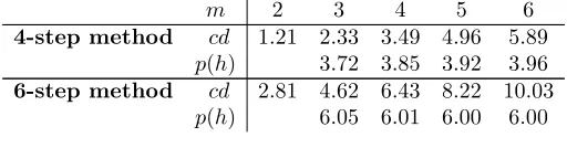
with several integer values ofk.In the following tables, the maximal end point error is written as 10−cd, where cd is the number of correct significant digits. Also, a numerical estimation of the order of convergence of the methods is computed by the formulap(h) = log2(
e(2h)
e(h)),where e(h) is the maximal absolute end point error.
Table 1. The results of problem I.
m 2 3 4 5 6 7
3-step method cd 0.21 1.64 2.74 3.75 4.71 5.63
p(h) 4.76 3.68 3.33 3.17 3.08
4-step method cd 1.02 2.66 4.11 5.43 6.71 5.63
p(h) 5.42 4.79 4.41 4.21 4.11
6-step method cd 2.37 4.19 6.00 7.81 9.62 12.36
p(h) 6.05 6.01 6.00 6.00 6.00
Table 2. The results of problem II.
m 2 3 4 5 6 7
3-step method cd 4.44 5.38 6.31 7.22 8.12 9.03
p(h) 3.12 3.05 3.03 3.02 3.01
4-step method cd 3.91 5.19 6.41 7.64 8.86 10.08
p(h) 4.25 4.06 4.09 4.07 4.04
Table 3. The results of problem III.
m 2 3 4 5 6
4-step method cd 1.21 2.33 3.49 4.96 5.89
p(h) 3.72 3.85 3.92 3.96
6-step method cd 2.81 4.62 6.43 8.22 10.03
p(h) 6.05 6.01 6.00 6.00
References
[1] O.A. Akinfenwa, S.N. Jator and N.M. Yao,Continuous block backward differentiation formula for solving ordinary differential equations, Comput. and math. with appl.65, (2013), 996–1005. [2] C.T.H. Baker, A. Makroglou and E. Short,Regions of stability in the numerical treatment of
Volterra integro-differential equations, SIAM. J. Numer. Anal.16, (1979), 890–910.
[3] J.E. Bond and J.R. Cash,A block method for the numerical integration of stiff sytems of ODEs, BIT,19, (1979), 429–447.
[4] H. Brunner and P. J. Van der Houwen, The Numerical solution of Volterra equations, CWI monographs,3, North Holland, Amesterdam, 1986.
[5] H. Brunner,Collocation methods for Volterra integral and related functional equations, Cam-bridge University Press, 2004.
[6] H. Brunner and J. D. Lambert,Stability of numerical methods for Volterra integro-differential equations, Computing (Arch. Elektron. Rechnen)12, no. 1, (1974), 75–89.
[7] C. W. Gear,Numerical initial value problems in ordinary differential equations,COMM. ACM,
14, (1971), 185–190.
[9] J. D. Lambert,Numerical Methods for Ordinary Differential Systems, Wiley, New York, 1991. [10] T. Lin, Y. Lin, M. Rao and S. Zhang, Petrov-Galerkin methods for linear Volterra
integro-differential equations, SIAM J. Numer. Anal.38, (2000), 937-963.
[11] P. Linz,Linear multistep methods for Volterra integro-differential equations, J. Ass. comput. Mach.16, (1969), 295–301.
[12] J. Matthys,A-stable linear multistep methods for Volterra integro-differential equations, Numer. Math.27, (1976/77), 85–94.
[13] G. Mehdiyeva, M. Imanova and V. Ibrahimov,Application of the Hybrid methods to solving Volterra integro-differential equations,World Academy of Science, Engineering and Technology
77, 2011.
[14] W. E. Milne,Numerical solution of differential equations, John Wiley and Sons, 1953. [15] V. Volterra,Theory of functional and of integral and integro-differential equations, Moscow,
Nauka, 1982.