Notes on nonnegative tensor factorization of the
spectrogram for audio source separation : statistical
insights and towards self-clustering of the spatial cues
C´
edric F´
evotte, Alexey Ozerov
To cite this version:
C´
edric F´
evotte, Alexey Ozerov. Notes on nonnegative tensor factorization of the spectrogram
for audio source separation : statistical insights and towards self-clustering of the spatial cues.
7th International Symposium on Computer Music Modeling and Retrieval (CMMR 2010), Oct
2010, M´
alaga, Spain. pp.www.cmmr2010.etsit.uma.es, 2010.
<
inria-00553355
>
HAL Id: inria-00553355
https://hal.inria.fr/inria-00553355
Submitted on 7 Jan 2011
HAL
is a multi-disciplinary open access
archive for the deposit and dissemination of
sci-entific research documents, whether they are
pub-lished or not.
The documents may come from
teaching and research institutions in France or
abroad, or from public or private research centers.
L’archive ouverte pluridisciplinaire
HAL
, est
destin´
ee au d´
epˆ
ot et `
a la diffusion de documents
scientifiques de niveau recherche, publi´
es ou non,
´
emanant des ´
etablissements d’enseignement et de
recherche fran¸
cais ou ´
etrangers, des laboratoires
publics ou priv´
es.
spectrogram for audio source separation :
statistical insights and towards self-clustering of
the spatial cues
C´edric F´evotte1∗ and Alexey Ozerov21 CNRS LTCI; Telecom ParisTech - Paris, France
2 IRISA; INRIA - Rennes, France
Abstract. Nonnegative tensor factorization (NTF) of multichannel spec-trograms under PARAFAC structure has recently been proposed by Fitzgeraldet al as a mean of performing blind source separation (BSS)
of multichannel audio data. In this paper we investigate the statistical source models implied by this approach. We show that it implicitly as-sumes a nonpoint-source model contrasting with usual BSS assumptions and we clarify the links between the measure of fit chosen for the NTF and the implied statistical distribution of the sources. While the original approach of Fitzgeralet al requires a posterior clustering of the spatial
cues to group the NTF components into sources, we discuss means of performing the clustering within the factorization. In the results section we test the impact of the simplifying nonpoint-source assumption on underdetermined linear instantaneous mixtures of musical sources and discuss the limits of the approach for such mixtures.
Key words: Nonnegative tensor factorization (NTF), audio source sep-aration, nonpoint-source models, multiplicative parameter updates
1
Introduction
Nonnegative matrix factorization (NMF) is an unsupervised data decomposi-tion technique with growing popularity in the fields of machine learning and signal/image processing [1]. Much research about this topic has been driven by applications in audio, where the data matrix is taken as the magnitude or power spectrogram of a sound signal. NMF was for example applied with success to automatic music transcription [2] and audio source separation [3, 4]. The fac-torization amounts to decomposing the spectrogram data into a sum of rank-1
∗This work was supported in part by project ANR-09-JCJC-0073-01 TANGERINE
(Theory and applications of nonnegative matrix factorization) and by the Quaero Programme, funded by OSEO, French State agency for innovation.
spectrograms, each of which being the expression of an elementary spectral pat-tern amplitude-modulated in time.
However, while most music recordings are available in multichannel format (typically, stereo), NMF in its standard setting is only suited to single-channel data. Extensions to multichannel data have been considered, either by stack-ing up the spectrograms of each channel into a sstack-ingle matrix [5] or by equiva-lently considering nonnegative tensor factorization (NTF) under a parallel fac-tor analysis (PARAFAC) structure, where the channel spectrograms form the slices of a 3-valence tensor [6, 7]. Let Xi be the short-time Fourier transform
(STFT) of channel i, a complex-valued matrix of dimensions F ×N, where i = 1, . . . , I and I is the number of channel (I = 2 in the stereo case). The latter approaches boil down to assuming that the magnitude spectrograms|Xi|
are approximated by a linear combination of nonnegative rank-1 “elementary” spectrograms|Ck|=wkhTk such that
|Xi| ≈ K
X
k=1
qik|Ck| (1)
and|Ck|is the matrix containing the modulus of the coefficients of some “latent”
components whose precise meaning we will attempt to clarify in this paper. Equivalently, Eq. (1) writes
|xif n| ≈ K
X
k=1
qikwf khnk (2)
where {xif n} are the coefficients of Xi. Introducing the nonnegative matrices
Q ={qik}, W ={wf k}, H = {hnk}, whose columns are respectively denoted
qk,wk and hk, the following optimization problem needs to be solved
min Q,W,H X if n d(|xif n||vˆif n) subject to Q,W,H≥0 (3) with ˆ vif n def = K X k=1 qikwf khnk (4)
and where the constraintA≥0 means that the coefficients of matrixAare non-negative, andd(x|y) is a scalar cost function, taken as the generalized Kullback-Leibler (KL) divergence in [6] or as the Euclidean distance in [5]. Complex-valued STFT estimates ˆCkare subsequently constructed using the phase of the
observa-tions (typically, ˆckf nis given the phase ofxif n, wherei= argmax{qik}i [7]) and
then inverted to produce time-domain components. The components pertaining to same “sources” (e.g, instruments) can then be grouped either manually or via clustering of the estimated spatial cues{qk}k.
In this paper we build on these previous works and bring the following con-tributions :
– We recast the approach of [6] into a statistical framework, based on a gen-erative statistical model of the multichannel observations X. In particular we discuss NTF of the power spectrogram |X|2 with the Itakura-Saito (IS)
divergence and NTF of the magnitude spectrogram |X| with theKL diver-gence.
– We describe a NTF with a novel structure, that allows to take care of the clustering of the componentswithin the decomposition, as opposed toafter. The paper is organized as follows. Section 2 describes the generative and statistical source models implied by NTF. Section 3 describes new and existing multiplicative algorithms for standard NTF and for “Cluster NTF”. Section 4 reports experimental source separation results on musical data; we test in par-ticular the impact of the simplifying nonpoint-source assumption on underdeter-mined linear instantaneous mixtures of musical sources and point out the limits of the approach for such mixtures. We conclude in Section 5. This article builds on related publications [8, 9].
2
Statistical models to NTF
2.1 Models of multichannel audio
Assume a multichannel audio recording withIchannelsx(t) = [x1(t), . . . , xI(t)]T,
also referred to as “observations” or “data”, generated as a linear mixture of sound source signals. The term “source” refers to the production system, for example a musical instrument, and the term “source signal” refers to the signal produced by that source. When the intended meaning is clear from the context we will simply refer to the source signals as “the sources”.
Under the linear mixing assumption, the multichannel data can be expressed as x(t) = J X j=1 sj(t) (5)
whereJis the number of sources andsj(t) = [s1j(t), . . . sij(t), . . . , sIj(t)]T is the
multichannel contribution of sourcej to the data. Under the common assump-tions of point-sources and linear instantaneous mixing, we have
sij(t) =sj(t)aij (6)
where the coefficients{aij}define aI×Jmixing matrixA, with columns denoted
[a1, . . . ,aJ]. In the following we will show that the NTF techniques described
in this paper correspond to maximum likelihood (ML) estimation of source and mixing parameters in a model where the point-source assumption is dropped and replaced by
sij(t) =s
(i)
where the signals s(ji)(t), i = 1, . . . , I are assumed to share a certain “resem-blance”, as modelled by being two different realizations of the same random process, characterizing their time-frequency behavior, as opposed to be the same realization. Dropping the point-source assumption may also be viewed as ig-noring some mutual information between the channels (assumption of sources contributing to each channel with equal statistics instead of contributing the samesignal). Of course, when the data has been generated from point-sources, dropping this assumption will usually lead to a suboptimal but typically faster separation algorithm, and the results section will illustrate this point.
In this work we further model the source contributions as a sum of elementary components themselves, so that
s(ji)(t) =
X
k∈Kj
c(ki)(t) (8)
where [K1, . . . ,KJ] denotes a nontrivial partition of [1, . . . , K]. As will become
more clear in the following, the components c(ki)(t) will be characterized by a spectral shapewkand a vector of activation coefficientshk, through a statistical
model. Finally, we obtain
xi(t) = K X k=1 mikc( i) k (t) (9)
where mik is defined asmik =aij if and only if k∈ Kj. By linearity of STFT,
model (8) writes equivalently
xif n= K X k=1 mikc( i) kf n (10) where xif n and c( i)
kf n are the complex-valued STFTs of xi(t) and c
(i)
k (t), and
where f = 1, . . . , F is a frequency bin index andn = 1, . . . , N is a time frame index.
2.2 A statistical interpretation of KL-NTF
DenoteVtheI×F×N tensor with coefficientsvif n=|xif n|andQtheI×K
matrix with elements |mik|. Let us assume so far for ease of presentation that
J =K, i.e,mik =aik, so thatMis a matrix with no particular structure. Then
it can be easily shown that the approach of [6], briefly described in Section 1 and consisting in solving
min
Q,W,H
X
if n
with ˆvif ndefined by Eq. (4), is equivalent to ML estimation ofQ,WandHin
the following generative model : |xif n|=
X
k
|mik| |c(kf ni) | (12)
|c(kf ni) | ∼ P(wf khnk) (13)
where P(λ) denotes the Poisson distribution, defined in Appendix A, and the KL divergencedKL(·|·) is defined as
dKL(x|y) =xlog
x
y +y−x. (14)
The link between KL-NMF/KL-NTF and inference in composite models with Poisson components has been established in many previous publications, see, e.g, [10, 11]. In our opinion, model (12)-(13) suffers from two drawbacks. First, the linearity of the mixing model is assumed on the magnitude of the STFT frames -see Eq. (12) - instead of the frames themselves - -see Eq. (10) -, which inherently assumes that the components{c(kf ni) }khave the same phase and that the mixing
parameters{mik}k have the same sign, or that only one component is active in
every time-frequency tile (t, f). Second, the Poisson distribution is formally only defined on integers, which impairs rigorous statistical interpretation of KL-NTF on non-countable data such as audio spectra.
Given estimatesQ,WandHof the loading matrices, Minimum Mean Square Error (MMSE) estimates of the component amplitudes are given by
\
|c(kf ni) |def= E{ |ckf n(i) | |Q,W,H,|X| } (15) = Pqikwf khnk
lqilwf lhnl
|xif n| (16)
Then, time-domain componentsc(ki)(t) are reconstructed through inverse-STFT
ofc(kf ni) =|c\
(i)
kf n|arg(xif n), where arg(x) denotes the phase of complex-valuedx.
2.3 A statistical interpretation of IS-NTF
To remedy the drawbacks of the KL-NTF model for audio we describe a new model based on IS-NTF of the power spectrogram, along the line of [12] and also introduced in [8]. The model reads
xif n= X k mikc( i) kf n (17) c(kf ni) ∼ Nc(0|wf khnk) (18)
where Nc(µ, σ2) denotes the proper complex Gaussian distribution, defined in
estimation ofQ,WandH in model (17)-(18) amounts to solving min Q,W,H X if n dIS(vif n|ˆvif n) subject to Q,W,H≥0 (19)
wheredIS(·|·) denotes the IS divergence defined as
dIS(x|y) =
x y −log
x
y −1. (20)
Note that our notations are abusive in the sense that the mixing parameters |mik| and the components |ckf n| appearing through their modulus in Eq. (12)
are in no way the modulus of the mixing parameters and the components ap-pearing in Eq. (17). Similarly, the matricesWandHrepresent different types of quantities in every case; in Eq. (13) their product is homogeneous to component magnitudes while in Eq. (18) their product is homogeneous to variances of com-ponent variances. Formally we should have introduced variables |cKL
kf n|, W KL,
HKL to be distinguished from variables cISkf n, W
IS, HIS, but we have not in
order to avoid cluttering the notations. The difference between these quantities should be clear from the context.
Model (17)-(18) is a truly generative model in the sense that the linear mix-ing assumption is made on the STFT frames themselves, which is a realistic assumption in audio. Eq. (18) defines a Gaussian variance model of c(kf ni) ; the zero mean assumption reflects the property that the audio frames taken as the input of the STFT can be considered centered, for typical window size of about 20 ms or more. The proper Gaussian assumption means that the phase of c(kf ni) is assumed to be a uniform random variable [13], i.e., the phase is taken into the model, but in a noninformative way. This contrasts from model (12)-(13), which simply discards the phase information.
Given estimatesQ,WandHof the loading matrices, Minimum Mean Square Error (MMSE) estimates of the components are given by
ˆ c(kf ni) def = E{c(kf ni) |Q,W,H,X} (21) = Pqikwf khnk lqilwf lhnl xif n (22)
We would like to underline that the MMSE estimator of components in the STFT domain (21) is equivalent (thanks to the linearity of the STFT and its inverse) to the MMSE estimator of components in the time domain, while the the MMSE estimator of STFT magnitudes (15) for KL-NTF is not consistent with time domain MMSE. Equivalence of an estimator with time domain signal squared error minimization is an attractive property, at least because it is consistent with a popular objective source separation measure such as signal to distortion ratio (SDR) defined in [14].
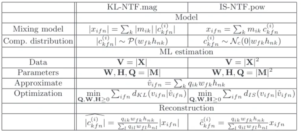
The differences between the two models, termed “KL-NTF.mag” and “IS-NTF.pow” are summarized in Table 1.
KL-NTF.mag IS-NTF.pow Model Mixing model |xif n|= P k|mik| |c( i) kf n| xif n= P kmikc( i) kf n Comp. distribution |c(kf ni) | ∼ P(wf khnk) c( i) kf n∼ Nc(0|wf khnk) ML estimation Data V=|X| V=|X|2 Parameters W,H,Q=|M| W,H,Q=|M|2 Approximate ˆvif n=Pkqikwf khnk Optimization min Q,W,H≥0 P if ndKL(vif n|vˆif n) min Q,W,H≥0 P if ndIS(vif n|vˆif n) Reconstruction \ |c(kf ni) |= qikwf khnk P lqilwf lhnl|xif n| ˆc (i) kf n= qikwf khnk P lqilwf lhnlxif n
Table 1.Statistical models and optimization problems underlaid to KL-NTF.mag and IS-NTF.pow
3
Algorithms for NTF
3.1 Standard NTF
We are now left with an optimization problem of the form min Q,W,HD(V| ˆ V)def= X if n d(vif n|ˆvif n) subject to Q,W,H≥0 (23)
where ˆvif n=Pkqikhnkwf k, andd(x|y) is the cost function, either the KL or IS
divergence in our case. Furthermore we imposekqkk1= 1 andkwkk1= 1, so as
to remove obvious scale indeterminacies between the three loading matricesQ,
W and H. With these conventions, the columns of Qconvey normalized mix-ing proportions (spatial cues) between the channels, the columns ofW convey normalized frequency shapes and all time-dependent amplitude information is relegated intoH.
As common practice in NMF and NTF, we employ multiplicative algorithms for the minimization ofD(V|Vˆ). These algorithms essentially consist of updating each scalar parameter θ by multiplying its value at previous iteration by the ratio of the negative and positive parts of the derivative of the criterion w.r.t. this parameter, namely
θ←θ[∇θD(V|Vˆ)]− [∇θD(V|Vˆ)]+
, (24)
where∇θD(V|Vˆ) = [∇θD(V|Vˆ)]+−[∇θD(V|Vˆ)]−and the summands are both
nonnegative [12]. This scheme automatically ensures the nonnegativity of the pa-rameter updates, provided initialization with a nonnegative value. The derivative of the criterion w.r.t scalar parameterθ writes
∇θD(V|Vˆ) =
X
if n
whered′(x|y) =∇yd(x|y). As such, we get ∇qikD(V|Vˆ) = X f n wf khnkd′(vif n|vˆif n) (26) ∇wf kD(V|Vˆ) = X in qikhnk d′(vif n|vˆif n) (27) ∇hnkD(V|Vˆ) = X if qikwf k d′(vif n|ˆvif n) (28)
We note in the followingGtheI×F×Ntensor with entriesgif n=d′(vif n|vˆif n).
For the KL and IS cost functions we have d′KL(x|y) = 1− x y (29) d′IS(x|y) = 1 y − x y2 (30)
LetAandBbeF×K andN×K matrices. We denoteA◦BtheF×N×K tensor with elementsaf kbnk, i.e, each frontal slicekcontains the outer product
akbTk.
3Now we note<S,T>
KS,KT the contracted product between tensorsS
and T, defined in Appendix B, whereKS and KT are the sets of mode indices
over which the summation takes place. With these definitions we get
∇QD(V|Vˆ) =<G,W◦H>{2,3},{1,2} (31)
∇WD(V|Vˆ) =<G,Q◦H>{1,3},{1,2} (32)
∇HD(V|Vˆ) =<G,Q◦W>{1,2},{1,2} (33)
and multiplicative updates are obtained as
Q←Q.<G−,W◦H>{2,3},{1,2} <G+,W◦H>{2,3},{1,2} (34) W←W.<G−,Q◦H>{1,3},{1,2} <G+,Q◦H>{1,3},{1,2} (35) H←H.<G−,Q◦W>{1,2},{1,2} <G+,Q◦W>{1,2},{1,2} (36) The resulting algorithm can easily be shown to nonincrease the cost function at each iteration by generalizing existing proofs for KL-NMF [15] and for IS-NMF [16]. In our implementation normalization of the variables is carried out at the end of every iteration by dividing every column ofQby theirℓ1norm and scaling
the columns ofWaccordingly, then dividing the columns ofWby theirℓ1norm
and scaling the columns ofH accordingly.
3 This is similar to the Khatri-Rao product of Aand B, which returns a matrix of
3.2 Cluster NTF
For ease of presentation of the statistical composite models inherent to NTF, we have assumed in Section 2.2 and onwards thatK=J, i.e., that one sourcesj(t)
is one elementary componentck(t) with its own mixing parameters {aik}i. We
now turn back to our more general model (9), where each sourcesj(t) is a sum
of elementary components {ck(t)}k∈Kj sharing same mixing parameters{aik}i,
i.e,mik =aij iffk∈ Kj. As such, we can expressMas
M=A L (37)
where Ais the I×J mixing matrix and Lis a J×K “labelling matrix” with only one nonzero value per column, i.e., such that
ljk= 1 iff k∈ Kj (38)
ljk= 0 otherwise. (39)
This specific structure ofM transfers equivalently toQ, so that
Q=DL (40)
where
D=|A| in KL-NTF.mag (41)
D=|A|2 in IS-NTF.pow (42)
The structure of Q defines a new NTF, which we refer to as Cluster NTF, denoted cNTF. The minimization problem (23) is unchanged except for the fact that the minimization over Q is replaced by a minimization over D. As such, the derivatives w.r.t.wf k,hnk do not change and the derivatives overdij write
∇dijD(V|Vˆ) = X f n (X k ljkwf khnk)d′(vif n|ˆvif n) (43) =X k ljk X f n wf khnkd′(vif n|ˆvif n) (44) i.e., ∇DD(V|Vˆ) =<G,W◦H>{2,3},{1,2}LT (45)
so that multiplicative updates forDcan be obtained as
D←D.<G−,W◦H>{2,3},{1,2}L
T
<G+,W◦H>{2,3},{1,2}LT
(46) As before, we normalize the columns ofDby theirℓ1 norm at the end of every
iteration, and scale the columns ofWaccordingly.
In our Matlab implementation the resulting multiplicative algorithm for IS-cNTF.pow is 4 times faster than the one presented in [8] (for linear in-stantaneous mixtures), which was based on sequential updates of the matri-ces [qk]k∈Kj, [wk]k∈Kj, [hk]k∈Kj. The Matlab code of this new algorithm as
well as the other algorithms described in this paper can be found online at http://perso.telecom-paristech.fr/~fevotte/Samples/CMMR10/.
4
Results
We consider source separation of simple audio mixtures taken from the Signal Separation Evaluation Campaign (SiSEC 2008) website. More specifically, we used some “development data” from the “underdetermined speech and music mixtures task” [17]. We considered the following datasets :
– wdrums, a linear instantaneous stereo mixture (with positive mixing coeffi-cients) of 2 drum sources and 1 bass line,
– nodrums, a linear instantaneous stereo mixture (with positive mixing co-efficients) of 1 rhythmic acoustic guitar, 1 electric lead guitar and 1 bass line.
The signals are of length 10 sec and sampled at 16 kHz. We applied a STFT with sine bell of length 64 ms (1024 samples) leading toF = 513 andN = 314. We applied the following algorithms to the two datasets :
– KL-NTF.mag withK= 9,
– IS-NTF.pow withK= 9,
– KL-cNTF.mag withJ= 3 and 3 components per source, leading toK= 9,
– IS-cNTF.pow withJ = 3 and 3 components per source, leading toK= 9. Every four algorithm was run 10 times from 10 random initializations for 1000 it-erations. For every algorithm we then selected the solutionsQ,WandHyielding smallest cost value. Time-domain components were reconstructed as discussed in Section 2.2 for KL-NTF.mag and KL-cNTF.mag and as is in Section 2.3 for IS-NTF.pow and IS-cNTF.pow. Given these reconstructed components, source estimates were formed as follows :
– For KL-cNTF.mag and IS-cNTF.pow, sources are immediately computed using Eq. (8), because the partitionK1, . . . ,KJ is known.
– For KL-NTF.mag and IS-NTF.pow, we used the approach of [6, 7] consisting of applying the K-means algorithm toQ(withJclusters) so as to label every componentk to a sourcej, and each of the J sources is then reconstructed as the sum of its assigned components.
Note that we are here not reconstructing the original single-channel sources sj(t) but their multichannel contribution [s(1)j (t), . . . , s
(I)
j (t)] to the
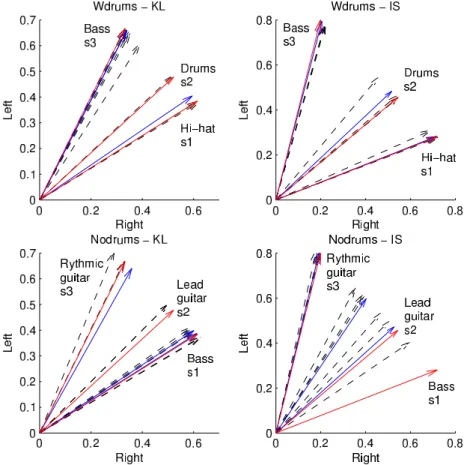
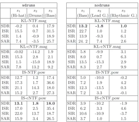
multichan-nel data (i.e, their spatial image). The quality of the source image estimates was assessed using the standard Signal to Distortion Ratio (SDR), source Im-age to Spatial distortion Ratio (ISR), Source to Interference Ratio (SIR) and Source to Artifacts Ratio (SAR) defined in [18]. The numerical results are reported in Table 2. The source estimates may also be listened to online at http://perso.telecom-paristech.fr/~fevotte/Samples/CMMR10/. Figure 1 displays estimated spatial cues together with ground truth mixing matrix, for every method and dataset.
Discussion On dataset wdrums best results are obtained with IS-cNTF.pow. Top right plot of Figure 1 shows that the spatial cues returned byDreasonably fit the original mixing matrix|A|2. The slightly better results of IS-cNTF.pow
compared to IS-NTF.pow illustrates the benefit of performing clustering of the spatial cues within the decomposition as opposed to after. On this dataset KL-cNTF.mag fails to adequately estimate the mixing matrix. Top left plot of Fig-ure 1 shows that the spatial cues corresponding to the bass and hi-hat are cor-rectly captured, but it appears that two columns ofDare “spent” on representing the same direction (bass, s3), suggesting that more components are needed to
represent the bass, and failing to capture the drums, which are poorly estimated. KL-NTF.mag performs better (and as such, one spatial cueqk is correctly fitted
to the drums direction) but overly not as well as IS-NTF.pow and IS-cNTF.pow. On dataset nodrums best results are obtained with KL-NTF.mag. None of the other methods adequately fits the ground truth spatial cues. KL-cNTF.mag suffers same problem than on datasetwdrums : two columns ofD are spent on the bass. In contrast, none of the spatial cues estimated by IS-NTF.pow and IS-cNTF.pow accurately captures the bass direction, and ˆs1and ˆs2both contain
much bass and lead guitar.4 Results from all four methods on this dataset are
overly all much worse than with dataset wdrums, corroborating an established idea than percussive signals are favorably modeled by NMF models [19]. In-creasing the number of total componentsK did not seem to solve the observed deficiencies of the 4 approaches on this dataset.
5
Conclusions
In this paper we have attempted to clarify the statistical models latent to audio source separation using PARAFAC-NTF of the magnitude or power spectro-gram. In particular we have emphasized that the PARAFAC-NTF does not op-timally exploits interchannel redundancy in the presence of point-sources. This still may be sufficient to estimate spatial cues correctly in linear instantaneous mixtures, in particular when the NMF model suits well the sources, as seen from the results on datasetwdrumsbut may also lead to incorrect results in other cases, as seen from results on dataset nodrums. In contrast methods fully exploiting interchannel dependencies, such as the EM algorithm based on model (17)-(18) with c(kf ni) =ckf n in [8], can successfully estimates the mixing matrix in both
datasets. The latter method is however about 10 times computationally more demanding than IS-cNTF.pow.
In this paper we have considered a variant of PARAFAC-NTF in which the loading matrixQis given a structure such thatQ=DL. We have assumed that
4 The numerical evaluation criteria were computed using the bss eval.m function
available from SiSEC website. The function automatically pairs source estimates with ground truth signals according to best mean SIR. This resulted here in pairing left, middle and right blue directions with respectively left, middle and right red directions, i.e, preserving the panning order.
Fig. 1.Mixing parameters estimation and ground truth. Top : wdrums dataset. Bot-tom : nodrums dataset. Left : results of KL-NTF.mag and KL-cNTF.mag; ground truth mixing vectors{|aj|}j(red), mixing vectors{dj}jestimated with KL-cNTF.mag
(blue), spatial cues{qk}kgiven by KL-NTF.mag (dashed, black). Right : results of
IS-NTF.pow and IS-cIS-NTF.pow; ground truth mixing vectors{|aj|2}j(red), mixing vectors
{dj}j estimated with IS-cNTF.pow (blue), spatial cues{qk}k given by IS-NTF.pow
wdrums
s1 s2 s3
(Hi-hat) (Drums) (Bass) KL-NTF.mag SDR -0.2 0.4 17.9 ISR 15.5 0.7 31.5 SIR 1.4 -0.9 18.9 SAR 7.4 -3.5 25.7 KL-cNTF.mag SDR -0.02 -14.2 1.9 ISR 15.3 2.8 2.1 SIR 1.5 -15.0 18.9 SAR 7.8 13.2 9.2 IS-NTF.pow SDR 12.7 1.2 17.4 ISR 17.3 1.7 36.6 SIR 21.1 14.3 18.0 SAR 15.2 2.7 27.3 IS-cNTF.pow SDR 13.1 1.8 18.0 ISR 17.0 2.5 35.4 SIR 22.0 13.7 18.7 SAR 15.9 3.4 26.5 nodrums s1 s2 s3
(Bass) (Lead G.) (Rhythmic G.) KL-NTF.mag SDR 13.2 -1.8 1.0 ISR 22.7 1.0 1.2 SIR 13.9 -9.3 6.1 SAR 24. 2 7.4 2.6 KL-cNTF.mag SDR 5.8 -9.9 3.1 ISR 8.0 0.7 6.3 SIR 13.5 -15.3 2.9 SAR 8.3 2.7 9.9 IS-NTF.pow SDR 5.0 -10.0 -0.2 ISR 7.2 1.9 4.2 SIR 12.3 -13.5 0.3 SAR 7.2 3.3 -0.1 IS-cNTF.pow SDR 3.9 -10.2 -1.9 ISR 6.2 3.3 4.6 SIR 10.6 -10.9 -3.7 SAR 3.7 1.0 1.5
Table 2.SDR, ISR, SIR and SAR of source estimates for the two considered datasets. Higher values indicate better results. Values in bold font indicate the results with best average SDR.
Lis known labelling matrix that reflects the partitionK1, . . . ,KJ. An important
perspective of this work is to let the labelling matrix free and automatically estimate it from the data, either under the constraint that every columnlk ofL
may contain only one nonzero entry, akin to a hard clustering, i.e.,klkk0= 1, or
more generally under the constraint thatklkk0 is small, akin to soft clustering.
This should be made feasible using NTF under sparseℓ1-constraints and is left
for future work.
A
Standard distributions
Proper complex Gaussian Nc(x|µ,Σ) =|πΣ|−1exp−(x−µ)HΣ−1(x−µ)
Poisson P(x|λ) = exp(−λ)λxx!
B
Contracted tensor product
LetSbe a tensor of sizeI1×. . .×IM×J1×. . .×JN andTbe a tensor of sizeI1×
. . .×IM×K1×. . .×KP. Then, the contracted product<S,T>{1,...,M},{1,...,M}
is a tensor of sizeJ1×. . .×JN ×K1×. . .×KP, given by
<S,T>{1,...,M},{1,...,M}= I1 X i1=1 . . . IM X iM=1 si1,...,iM,j1,...,jNti1,...,iM,k1,...,kP (47)
The contracted tensor product should be thought of as a form a generalized dot product of two tensors along common modes of same dimensions.
References
1. Lee, D.D., Seung, H.S.: Learning the parts of objects with nonnegative matrix factorization. Nature401(1999) 788–791
2. Smaragdis, P., Brown, J.C.: Non-negative matrix factorization for polyphonic mu-sic transcription. In: IEEE Workshop on Applications of Signal Processing to Audio and Acoustics (WASPAA’03). (Oct. 2003)
3. Virtanen, T.: Monaural sound source separation by non-negative matrix factor-ization with temporal continuity and sparseness criteria. IEEE Transactions on Audio, Speech and Language Processing15(3) (Mar. 2007) 1066–1074
4. Smaragdis, P.: Convolutive speech bases and their application to speech separation. IEEE Transactions on Audio, Speech, and Language Processing15(1) (Jan. 2007) 1–12
5. Parry, R.M., Essa, I.A.: Estimating the spatial position of spectral components in audio. In: Proc. 6th International Conference on Independent Component Analysis and Blind Signal Separation (ICA’06), Charleston SC, USA (Mar. 2006) 666–673 6. FitzGerald, D., Cranitch, M., Coyle, E.: Non-negative tensor factorisation for
sound source separation. In: Proc. of the Irish Signals and Systems Conference, Dublin, Ireland (Sep. 2005)
7. FitzGerald, D., Cranitch, M., Coyle, E.: Extended nonnegative tensor factorisa-tion models for musical sound source separafactorisa-tion. Computafactorisa-tional Intelligence and Neuroscience2008(Article ID 872425) (2008) 15 pages
8. Ozerov, A., F´evotte, C.: Multichannel nonnegative matrix factorization in convo-lutive mixtures for audio source separation. IEEE Transactions on Audio, Speech and Language Processing18(3) (2010) 550–563
9. F´evotte, C.: Itakura-Saito nonnegative factorizations of the power spectrogram for music signal decomposition. In Wang, W., ed.: Machine Audition: Principles, Algorithms and Systems. IGI Publishing (to appear)
10. Cemgil, A.T.: Bayesian inference for nonnegative matrix factorisation models. Computational Intelligence and Neuroscience2009(Article ID 785152) (2009) 17 pages doi:10.1155/2009/785152.
11. Shashua, A., Hazan, T.: Non-negative tensor factorization with applications to statistics and computer vision. In: Proc. 22nd International Conference on Machine learning, Bonn, Germany, ACM (2005) 792 – 799
12. F´evotte, C., Bertin, N., Durrieu, J.L.: Nonnegative matrix factorization with the Itakura-Saito divergence. With application to music analysis. Neural Computation
21(3) (Mar. 2009) 793–830
13. Neeser, F.D., Massey, J.L.: Proper complex random processes with applications to information theory. IEEE Transactions on Information Theory39(4) (Jul. 1993) 1293–1302
14. Vincent, E., Gribonval, R., F´evotte, C.: Performance measurement in blind audio source separation. IEEE Transactions on Audio, Speech and Language Processing
14(4) (Jul. 2006) 1462–1469
15. Shepp, L.A., Vardi, Y.: Maximum likelihood reconstruction for emission tomogra-phy. IEEE Transactions on Medical Imaging1(2) (Oct. 1982) 113–122
16. Cao, Y., Eggermont, P.P.B., Terebey, S.: Cross Burg entropy maximization and its application to ringing suppression in image reconstruction. IEEE Transactions on Image Processing8(2) (Feb. 1999) 286–292
17. Vincent, E., Araki, S., Bofill, P.: Signal Separation Evaluation Campaign (SiSEC 2008) / Under-determined speech and music mixtures task results (2008) http: //www.irisa.fr/metiss/SiSEC08/SiSEC_underdetermined/dev2_eval.html. 18. Vincent, E., Sawada, H., Bofill, P., Makino, S., Rosca, J.P.: First stereo audio
source separation evaluation campaign: Data, algorithms and results. In: Proc. Int. Conf. on Independent Component Analysis and Blind Source Separation (ICA’07), Springer (2007) 552–559
19. Hel´en, M., Virtanen, T.: Separation of drums from polyphonic music using non-negative matrix factorization and support vector machine. In: Proc. 13th European Signal Processing Conference (EUSIPCO’05). (2005)