new test for the parametric form of the variance function in nonparametric regression

econ

stor

www.econstor.eu

Nutzungsbedingungen:

Die ZBW räumt Ihnen als Nutzerin/Nutzer das unentgeltliche, räumlich unbeschränkte und zeitlich auf die Dauer des Schutzrechts beschränkte einfache Recht ein, das ausgewählte Werk im Rahmen der unter

→ http://www.econstor.eu/dspace/Nutzungsbedingungen nachzulesenden vollständigen Nutzungsbedingungen zu vervielfältigen, mit denen die Nutzerin/der Nutzer sich durch die erste Nutzung einverstanden erklärt.

Terms of use:

The ZBW grants you, the user, the non-exclusive right to use the selected work free of charge, territorially unrestricted and within the time limit of the term of the property rights according to the terms specified at

→ http://www.econstor.eu/dspace/Nutzungsbedingungen By the first use of the selected work the user agrees and declares to comply with these terms of use.

zbw

Dette, Holger; van Keilegom, Ingrid

Working Paper

new test for the parametric form of the

variance function in nonparametric

regression

Technical Report / Universität Dortmund, SFB 475 Komplexitätsreduktion in Multivariaten Datenstrukturen, No. 2005,32

Provided in cooperation with:

Technische Universität Dortmund

Suggested citation: Dette, Holger; van Keilegom, Ingrid (2005) : new test for the parametric form of the variance function in nonparametric regression, Technical Report / Universität

Dortmund, SFB 475 Komplexitätsreduktion in Multivariaten Datenstrukturen, No. 2005,32, http:// hdl.handle.net/10419/22622

A new test for the parametric form of the variance function

in nonparametric regression

Holger Dette

Ruhr-Universit¨at Bochum

Ingrid Van Keilegom

Universit´e catholique de Louvain

September 9, 2005

Abstract

In the common nonparametric regression model the problem of testing for the parametric form of the conditional variance is considered. A stochastic process based on the difference between the empirical processes obtained from the standardized nonparametric residuals under the null hypothesis (of a specific parametric form of the variance function) and the alternative is introduced and its weak convergence established. This result is used for the construction of a Cram´er von Mises type statistic for testing the parametric form of the conditional variance. The finite sample properties of a bootstrap version of this test are investigated by means of a simulation study. In particular the new procedure is compared with some of the currently available methods for this problem and its performance is illustrated by means of a data example.

Key Words:

1 _{Financial support of the Deutsche Forschungsgemeinschaft (SFB 475, Komplexit¨atsreduktion} in multivariaten Datenstrukturen, Teilprojekt B1) is gratefully acknowledged. 2 Financial sup-port from the IAP research network nr. P5/24 of the Belgian government (Belgian Science Policy) is gratefully acknowledged.

1

Introduction

Consider the common nonparametric heteroscedastic regression model

Y =m(X) +σ(X)ε, (1.1)

where (X, Y) denotes a random vector, Y is a possible transformation of the variable of interest, X is a covariate, and the centered error variable ε is independent of X with mean 0 and variance 1. The functionm(X) =E(Y_|X) is the unknown regression function andσ2_{(X) = Var(Y|X) is the unknown conditional variance function. The importance of}

being able to test data corresponding to model (1.1) for heteroscedasticity is widely recog-nized because under the additional assumption of homoscedasticity the statistical analysis can be simplified substantially in most cases. On the other hand, if the assumption of homoscedasticity is not met, efficient inference for the regression function requires that the heteroscedasticity is taken into account. This may result in transformations of the data, weighted least squares (or modified likelihood) procedures or the choice of a variable bandwidth in nonparametric kernel smoothing [see M¨uller and Stadtm¨uller (1987)]. Early work on detecting heteroscedasticity is based on diagnostic plots based on resid-uals after fitting a specific regression model to the data. Harrison and McCabe (1979), Breusch and Pagan (1979), Koenker and Bassett (1981), Cook and Weisberg (1983), Car-roll and Ruppert (1988), Sec. 3.4, and Diblasi and Bowman (1997) developed formal tests for the form of the variance function under the additional assumption that a parametric model for the regression function can be specified. A diagnostic test under a smoothness assumption on the regression function and the assumption of a normally distributed er-ror distribution has been proposed by Eubank and Thomas (1993). More recent work on testing homoscedasticity considers a completely nonparametric specification of the regres-sion model (1.1). Dette and Munk (1998) used an estimate of the L2_{-distance between}

the variance function and its integral as test statistic, while Zhu, Fujikoshi and Naito (2001) proposed a test based on a marked empirical process of the squared residuals for testing homoscedasticity. Recently Dette (2002), Liero (2003) and Francisco-Fern´andez and Vilar-Fern´andez (2005) used estimates for the L2_{-distance between the variance}

es-timators in both models – the underlying heteroscedastic model and the hypothetical homoscedastic model – as test statistic.

It is the purpose of the present paper to present an alternative approach for the problem of testing for a parametric form of the variance function in the nonparametric regression model (1.1). Our investigations are mainly motivated by the observation that all papers

on testing homoscedasticity in a completely nonparametric regression model consider test statistics based on squared residuals from a nonparametric fit. In contrast to this approach we are interested in procedures, which use the residuals directly. Our interest in such methods is motivated twofold. On one hand we expect tests based on nonparametric residuals to be more sensitive for detecting deviations from homoscedasticity in the data. On the other hand the consideration of the residuals instead of their squares is more naturally related to the commonly used graphical procedures based on visual examination of the residuals [see Atkinson (1985)].

Moreover, the literature published so far is restricted to tests for homoscedasticity but there are numerous applications where a test for given parametric form of the variance function is required. Thus a further difference to the work cited in the previous paragraph is that we consider the more general problem of testing for a specific parametric form of the variance function (see our formulation of the null hypothesis in Section 2). Finally, in the case of testing for homoscedaticity the test statistic we will develop has the nice property that it can detect local alternatives converging to the null hypothesis of constant variance with a rate faster than root-n, whereas all other existing tests only attain the rate root-nor even slower. We propose to compare the empirical processes of the standardized residuals from a nonparametric fit under the null hypothesis (of a specific parametric form, e.g. homoscedasticity) and under the alternative (e.g. heteroscedasticity) and reject the null hypothesis for large differences between these processes. In Section 2 we present some preliminary notation and a motivation of our approach. Section 3 contains the main results. We derive a stochastic expansion for the difference between the empirical processes of the standardized residuals under the null hypothesis and under the alternative and use this result to prove the weak convergence of the corresponding difference process. As a consequence a Kolmogorov-Smirnov and a Cram´er-von Mises test based on the difference process are proposed. In Section 4 we study the finite sample properties of a bootstrap version of the new test and demonstrate that this procedure yields tests with a reliable approximation of the nominal level and reasonable power. We also compare the test with the currently available methods proposed in Dette and Munk (1998), Zhu, Fujikoshi and Naito (2001), Dette (2002) and Francisco-Fern´andez and Vilar-Fern´andez (2005), and demonstrate that in many cases the new procedure yields substantially larger power in the problem of testing for homoscedasticity. Finally, we analyze data on the concentration of sulfate in rain at two towns in North Carolina. Some technical details are deferred to the Appendix.

2

Notation and motivation of the test statistic

Consider the random vector (X, Y) satisfying model (1.1) and define Fε(y) = P(ε ≤y),

F(y_|x) = P(Y _≤ y_|X = x) and FX(x) = P(X ≤ x) as the distribution function of the

error, the conditional distribution function ofY givenX =xand the distribution function of the predictor, respectively. The probability density functions of Fε(y) and FX(x) are

assumed to exist and will be denoted by fε(y) and fX(x), respectively. We are interested

in a test for the hypothesis

H0 :σ2 ∈ Mversus H1 :σ2 ∈ M/ , (2.1)

where

M={σ_θ2 :θ ∈Θ} (2.2)

is some parametric class of variance functions and Θ ⊂ IRp is a set of parameters satis-fying some regularity conditions, which will be specified in the Appendix. Note that the hypothesis of homoscedasticity is obtained for p= 1, σ2

θ(x) =θ, but (2.1) contains many

other hypotheses of practical interest.

The easiest way to motivate our approach is to consider the problem of testing for the parametric form of the variance function in the nonparametric regression model (1.1) in terms of distribution functions. For this we introduce the random variables

ε = Y −m(X) σ(X) (2.3) and ε0 = Y ₋m(X) σ_θ˜₀(X) , (2.4)

where ˜θ0 ∈ Θ denotes the parameter corresponding to the best approximation of the

variance function σ2 _{by elements of the class M, that is}

˜ θ0 = argmin θ∈Θ E[{(Y −m(X)) 2_−σ2 θ(X)}2] (2.5) = argmin θ∈Θ E[_{σ2(X)₋σ2_θ(X)_}2]. (2.6)

Note that under H0, ˜θ0 equals θ0, the true value of θ. Throughout this paper we assume

that ˜θ0 exists and is uniquely determined. If the null hypothesis

is satisfied, the random variablesε and ε0 defined in (2.3) and (2.4) have the same

distri-bution. In general these distributions are different and we obtain

P(ε0≤y) = P ε_≤ σθ˜0(X) σ(X) y . (2.7)

The following result shows that the equality of the distributions of the random variablesε0

andεis equivalent to the hypothesis (2.1) of a specific parametric form for the conditional variance. The proof can be found in the Appendix.

Lemma 2.1 Assume that all moments of the distribution of the error ε exist. The dis-tributions of the random variables ε andε0 defined in (2.3) and (2.4) coincide if and only

if the hypothesis H0 :σ2 ∈ M={σ2θ | θ∈Θ} is satisfied.

The construction of a test statistic for the hypothesis (2.1) follows exactly the same pattern, where we replace the unknown distributions of the random variablesε and ε0 by

appropriate estimates. For this let (Xi, Yi),i= 1, . . . , n, denote independent replications

of (X, Y). We first estimate the distribution of the errorεin a nonparametric way. Define for any x in the support [a, b] of the distributionFX of X the estimates

ˆ m(x) = n X i=1 Wi(x, h)Yi, σˆ2(x) = n X i=1 Wi(x, h)(Yi−mˆ(Xi))2, (2.8) where Wi(x, h) = Kx−Xi h Pn j=1K _x−X j h (2.9)

are the Nadaraya-Watson weights [see Nadaraya (1964) or Watson (1964)], K is a known probability density function (kernel) and h is an appropriate bandwidth. This leads to

ˆ Fε(y) =n−1 n X i=1 I(ˆεi ≤y), (2.10)

as an estimate of the distribution function Fε, where

ˆ

εi =

Yi−mˆ(Xi)

ˆ

σ(Xi)

are the nonparametric residuals. This estimator (modulo a slightly different variance estimator) has been recently proposed and studied by Akritas and Van Keilegom (2001). Next, under the null hypothesis H0 we estimate the variance function σ2(x) by σ_θ2ˆ(x),

where ˆθ is a minimizer (over θ∈Θ) of the expression

Sn(θ) =n−1 n X i=1

and we smooth the parametric estimate by the same bandwidth and kernel as for the nonparametric estimator ˆσ2_{(x), i.e.}

ˆ σ2₀(x) = n X i=1 Wi(x, h)σ2_θˆ(Xi). This leads to ˆ Fε0(y) =n−1 n X i=1 I(ˆεi0≤ y), (2.12)

as an estimator of the distribution function of the random variable ε0 defined in (2.4),

where ˆ εi0 = Yi−mˆ(Xi) ˆ σ0(Xi)

are the standardized residuals estimated under the null hypothesis H0.

Under the null hypothesis (2.1) one expects not too large deviations between the empirical distribution functions ˆFε0and ˆFε. Consequently we propose the Kolmogorov-Smirnov type

statistic

TKS =n1/2 sup

−∞<y<∞| ˆ

Fε(y)−Fˆε0(y)|

and the Cram´er-von Mises type statistic

TCM =n Z

[ ˆFε(y)−Fˆε0(y)]2dFˆε(y)

for testing the hypothesis (2.1) of a specific parametric form of the variance function in model (1.1).

3

Main results

In the following we will study some asymptotic properties of the these statistics under the null hypothesis (2.1) and under local (Pitman) alternatives of the form

H1 :σ2(·)≡σθ20(·) +n

−1/2_r(

·), (3.1)

for some function r (note that the null hypothesis H0 is obtained for n → ∞). We

introduce the following additional notation: Ω = ( E " ∂σ2 θ(X) ∂θr _θ=θ 0 ∂σ2 θ(X) ∂θs _θ=θ 0 #) r,s=1,...,p , (3.2)

and ∂σ2 θ(x) ∂θ = ∂σ2 θ(x) ∂θr ! r=1,...,p

is the gradient of the variance function σ2

θ with respect to θ = (θ1, . . . , θp)0 (here and

throughout this paper we assume its existence). The assumptions mentioned in the results below can be found in the Appendix, as well as the proofs of Theorems 3.1 and 3.4.

Theorem 3.1 Assume that the conditions (A1)-(A3) in the Appendix are satisfied. Then, under the null hypothesis H0, the following stochastic expansion is valid:

ˆ Fε(y)−Fˆε0(y) = yfε(y) 2 ( n−1 n X i=1 σ−2(Xi)[{Yi−m(Xi)}2−σ2(Xi)] −Z σ−2(x) ∂σ 2 θ(x) ∂θ _θ=θ 0 !0 dFX(x) Ω−1n−1 n X i=1 [{Yi−m(Xi)}2−σ2(Xi)] ∂σ2 θ(Xi) ∂θ _θ=θ 0 ) +Rn(y),

where the random process _{Rn(y)}_y∈IR satisfies

sup

−∞<y<∞|Rn(y)|=oP(n −1/2_).

The first term on the right hand side of the above expansion is the result of estimating the variance function σ2_{(·) nonparametrically by ˆσ}2_{(·), whereas the second term comes from}

the parametric estimator ˆσ2

0(·). Note that the estimation of m(·) does not contribute to

the main term of this expansion. This is because the same estimator of m(·) is used in the expressions of ˆεi and ˆεi0 (i = 1, . . . , n), and hence the contribution of this estimator

to the main term cancels out [see our proof in the Appendix]. The following Corollary is an immediate consequence of Theorem 3.1, since the main term in the above representa-tion factorizes in a deterministic funcrepresenta-tion only dependent on y and a sum of i.i.d. terms independent of y.

Corollary 3.2 Assume that the conditions (A1)-(A3) in the Appendix are satisfied. Then, under the null hypothesis H0, the process {n1/2( ˆFε(y)−Fˆε0(y))}_y∈IR converges weakly to

the process _{yfε(y)W}_y∈IR, where W is a zero-mean normal random variable with

vari-ance Var(W) = 1 4E h ε4 ₋₁i_E   1₋ Z _σ2 θ0(X) σ2 θ0(x) _∂σ2 θ(x) ∂θ θ=θ0 0 dFX(x)Ω−1 ∂σ2 θ(X) ∂θ θ=θ0 !2 .

We are now ready to establish the weak convergence of the test statistics TKS and TCM.

Corollary 3.3 Assume that the conditions (A1)-(A3) in the Appendix are satisfied. Then, under the null hypothesis H0,

TKS →d sup

−∞<y<∞|yfε(y)| |W| ,

TCM →d Z

y2f_ε2(y)dFε(y)W2,

where the random variable W has been defined in Corollary 3.2.

The proof for the statistic TKS follows from the continuous mapping theorem, while for

TCM the proof mimics almost exactly that of Corollary 3.3 in Van Keilegom,

Gonz´alez-Manteiga and S´anchez-Sellero (2005).

Note that the limiting process in Corollary 3.2 has an extremely simple structure, as it factorizes in a deterministic function and a random variable independent of y. However, the deterministic factor depends on the unknown density of the error distribution, which may be difficult to estimate in many cases, although estimators for this density have been proposed and studied in the literature (see e.g. Van Keilegom and Veraverbeke (2002)). Therefore we propose the application of a smoothed bootstrap procedure for the calculation of the critical values (see our discussion in Section 4). We conclude this section considering the limiting behavior of the two test statistics under the local alternative H1

and two illustrative examples.

Theorem 3.4 Assume that the conditions (A1)-(A4) in the Appendix are satisfied. Then, under local alternatives of the form (3.1),

TKS →d sup −∞<y<∞|yfε(y)| |W +b| TCM →d Z y2f_ε2(y)dFε(y) (W +b)2, where b = − Z σ−_θ02(x)∂σ 2 θ(x) ∂θ _θ=θ 0 ₀ dFX(x) Ω−1 Z r(x)∂σ 2 θ(x) ∂θ _θ=θ 0dFX(x) + Z σ_θ−₀2(x)r(x)dFX(x).

Example 3.1 In the important problem of testing for homoscedasticity (i.e.H0 :σ2(·)≡

θ for some θ > 0), it follows that ∂σ2

that the main term of the asymptotic representation in Theorem 3.1 vanishes, i.e. sup

−∞<y<∞| ˆ

Fε(y)−Fˆε0(y)|=oP(n−1/2).

As a consequence the limit distribution in Corollary 3.2, 3.3 and 3.4 degenerates to a Dirac measure concentrated at the point 0. Hence, in the problem of testing for homoscedastic-ity, tests based on the process

{n1/2( ˆFε(y)−Fˆε0(y))}_y∈IR

can detect local alternatives converging to the null hypothesis with a rate faster than root-n.

Example 3.2 The following example shows that one cannot expect that the statement of Example 3.1 is correct for more general hypotheses on the conditional variance. Consider for example the case p= 1 and σ2

θ(x) =θk(x) for a given nonnegative function k. In this

case the distribution of the random variable W is a centered normal with variance Var(W) = 1

4E[ε

4

−1]Var[k2(X)]/E[k2(X)]2,

which vanishes if and only the function k is constant.

4

Finite sample properties and a data example

4.1

A simulation study

In this section we study the finite sample properties of the new test and compare it with four other procedures, which are currently available in the literature for testing for homoscedasticity. We limit attention to the Cram´er-von Mises test and demonstrate that in many cases the new procedure yields a larger power. Note that the asymptotic distribution of this test depends on the unknown density of the error ε. Although this can be estimated in principle, we decided to implement a smooth bootstrap version of the test. To be precise, first define

ε∗_i = ˜εi+vNi i= 1, . . . , n (4.1)

where ˜ε1, . . . ,ε˜nare a sample of i.i.d. observations with distribution function ˆFε,N1, . . . , Nn

is a smoothing parameter. In a next step we generate bootstrap data according to the model

Y_i∗ = ˆm(Xi) +σ_θˆ(Xi)ε∗i,

where σ2 ˆ

θ(·) is the estimate of the variance function under the null hypothesis (2.1), and

calculate the corresponding Cram´er-von Mises statistic T∗

CM from the bootstrap data. If

B bootstrap replications have been performed and T_CM∗(1) < . . . < T_CM∗(B) denote the order statistics of the calculated bootstrap sample, the null hypothesis (2.1) is rejected if

TCM > TCM∗(bB(1−α)c). (4.2)

B = 100 bootstrap replications are performed to calculate the rejection probabilities of the test (4.2) and 1000 simulation runs are used for each scenario. In order to investigate the impact of the bandwidth for the Nadaraya-Watson weights in the testing procedure we considered the two cases h = 0.3 and h = 0.5 and for the factor v in (4.1) we used

v = 0.2.

Example 4.1. Our first example considers the problem of testing for homoscedasticity in the nonparametric regression model (1.1). In particular we consider the nonparametric regression models

(I) m(x) = 1 + sinx σ(x) = σexp(cx)

(II) m(x) = 1 +x σ(x) = σ(1 +c·sin(10x))2

(III) m(x) = 1 +x σ(x) = σ(1 +cx)2_,

(4.3)

where the standard deviation is chosen as σ = 0.5 and the parameter c is given by 0,0.5 and 1.0.In Table 4.1 and 4.2 we show the simulated rejection probabilities for the sample sizes n = 50, 100, 200 and for the two bandwidths h = 0.3 and h = 0.5, respectively. Note that the casec= 0 corresponds to the null hypothesis of homoscedasticity and that the test beds defined by (4.3) were also considered in a simulation study by Dette and Munk (1998), who used an estimate of Var[σ2_{(X)] as test for homoscedasticity. Thus}

our results are directly comparable with the corresponding rejection probabilities given in Table 1 of this reference. The models (I) and (III) have also been considered in Dette (2002), who proposed to estimate Var[σ2_{(X)] by smoothing methods, see Table 1 and}

2 in this reference. Francisco-Fern´andez and Vilar-Fern´andez (2005) investigated Liero’s (2003) proposal to use an L2_{-distance between a nonparametric and a constant estimate}

reference]. These authors propose a further test for homoscedasticity, which is based on a combination of a polynomial least squares fit to the squared nonparametric residuals with a test if this polynomial is constant. Because this test is not consistent in general, it is not included in our comparison.

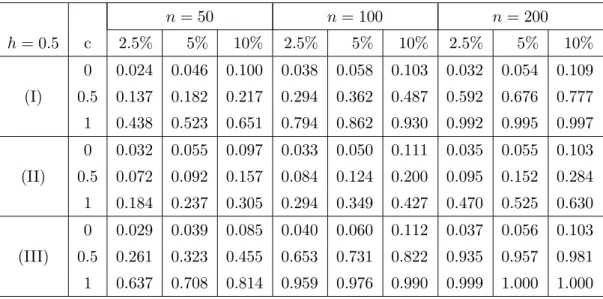
We observe a rather precise approximation of the nominal level by the new test in all cases (see the rows labeled with c = 0 in Table 4.1 and 4.2). Moreover, for model (I) and (III) the impact of the choice of the bandwidth h seems to be less critical compared to the oscillating case (II). In this situation the power of the bootstrap test decreases substantially with an increasing bandwidth. A comparison with the results of Dette and Munk (1998) and Dette (2002) shows that in the test beds (I) and (III) the new test yields substantially larger power than the test proposed by these authors. For example in model (I) with c= 1 the power of the new test at level α= 10% withn= 50 observations is 0.614 and 0.651 corresponding to the cases h = 0.3 and h = 0.5, respectively. This power is even not reached by the test of Dette and Munk (1998) forn = 200 observations, where the power is 0.458. On the other hand the power of Dette’s (2002) test is 0.566 for

n = 50 observations. For a comparison with the test of Francisco-Fern´andez and Vilar-Fern´andez (2005) we have to consider the sample size n= 100, because these authors did not present results for smaller sample sizes. In this case the power of the new procedure is 0.922 (h = 0.3) and 0.930 (h = 0.5), while the power of the test based on the L2

-distance is 0.945. This slight improvement can be explained by the fact that the test of Francisco-Fern´andez and Vilar-Fern´andez (2005) does not keep the 10% level (it is 0.129, while the level of the new test is 0.103). This phenomenon was observed by many authors for L2_{-type statistics [see e.g. Fan and Linton (2003)].}

The situation in the test bed (III) is very similar: the power of the new test obtained for 50 observations is 0.810 and 0.814 corresponding to the cases h = 0.3 and h = 0.5, respectively, and exceeds the power of the test of Dette and Munk (1998) with n = 200 observations (which is 0.598). The power of Dette’s (2002) test is 0.774 for n = 50 observations. For the sample size n = 100 the test of Francisco-Fern´andez and Vilar-Fern´andez (2005) has power 0.995, while the new test yields the rejection probabilities 0.991 and 0.990 corresponding to the cases h = 0.3 and h = 0.5 (note again that the test of Francisco-Fern´andez and Vilar-Fern´andez (2005) exceeds the 10%-level by more than 25%). The other cases for model (I) and (III) show a similar superiority of the new procedure.

is different. Here the power of the new test depends sensitively on the bandwidth chosen for the regression estimate. Ifh = 0.5 the test of Dette and Munk (1998) is more powerful in most cases, while a smaller bandwidth h= 0.3 yields a substantially larger power than the test of Dette and Munk (1998).

n= 50 n= 100 n= 200 h= 0.3 c 2.5% 5% 10% 2.5% 5% 10% 2.5% 5% 10% 0 0.038 0.058 0.101 0.038 0.057 0.103 0.032 0.052 0.106 (I) 0.5 0.136 0.173 0.246 0.292 0.352 0.471 0.564 0.638 0.736 1 0.431 0.502 0.614 0.822 0.863 0.922 0.991 0.997 0.999 0 0.033 0.061 0.109 0.039 0.054 0.099 0.037 0.055 0.109 (II) 0.5 0.219 0.279 0.414 0.497 0.600 0.740 0.949 0.968 0.992 1 0.466 0.539 0.650 0.789 0.838 0.902 0.988 0.993 0.999 0 0.035 0.057 0.108 0.038 0.061 0.099 0.038 0.049 0.098 (III) 0.5 0.285 0.351 0.471 0.631 0.700 0.797 0.948 0.967 0.984 1 0.651 0.708 0.810 0.959 0.973 0.991 1.000 1.000 1.000

Table 4.1. Simulated rejection probabilities of the bootstrap test with bandwidth h= 0.3 for the regression and variance functions in (4.3). The error has a standard normal distribution and the explanatory variable X has a uniform distribution on the interval [0,1].

n= 50 n= 100 n= 200 h= 0.5 c 2.5% 5% 10% 2.5% 5% 10% 2.5% 5% 10% 0 0.024 0.046 0.100 0.038 0.058 0.103 0.032 0.054 0.109 (I) 0.5 0.137 0.182 0.217 0.294 0.362 0.487 0.592 0.676 0.777 1 0.438 0.523 0.651 0.794 0.862 0.930 0.992 0.995 0.997 0 0.032 0.055 0.097 0.033 0.050 0.111 0.035 0.055 0.103 (II) 0.5 0.072 0.092 0.157 0.084 0.124 0.200 0.095 0.152 0.284 1 0.184 0.237 0.305 0.294 0.349 0.427 0.470 0.525 0.630 0 0.029 0.039 0.085 0.040 0.060 0.112 0.037 0.056 0.103 (III) 0.5 0.261 0.323 0.455 0.653 0.731 0.822 0.935 0.957 0.981 1 0.637 0.708 0.814 0.959 0.976 0.990 0.999 1.000 1.000

Table 4.2. Simulated rejection probabilities of the bootstrap test with bandwidth h= 0.5 for the regression and variance functions in (4.3). The error has a standard normal distribution and the explanatory variable X has a uniform distribution on the interval [0,1].

n= 50 n= 70 n= 100

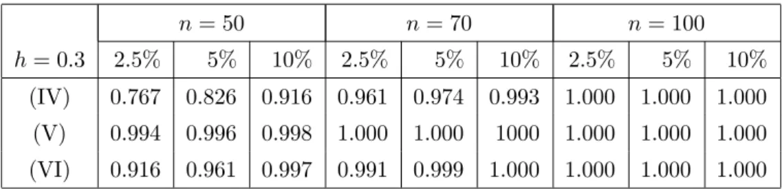
h= 0.3 2.5% 5% 10% 2.5% 5% 10% 2.5% 5% 10% (IV) 0.767 0.826 0.916 0.961 0.974 0.993 1.000 1.000 1.000 (V) 0.994 0.996 0.998 1.000 1.000 1000 1.000 1.000 1.000 (VI) 0.916 0.961 0.997 0.991 0.999 1.000 1.000 1.000 1.000

Table 4.3. Simulated rejection probabilities of the bootstrap test with bandwidth h= 0.3 for the regression and variance functions in (4.4). The error has a standard normal distribution and the explanatory variable X has a uniform distribution on the interval [0,1].

n= 50 n= 70 n= 100

h= 0.5 2.5% 5% 10% 2.5% 5% 10% 2.5% 5% 10% (IV) 0.718 0.811 0.902 0.943 0.968 0.996 1.000 1.000 1.000 (V) 0.989 0.991 0.999 1.000 1.000 1.000 1.000 1.000 1.000 (VI) 0.902 0.950 0.999 0.987 0.992 1.000 1.000 1.000 1.000

Table 4.4. Simulated rejection probabilities of the bootstrap test with bandwidth h= 0.5 for the regression and variance functions in (4.4). The error has a standard normal distribution and the explanatory variable X has a uniform distribution on the interval [0,1].

Example 4.2. Our second example refers to the work of Zhu, Fujikoshi and Naito (2001), who proposed functionals of a marked empirical process of the squared nonparametric residuals as test statistic in the problem of testing for homoscedasticity. In a simula-tion study they investigated the finite sample properties for the following regression and variance functions :

(IV) m(x) = 1 + 2x σ(x) = 0.25 +x

(V) m(x) = 1 + 2x σ(x) = 0.25 + 4(x₋0.25)2

(V I) m(x) = 1 + 2x σ(x) = 0.25 exp(xlog 5).

(4.4)

In Table 4.3 and 4.4 we display the rejection probabilities of the new Cram´er von Mises (bootstrap) test proposed in Section 3 for the sample sizes n = 50, n = 70 and n = 100. The two tables correspond again to the bandwidths h= 0.3 andh= 0.5, respectively. We observe no substantial differences between the two choices of the bandwidth. The results in the tables for sample size n= 50 and n= 70 and the 5% level are directly comparable with Table 2 in Zhu, Fujikoshi and Naito (2001). We observe that in model (IV) and (VI) the rejection probabilities of the test of Zhu, Fujikoshi and Naito (2001) are very similar

to those obtained by the new test. However, in model (V) the power of the new test is at least three times larger as the power of the test of Zhu, Fujikoshi and Naito (2001). Thus the new procedure performs reasonably well in the examples considered by these authors.

n= 50 n= 100 n= 200

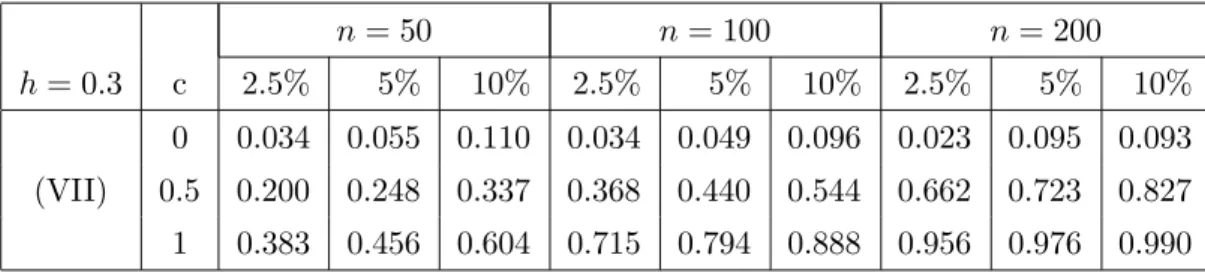
h= 0.3 c 2.5% 5% 10% 2.5% 5% 10% 2.5% 5% 10% 0 0.034 0.055 0.110 0.034 0.049 0.096 0.023 0.095 0.093 (VII) 0.5 0.200 0.248 0.337 0.368 0.440 0.544 0.662 0.723 0.827 1 0.383 0.456 0.604 0.715 0.794 0.888 0.956 0.976 0.990

Table 4.5. Simulated rejection probabilities of the bootstrap test with bandwidth h = 0.3 for the one-parametric hypothesis (4.5). The regression and variance functions are given by (4.6), the error has a standard normal distribution and the explanatory variable X has a uniform distribution on the interval [0,1].

n= 50 n= 100 n= 200

h= 0.5 c 2.5% 5% 10% 2.5% 5% 10% 2.5% 5% 10% 0 0.025 0.042 0.087 0.021 0.043 0.089 0.021 0.046 0.087 (VII) 0.5 0.167 0.218 0.304 0.262 0.321 0.416 0.417 0.473 0.586 1 0.348 0.424 0.578 0.690 0.752 0.821 0.919 0 .942 0.967

Table 4.6. Simulated rejection probabilities of the bootstrap test with bandwidth h = 0.5 for the one-parametric hypothesis (4.5). The regression and variance functions are given by (4.6), the error has a standard normal distribution and the explanatory variable X has a uniform distribution on the interval [0,1].

Example 4.3. Our final example considers the problem of testing for a one-parametric class of variance functions, that is

H0 :σ2(x) = 1 +θx2 (4.5)

for some θ∈IR. For this we simulate data according to the model

(V II) m(x) = 1 +x σ(x) = 1 + 3x2 _{+ 2.5csin(2πx) (4.6)}

where the case c= 0 corresponds to the null hypothesis and the choices c= 0.5,1 to two alternatives. The errors in model (1.1) are standard normal and the covariates follow again a uniform distribution on the interval [0,1]. The rejection probabilities of the Cram´er von

Mises test are displayed in Table 4.5 and 4.6 corresponding to the bandwidthsh= 0.3 and

h = 0.5, respectively. We observe a good approximation of the nominal level (for both choices of the bandwidth) and reasonable rejection probabilities under the two alternatives (c= 0.5,1). In this case the power of the test depends again sensitively on the choice of the bandwidth.

4.2

Data example

We consider data on (log of) concentration of sulfate in rain at two towns (Coweeta and Lewiston) in North Carolina. The data were previously analyzed by Hall and Hart (1990), in the context of bootstrap tests for nonparametric analysis of covariance, where the covariate is ‘amount of rainfall’. The sulfate concentration was available on a weekly basis over a five year period from 1979 to 1983. There were 220 weeks among all 261 weeks where data were available at Coweeta and 215 weeks where data were available at Lewiston. Hall and Hart (1990) restricted their analysis to the 189 weeks where data were available at both towns.

A crucial assumption in the applicability of their test for the comparison of two regression curves is a constant (not necessary equal) variance of the observations in both towns. In order to investigate whether this assumption is justified we applied the new bootstrap test to each data set, respectively. The bandwidth h was chosen by least squares cross validation, b = 500 bootstrap replications were used and we transformed the covariate (week) onto the interval [0,1] by dividing by 261. For the Lewiston data ap-value of 0.397 and for the Coweeta data ap-value of 0.418 were observed. Hence, Hall and Hart’s (1990) assumption of constant variability in both groups is strictly supported by our test.

Appendix : Proofs

In what follows _{k · k} denotes the Euclidean norm. For our main asymptotic results we require the following regularity conditions.

(A1) :

(i) As n_{→ ∞}: h_→0,nh4 _{→0 andnh}3+2δ_(logh−1₎−1 _{→ ∞ for someδ >0.}

(A2) :

(i) FX is three times continuously differentiable and infa≤x≤bfX(x)>0.

(ii) F0_{(y|x) exists, is continuous in (x, y) for all x and yand sup}

x,y|y2F0(y|x)|<∞, and

the same holds for all other partial derivatives of F(y_|x) with respect to x and y up to order two.

(iii)m(x) is twice continuously differentiable.

(iv)All partial derivatives up to order three ofσ2

θ(x) with respect toxand the components

of θ exist and are continuous in (x, θ) for all x and θ. Moreover, infa≤x≤bσ(x)>0.

(v)E(ε4_)<∞.

(A3) :

(i) Θ is a compact subspace of IRp.

(ii) θ0 is an interior point of Θ.

(iii)For all ε >0, inf_kθ−θ0k>εE[(σ 2

θ(X)−σθ20(X)) 2_]>0.

(iv) The matrix Ω defined in (3.2) is non-singular.

(A4) : E[r2_{(X)]<∞ and r(x) is twice continuously differentiable for all x.}

A.1

Proof of Lemma 2.1.

The necessary part follows from (2.7). In order to show that the equality of the distribu-tions of the random variables is also sufficient for the hypothesis σ2 _{∈ M={σ}2

θ |θ ∈Θ},

we note that it follows from (2.7) that

E[ε2n_{] =E[ε}2n 0 ] =E h_σ2_(X) σ2 ˜ θ0(X) ε2ni_=E[ε2n_]Ehσ2(X) σ2 ˜ θ0(X) ni

for all n ∈IN, which implies that

Ehσ 2_(X) σ2 ˜ θ0(X) ni = 1

for all n _∈ IN. Therefore we obtain from Carleman’s condition [see e.g. Feller (1966) p. 228] that the distribution of the random variable σ2_(X)/σ2

˜

θ0(X) coincides with the

distribution of the constant random variable U _≡1, that is σ2 _{∈ M={σ}2

A.2

Proof of Theorem 3.1 and 3.4.

The proof requires several auxiliary results.

Lemma A.1 If the assumptions of Theorem 3.1 are satisfied, then the following stochastic expansion is valid : Z σ−2(x)[ˆσ2(x)−σ2(x)]dFX(x) =n−1 n X i=1 σ−2(Xi)[{Yi−m(Xi)}2−σ2(Xi)] +oP(n−1/2).

Proof. With the notation Kh(·) =h−1K(·/h) we obtain the decomposition Z σ−2(x)ˆσ2(x)dFX(x) = n−1 n X i=1 Z Kh(x−Xi) ˆfX−1(x)σ−2(x)dFX(x)Yi2 −2n−1 n X i=1 Z Kh(x−Xi) ˆfX−1(x)σ−2(x)dFX(x)Yimˆ(Xi) +n−1 n X i=1 Z Kh(x−Xi) ˆfX−1(x)σ−2(x)dFX(x) ˆm2(Xi) = T1+T2+T3, (A.1)

where the last equality defines the random variables T1, T2, T3. For the first term T1 in

(A.1) we have T1 = n−1 n X i=1 Z Kh(x−Xi)σ−2(x)[Yi2−E(Y2|X =x)]dx +n−1 n X i=1 Z Kh(x−Xi)[fX(x)−fˆX(x)] ˆfX−1(x)σ−2(x)[Yi2−E(Y2|X=x)]dx + Z σ−2(x)E(Y2|X=x)dFX(x) = n−1 n X i=1 σ−2(Xi)[Yi2 −E(Yi2|Xi)] +E[σ−2(X)E(Y2|X)] +oP(n−1/2). (A.2)

Using a similar decomposition as for T1 we obtain

T2 = −2n−1 n X i=1 σ−2(Xi)Yi[ ˆm(Xi)−E{mˆ(Xi)|X}] −2n−1 n X i=1 Z Kh(x−Xi) ˆfX−1(x)σ−2(x)dFX(x)YiE{mˆ(Xi)|X}+oP(n−1/2) = T2,1+T2,2, (A.3)

where the last line defines the random variables T2,i (i = 1,2) and X = (X1, . . . , Xn) is

the vector of covariates. The second term on the right hand side of (A.3) equals (using again a similar derivation as for the stochastic expansion ofT1)

T2,2 = − 2 n n X i=1 Z Kh(x−Xi) ˆfX−1(x)σ−2(x)dFX(x)Yim(Xi) +oP(n−1/2) = ₋2 n n X i=1 σ−2(Xi)[Yim(Xi)−m2(Xi)]−2E[σ−2(X)m2(X)] +oP(n−1/2), (A.4)

whereas the first term can be written as

T2,1 = − 2 n2 n X i=1 n X j=1 Kh(Xi−Xj)fX−1(Xi)σ−2(Xi)Yi(Yj −m(Xj)) +oP(n−1/2) = 1 n2 n X i=1 n X j=1 Unij +oP(n−1/2),

where the random variables Unij are defined by

Unij =−2Kh(Xi−Xj)fX−1(Xi)σ−2(Xi)Yi(Yj −m(Xj)).

Now a standard argument shows that

T2,1 = n−2 n X i=1 n X j=1

[Unij−E{Unij|Xi, Yi} −E{Unij|Xj, Yj}+E{Unij}]

+n−1 n X i=1 E{Uni1|Xi, Yi}+n−1 n X j=1 E{Un1j|Xj, Yj} −n−2 n X i=1 n X j=1 E{Unij} +oP(n−1/2) = 4 X k=1 Ank+oP(n−1/2), (A.5)

where the last line defines the random variables Ank (k = 1, . . . ,4). For An1, note that

E[An1] = 0 and hence, by Chebyshev’s inequality, for any K >0,

P(_|An1|> Kn−1E{Un∗12(Un∗12+Un∗21)}1/2) (A.6) ≤K−2_n2_E{U∗ n12(Un∗12+Un∗21)}−1E(A2n1) =K−2n−2E_{U_n∗₁₂(U_n∗₁₂+U_n∗₂₁)_}−1X i,j X l,m E(U_nij∗ U_nlm∗ ),

where U_nij∗ = Unij −E{Unij|Xi, Yi} −E{Unij|Xj, Yj}+E{Unij}. Since E[Unij∗ ] = 0, the

either i orj equals l orm and the other differs from l and m, are also zero, because, for example when i=l and j ₆=m,

E[U_nij∗ E_{U_nim∗ _|Xi, Yi, Xj, Yj}] = 0.

Thus, only the 2n2 _{terms for which (i, j) equals (l, m) or (m, l) are non-zero. Hence,}

(A.6) is bounded by K−2_{, which can be made arbitrarily small for K large enough. It}

now follows that An1 =OP(n−1h−1/2) =oP(n−1/2), since it is easily seen that

E_{U_n∗₁₂(U_n∗₁₂+U_n∗₂₁)_}=O(h−1).

Next, note that An2 =An4 = 0, and that

An3 =−2n−1 n X i=1 σ−2_(X i)m(Xi)(Yi−m(Xi)) +oP(n−1/2).

Hence it follows from (A.3)

T2 = − 4 n n X i=1 σ−2(Xi)m(Xi)[Yi−m(Xi)]−2E[σ−2(X)m2(X)] +oP(n−1/2). (A.7)

It remains to consider the term T3 in the decomposition (A.1), for which a similar

argu-ment as used for the stochastic expansion of the term T1 yields

T3 = n−1 n X i=1 Z Kh(x−Xi)σ−2(x)[ ˆm2(Xi)−E{mˆ(Xi)|X}2]dx (A.8) +n−1 n X i=1 Z Kh(x−Xi) ˆfX−1(x)σ−2(x)E{mˆ(Xi)|X}2dFX(x) +oP(n−1/2).

The second term of (A.8) can be written as E[σ−2(X)m2(X)] +oP(n−1/2), whereas the

first term equals (using similar techniques as for the stochastic expansion of the termT2,1)

n−3 n X i=1 n X j=1 n X k=1 Kh(Xi−Xj)Kh(Xi−Xk)fX−2(Xi)σ−2(Xi)[YjYk−m(Xj)m(Xk)] +oP(n−1/2) = 2n−1 n X i=1 σ−2(Xi)m(Xi)[Yi−m(Xi)] +oP(n−1/2). (A.9)

It now follows from (A.1), (A.2), (A.7) and (A.9) that

Z σ−2(x)ˆσ2(x)dFX(x) =n−1 n X i=1 σ−2(Xi)[Yi2−E(Yi2|Xi)] +E[σ−2(X)E(Y2|X)]

−2n−1 n X i=1 σ−2(Xi)m(Xi)[Yi−m(Xi)]−E[σ−2(X)m2(X)] +oP(n−1/2) =n−1 n X i=1 σ−2(Xi)[Yi2−E(Y2|Xi)−2m(Xi){Yi−m(Xi)}+σ2(Xi)] +oP(n−1/2) =n−1 n X i=1 σ−2(Xi)[Yi−m(Xi)]2+oP(n−1/2). 2

Lemma A.2 If the assumptions of Theorem 3.1 are satisfied, then under the null hypoth-esis H0,

ˆ

θ−θ0 →P 0.

Proof. Recall the definition Sn in (2.11) and define

S0(θ) =E{σθ40(X)}E(ε 4

−1) +E_{[σ_θ2(X)₋σ_θ2₀(X)]2_}, (A.10) It follows from Theorem 5.7 in van der Vaart (1998, p. 45) that it suffices to show that

sup θ | Sn(θ)−S0(θ)| →P 0 inf kθ−θ0k>ε S0(θ)> S0(θ0)∀ε >0.

The latter follows from assumption (A3)(iii), whereas for the former, note that sup θ | Sn(θ)−S0(θ)| ≤sup θ | Sn(θ)−S˜n(θ)|+ sup θ | ˜ Sn(θ)−S0(θ)|, (A.11)

where the random variable ˜Sn is given by

˜ Sn(θ) =n−1 n X i=1 [(Yi−m(Xi))2−σθ2(Xi)]2.

From the uniform consistency of ˆm(·) it follows that the first term on the right hand side of (A.11) is oP(1). For the second term, apply e.g. Theorem 2 in Jennrich (1969). 2

Lemma A.3 If the assumptions of Theorem 3.1 are satisfied, then under the null hypoth-esis H0, ˆ θ−θ0 = Ω−1n−1 n X i=1 [{Yi−m(Xi)}2−σ2(Xi)] ∂σ2 θ(Xi) ∂θ θ=θ0+oP(n −1/2_).

Proof. First note that ˆθ−θ0 =oP(1) by Lemma A.2. Hence, it follows from assumption

(A3)(ii) that ˆθ is an interior point of Θ for n large enough. Now write

∂Sn(θ) ∂θ _θ=ˆθ − ∂Sn(θ) ∂θ _θ=θ 0 = ∂2_S n(θ) ∂θ∂θ0 _θ=θ 1n(ˆθ−θ0),

for some θ1n between ˆθ and θ0. Then, we obtain that

ˆ θ₋θ0 =− ∂2_S n(θ) ∂θ∂θ0 _θ=θ 1n !−1 ∂Sn(θ) ∂θ _θ=θ 0, (A.12) where ∂Sn(θ) ∂θ _θ=θ 0=−2n −1Xn i=1 [(Yi−mˆ(Xi))2−σ2θ0(Xi)] ∂σ2 θ(Xi) ∂θ _θ=θ 0. (A.13)

In order to prove that ˆm(Xi) can be replaced by m(Xi) in the above expression, we can

follow the same type of arguments as presented in the proof of Lemma A.1, the main difference being that the weights are now all equal to n−1_{. It can be shown in this way}

that the left hand side of (A.13) equals

∂Sn(θ) ∂θ θ=θ0 = −2n −1Xn i=1 [(Yi−m(Xi))2−σθ20(Xi)] ∂σ2 θ(Xi) ∂θ θ=θ0+oP(n −1/2_).

Finally, we obtain from the continuity of ∂σ2θ

∂θ∂θ0 and Lemma A.2,

∂2_S n(θ) ∂θ∂θ0 _θ=θ 1n = 2 n n X i=1 ∂σ2 θ(Xi) ∂θ _θ=θ 1n ∂σ2 θ(Xi) ∂θ _θ=θ 1n !₀ − 2 n n X i=1 [(Yi−mˆ(Xi))2−σθ21n(Xi)] ∂2_σ2 θ(Xi) ∂θ∂θ0 _θ=θ 1n = 2 n n X i=1 ∂σ2 θ(Xi) ∂θ _θ=θ 0 ∂σ2 θ(Xi) ∂θ _θ=θ 0 !0 − 2 n n X i=1 [(Yi−m(Xi))2−σ2θ0(Xi)] ∂2_σ2 θ(Xi) ∂θ∂θ0 _θ=θ 0 +oP(1) = 2Ω +oP(1),

and the assertion of Lemma A.3 follows. 2

Proof of Theorem 3.1. From the proof of Theorem 1 in Akritas and Van Keilegom (2001) (hereafter called AVK) it follows that

ˆ Fε(y)−Fε(y) =n−1 n X i=1 I(εi ≤y)−Fε(y) (A.14) +fε(y) Z σ−1(x)[y{σˆ(x)−σ(x)}+ ˆm(x)−m(x)]dFX(x) +Rn1(y),

where

sup

y∈IR

|Rn1(y)|=oP(n−1/2).

Note that AVK assume that the regression function m and the variance function σ2 _are

L-functionals that depend on a certain score function, say J. It is easy to show that the representation (A.14) can be extended to the choiceJ ≡1, which leads to the conditional mean and variance that we consider in this paper (it suffices to replace Propositions 3–5 in AVK by their analogues for the estimators of the conditional mean and variance). We will now construct a similar representation for the differences ˆFε0(y)−Fε(y). We will

do this by showing that Theorem 1 in AVK can be adapted to the case where ˆσ(x) is replaced by ˆσ0(x). It can be easily seen that Propositions 3–5 in AVK continue to hold true

when ˆσ is replaced by ˆσ0 (use assumption (A2)(iv) and the fact that ˆθ−θ0 =OP(n−1/2)).

We can now follow exactly the same derivation as for the above representation, and find in this way that

ˆ Fε0(y)−Fε(y) = n−1 n X i=1 I(εi ≤y)−Fε(y) (A.15) + fε(y) Z σ−1(x)[y{σˆ0(x)−σ(x)}+ ˆm(x)−m(x)]dFX(x) +Rn2(y), where sup y∈IR |Rn2(y)|=oP(n−1/2).

Hence, under the null hypothesis we obtain ˆ Fε(y)−Fˆε0(y) =yfε(y) Z σ−1(x)[ˆσ(x)−σˆ0(x)]dFX(x) +oP(n−1/2) =yfε(y) 2 Z σ−2(x)[ˆσ2(x)₋σˆ₀2(x)]dFX(x) +oP(n−1/2) (A.16)

uniformly in y. On the other hand it follows from Lemma A.1 that

Z σ−2(x)[ˆσ2(x)₋σ2(x)]dFX(x) =n−1 n X i=1 σ−2(Xi)[{Yi−m(Xi)}2−σ2(Xi)] +oP(n−1/2), (A.17)

whereas Lemma A.3 and a Taylor expansion yield

Z σ−2(x)[ˆσ₀2(x)₋σ2(x)]dFX(x) =n−1 n X i=1 Z σ−2(x)Kh(x−Xi){σ_θˆ2(x)−σ2θ0(x)}dx+oP(n −1/2₎

=n−1 n X i=1 σ−2(Xi){σ_θ2ˆ(Xi)−σθ20(Xi)}+oP(n −1/2₎ =n−1 n X i=1 σ−2(Xi) ∂σ2 θ(Xi) ∂θ _θ=θ 0 !0 Ω−1n−1 n X i=1 [_{Yi−m(Xi)}2−σ2(Xi)] ∂σ2 θ(Xi) ∂θ _θ=θ 0 +oP(n−1/2) = Z σ−2(x) ∂σ 2 θ(x) ∂θ _θ=θ 0 !0 dFX(x) Ω−1n−1 n X i=1 [_{Yi−m(Xi)}2−σ2(Xi)] ∂σ2 θ(Xi) ∂θ _θ=θ 0 +oP(n−1/2). (A.18)

The assertion of Theorem 3.1 now follows from (A.16) - (A.18). 2

Proof of Theorem 3.4. In a similar way as in the proof of Lemmas A.1 and A.2 in Van Keilegom, Gonz´alez-Manteiga and S´anchez-Sellero (2005), it can be shown that under the alternative hypothesis H1,

ˆ θ−θ0 = Ω−1n−1 n X i=1 [{Yi−m(Xi)}2−σ_θ2˜_0n(Xi)] ∂σ2 θ(Xi) ∂θ _θ=˜θ 0n +Ω−1n−1/2 Z r(x)∂σ 2 θ(x) ∂θ θ=θ0dFX(x) +oP(n −1/2_), where ˜ θ0n = argmin θ∈Θ E[{(Y −m(X)) 2_−σ2 θ(X)}2] = argmin θ∈Θ E[_{σ2(X)₋σ_θ2(X)_}2].

The proof parallels that of Theorem 3.1, except for the term considered in (A.18). For this expression we obtain under local alternatives

Z σ−2(x)[ˆσ₀2(x)−σ2(x)]dFX(x) = Z σ_θ−₀2(x)∂σ 2 θ(x) ∂θ _θ=θ 0 0 dFX(x)Ω−1n−1 n X i=1 [_{Yi−m(Xi)}2−σ2_θ˜_0n(Xi)] ∂σ2 θ(Xi) ∂θ _θ=˜θ 0n + Z σ−_θ02(x)∂σ 2 θ(x) ∂θ _θ=θ 0 0 dFX(x)Ω−1n−1/2 Z r(x)∂σ 2 θ(x) ∂θ _θ=θ 0dFX(x) −n−1/2 Z σ_θ−₀2(x)r(x)dFX(x) +oP(n−1/2).

It is easy to show that the asymptotic distribution of the random variable

n−1 n X i=1 [{Yi−m(Xi)}2−σ_θ2˜_0n(Xi)] ∂σ2 θ(Xi) ∂θ |θ=˜θ0n

under H1 equals the asymptotic distribution of n−1 n X i=1 [_{Yi−m(Xi)}2−σθ20(Xi)] ∂σ2 θ(Xi) ∂θ |θ=θ0

underH0.The rest of the proof is similar as in the proofs of Theorem 3.1 and Corollaries

3.2 and 3.3. Hence, the assertion of Theorem 3.4 follows. 2

References

Akritas, M.G. and Van Keilegom, I. (2001). Nonparametric estimation of the residual distribution. Scand. J. Statist., 28, 549–568.

Atkinson, A. C. (1985). Plots, transformations and regression : an introduction to graph-ical methods of diagnostic. Oxford : Clarendon Pr.

Breusch, T.S. and Pagan , A.R. (1979). A simple test for heteroscedasticity and random coefficient variation. Econometrika,47, 1287–1294.

Carroll, R. and Ruppert, D. (1988). Transformation and weighting in regression. Mono-graphs on Statistics and Applied Probability. New York, Chapman and Hall.

Cook, R.D. and Weisberg, S. (1983). Diagnostics for heteroscedasticity in regression.

Biometrika, 70, 1–10.

Dette, H. and Munk, A. (1998). Testing heteroscedasticity in nonparametric regression.

J. R. Statist. Soc. B,60, 693–708.

Dette, H. (2002). A consistent test for heteroscedasticity in nonparametric regression based on the kernel method. J. Statist. Planning Infer.,103, 311–329.

Diblasi, A. and Bowman, A. (1997). Testing for constant variance in a linear model.

Statist. Probab. Lett.,33, 95–103.

Eubank, R.L. and Thomas, W. (1993). Detecting Heteroscedasticity in Nonparametric Regression. J. Roy. Statist. Soc. Ser. B,55, 145–155.

Fan, Y.,and Linton, O. (2003). Some higher-order theory for a consistent non-parametric model specification test. J. Stat. Plann. Inference 109, 125-154.

Feller, W. (1966). An introduction to probability theory and its applications. Vol II.Wiley Series in Probability and Mathematical Statistics. New York.

Francisco-Fern´andez, M. and Vilar-Fern´andez, J.M. (2005). Two tests for heteroscedas-ticity in nonparametric regression. Technical Report, Universidad de A Coru˜na. Hall, P. and Hart, J.D. (1990). Bootstrap test for difference between means in

Harrison, M.J. and McCabe, B.P.M. (1979). A test for heteroscedasticity based on least squares residuals. J. Amer. Statist. Assoc., 74, 494–500.

Jennrich, R.I. (1969). Asymptotic properties of non-linear least-squares estimators. Ann. Math. Statist.,40, 633–643.

Koenker, R. and Bassett, G. (1981). Robust tests for heteroscedasticity based on regres-sion quantiles. Econometrika, 50, 43–61.

Liero, H. (2003). Testing homoscedasticity in nonparametric regression. J. Nonpar. Statist., 15, 31–51.

M¨uller, H.G. and Stadtm¨uller, U. (1987). Estimation of heteroscedasticity in regression analysis. Ann. Statist., 15, 610–625.

Nadaraya, E.A. (1964). On estimating regression. Theory Probab. Appl., 15, 134–137. Rice, J. (1984). Bandwidth choice for nonparametric regression. Ann. Statist., 12, 1215–

1230.

van der Vaart, A.W. (1998). Asymptotic statistics. Cambridge Univ. Press. Cambridge. Van Keilegom, I. and Veraverbeke, N. (2002). Density and hazard estimation in censored

regression models. Bernoulli,8, 607–625.

Van Keilegom , I., Gonz´alez-Manteiga, W. and S´anchez-Sellero, C. (2005). Goodness-of-fit tests in parametric regression based on the estimation of the error distribu-tion. Discussion Paper 0405, Institute of Statistics, Universit´e catholique de Louvain

(http://www.stat.ucl.ac.be/ISpub/ISdp.html).

Watson, G.S. (1964). Smooth regression analysis. Sankhy¯a, Ser. A, 26, 359–372.

Zhu, L., Fujikoshi, Y. and Naito, K. (2001). Heteroscedasticity checks for regression models. Science in China (Series A), 44, 1236–1252.