Bounds on the Sample Complexity for Private Learning and Private Data Release

(1)

Bounds on the Sample Complexity for Private Learning and Private

Data Release

∗

Amos Beimel† Hai Brenner‡ Shiva Prasad Kasiviswanathan§ Kobbi Nissim¶ June 28, 2013

Abstract

Learning is a task that generalizes many of the analyses that are applied to collections of data, in particular, to collections of sensitive individual information. Hence, it is natural to ask what can be learned while preserving individual privacy. [Kasiviswanathan, Lee, Nissim, Raskhodnikova, and Smith; FOCS 2008] initiated such a discussion. They formalized the notion ofprivate learning, as a combination of PAC learning and differential privacy, and investigated what concept classes can be learned privately. Somewhat surprisingly, they showed that for finite, discrete domains (ignoring time complexity), every PAC learning task could be performed privately with polynomially many labeled examples; in many natural cases this could even be done in polynomial time.

While these results seem to equate non-private and private learning, there is still a significant gap: the sample complexity of (non-private) PAC learning is crisply characterized in terms of the VC-dimension of the concept class, whereas this relationship is lost in the constructions of private learners, which exhibit, generally, a higher sample complexity.

Looking into this gap, we examine several private learning tasks and give tight bounds on their sample complexity. In particular, we show strong separations between sample complexities of proper and improper private learners (such separation does not exist for non-private learners), and between sample complexities of efficient and inefficient proper private learners. Our results show that VC-dimension is not the right measure for characterizing the sample complexity of proper private learning.

We also examine the task of private data release(as initiated by [Blum, Ligett, and Roth; STOC 2008]), and give new lower bounds on the sample complexity. Our results show that the logarithmic dependence on size of the instance space is essential for private data release.

Key Words. Differential privacy, PAC learning, Sample complexity, Private data release.

∗

A preliminary version of this work appeared in the 7th Theory of Cryptography Conference, TCC 2010 [1]. †

Dept. of Computer Science, Ben-Gurion University. [email protected]. Partially supported by the Israel Science Foundation (grant No. 938/09) and by the Frankel Center for Computer Science at BGU.

‡

Dept. of Mathematics, Ben-Gurion University. [email protected]. §

General Electric Research Center. [email protected]. Part of this wok was done while the author was a postdoc at Los Alamos National Laboratory and IBM T.J. Watson Research Center.

¶

Dept. of Computer Science, Ben-Gurion University. [email protected]. Research partly supported by the Israel Science Foundation (grant No. 860/06).

(2)

1 Introduction

Consider a scenario in which a survey is conducted among a sample of random individuals and data mining techniques are applied to learn information on the entire population. If such information will disclose information on the individuals participating in the survey, then they will be reluctant to participate in the survey. To address this question, Kasiviswanathan et al. [19] introduced the notion of private learning, where a private learner is required to output a hypothesis that gives accurate classification while protecting the privacy of the individual samples from which the hypothesis was obtained.

The definition of a private learner is a combination of two qualitatively different notions. One is that of probably approximately correct (PAC) learning [26], the other of differential privacy [13]. PAC learning, on one hand, is an average case requirement, which requires that the output of the learner on most samples is good. Differential privacy, on the other hand, is a worst-case

requirement. It is a strong notion of privacy that provides meaningful guarantees in the presents of powerful attackers and is increasingly accepted as a standard for providing rigorous privacy. Recent research on privacy has shown, somewhat surprisingly, that it is possible to design differentially private variants of many analyses. Further discussions on differential privacy can be found in the surveys of Dwork [11, 12].

We next give more details on PAC learning and differential privacy. In PAC learning, a collec-tion of samples (labeled examples) is generalized into a hypothesis. It is assumed that the examples are generated by sampling from some (unknown) distribution D and are labeled according to an (unknown) concept c taken from some concept class C. The learned hypothesis h should predict with high accuracy the labeling of examples taken from the distribution D, an average-case re-quirement. In differential privacy the output of a learner should not be significantly affected if a particular example is replaced with an arbitrary example. Concretely, differential privacy considers the collection of samples as a database, defines that two databases are neighbors if they differ in exactly one sample, and requires that for every two neighboring databases the output distribution of a private learner should be similar.

In this paper, we consider private learning of finite, discrete domains. Finite domains are natural as computers only store information with finite precision. The work of [19] demonstrated that private learning in such domains is feasible – any concept class that is PAC learnable can be learned privately (but not necessarily efficiently), by a “private Occam’s razor” algorithm, with sample complexity that is logarithmic in the size of the hypothesis class.1 Furthermore, taking into account the earlier result of [3] (that all concept classes that can be efficiently learned in the

statistical queries model can be learned privately and efficiently) and the efficient private parity learner of [19], we get that most “natural” computational learning tasks can be performed privately and efficiently (i.e., with polynomial resources). This is important as learning problems generalize many of the computations performed by analysts over collections of sensitive data.

The results of [3, 19] show that private learning is feasible in an extremely broad sense, and hence, one can essentially equate learning and private learning. However, the costs of the private learners constructed in [3, 19] are generally higher than those of non-private ones by factors that depend not only on the privacy, accuracy, and confidence parameters of the private learner. In particular, the well-known relationship between the sample complexity of PAC learners and the VC-dimension of the concept class (ignoring computational efficiency) [6] does not hold for the above

(4)

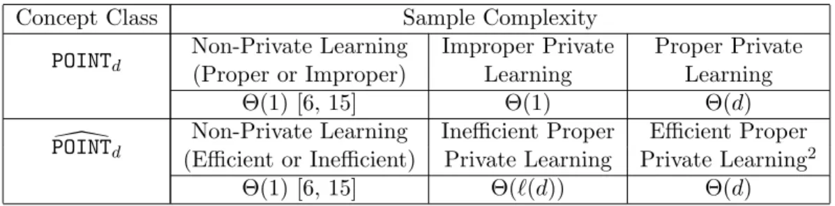
Concept Class Sample Complexity

POINTd

Non-Private Learning Improper Private Proper Private (Proper or Improper) Learning Learning

Θ(1) [6, 15] Θ(1) Θ(d)

\

POINTd

Non-Private Learning Inefficient Proper Efficient Proper (Efficient or Inefficient) Private Learning Private Learning2

Θ(1) [6, 15] Θ(`(d)) Θ(d)

Table 1: Our separation results (ignoring dependence on , α, β), where `(d) is any function that grows asω(logd).

constructions of private learners; the sample complexity of the algorithms of [3, 19] is proportional to the logarithm of the size of the concept class. Recall that the VC-dimension of a concept class is bounded by the logarithm of its size, and is significantly lower for many interesting concept classes, hence, there may exist learning tasks for which “very practical” non-private learner exists, but any private learner is “impractical” (with respect to the sample size required).

The focus of this work is on a fine-grain examination of the differences in complexity between private and non-private learning. The hope is that such an examination will eventually lead to an understanding of which complexity measure is relevant for the sample complexity of private learning, similar to the well-understood relationship between the VC-dimension and sample complexity of PAC learning. Such an examination is interesting also for other tasks, and a second task we examine is that of releasing a sanitization of a data set that simultaneously protects privacy of individual contributors and offers utility to the data analyst. See the discussion in Section 1.1.2.

1.1 Our Contributions

We now give a brief account of our results. Throughout this rather informal discussion we will treat the accuracy, confidence, and privacy parameters as constants (a detailed analysis revealing the dependency on these parameters is presented in the technical sections). We use the term “efficient” for polynomial time computations.

Following standard computational learning terminology, we will call learners for a concept class

C that only output hypotheses in C proper, and other learners improper. The original motivation in computational learning theory for this distinction is that there exist concept classesC for which proper learning is computationally intractable [25], whereas it is tractable to learnCimproperly [26]. As we will see below, the distinction between proper and improper learning is useful also when discussing private learning, and for reasons other than making intractable learning tasks tractable. Our results on private learning are summarized in Table 1.

1.1.1 Proper and Improper Private Learning

It is instructive to look into the construction of the private Occam’s razor algorithm of [19] and see why its sample complexity is proportional to the logarithm of the size of the hypothesis class used. The algorithm uses the exponential mechanism of McSherry and Talwar [23] to choose a hypothesis. The choice is probabilistic, where the probability mass that is assigned to each of the

(5)

hypotheses decreases exponentially with the number of samples that are inconsistent with it. A union-bound argument is used in the claim that the construction actually yields a learner, and a sample size that is logarithmic in the size of the hypothesis class is needed for the argument to go through. The question is whether such sample size is required?

To address the above question, we consider a simple, but natural, class POINT = {POINTd}

containing the conceptscj :{0,1}d→ {0,1} wherecj(x) = 1 for x=j, and 0 otherwise. The

VC-dimension ofPOINTd is one, and hence, it can be learned (non-privately and efficiently, properly or

improperly) with merely O(1) samples.

In sharp contrast, (when used for properly learning POINTd) the above-mentioned private

Oc-cam’s razor algorithm from [19] requiresO(log(|POINTd|)) =O(d) samples – obtaining the largest

possible gap in sample complexity when compared to non-private learners! Our first result is a matching lower bound. We prove that any proper private learner for POINTd must use Ω(d)

sam-ples, therefore, answering negatively the question (from [19]) of whether proper private learners should exhibit sample complexity that is approximately the VC-dimension (or even a function of the VC-dimension) of the concept class.3

A natural way to improve the sample complexity is to use the private Occam’s razor to improp-erly learnPOINTdwith a smaller hypothesis class that is still expressive enough forPOINTd, reducing

the sample complexity to the logarithm of the smaller hypothesis class. We show that this indeed is possible, as there exists a hypothesis class of size O(d) that can be used for learning POINTd

improperly, yielding an algorithm with sample complexity O(logd). Furthermore, this bound is tight, any hypothesis class for learning POINTd must contain Ω(d) hypotheses. These bounds are

interesting as they give a separation between proper and improper private learning – proper pri-vate learning ofPOINTdrequires Ω(d) samples, whereasPOINTdcan be improperly privately learned

using O(logd) samples. Note that such a combinatorial separation does not exist for non-private learning, as VC-dimension number of samples are needed and sufficient for both proper and im-proper non-private learners. Furthermore, the Ω(d) lower bound on the size of the hypothesis class maps a clear boundary to what can be achieved in terms of sample complexity using the private Occam’s razor for POINTd. It might even suggest that any private learner for POINTd should use

Ω(logd) samples.

It turns out, however, that the intuition expressed in the last sentence is at fault. We construct an efficient improper private learner forPOINTd that uses merelyO(1) samples, hence, establishing

the strongest possible separation between proper and improper private learners. For the construc-tion, we extrapolate on a technique from the efficient private parity learner of [19]. The construction of [19] utilizes a natural non-private proper learner, and hence, results in a proper private learner. Due to the bounds mentioned above, we cannot use a proper learner for POINTd, and hence, we

construct an improper (rather unnatural) learner to base our construction upon. Our construction utilizes a double-exponential hypothesis class, and hence, is inefficient (even outputting a hypoth-esis requires super-polynomial time). We use a simple compression using pseudorandom functions (akin to [24]) to make the algorithm efficient.

The above two improper learning algorithms use “heavy” hypotheses, that is, the hypotheses are Boolean functions that return 1 on many inputs (in contrast to a point function that returns 1 on exactly one input). Informally, each such heavy hypothesis protects the privacy since it could have been returned on many different concepts. The main technical point in these algorithms is

3_{Our proof technique yields lower bounds not only on private learning}_POINT

dproperly, but on private learning of

(6)

how to choose a heavy hypothesis with a small error. To complete the picture, we prove that using heavy hypotheses is unavoidable: Every private learning algorithm forPOINTdthat uses o(d)

samples must use heavy hypotheses.

Next we look into the concept class INTERVAL = {INTERVALd}, where for T = 2d we define

INTERVALd = {c1, . . . , cT+1} and, for 1 ≤ j ≤ T + 1, the concept cj : {1, . . . , T+ 1} → {0,1} is

defined as follows: cj(x) = 1 for x < j and cj(x) = 0 otherwise. As with POINTd, it is easy to

show that the sample complexity of any proper private learner for INTERVALd is Ω(d). We give

two results regarding the sample complexity of improper private learning of INTERVALd. The first

result shows that if a sublinear (ind) sample complexity private learner exists forINTERVALd, then

it must output, with high probability, a very “complex looking” hypothesis in the sense that the hypothesis must switch from zero to one (and vice-versa) exponentially many times, unlike any conceptcj ∈INTERVALdthat switches only once from one to zero atj. The second result considers

a generalization of the technique that yielded theO(1) sample improper private learner forPOINTd,

and shows that it alone would not yield a private learner forINTERVALdwith sublinear (ind) sample

complexity.

We apply the above lower bound on the number of samples for proper private learning POINTd

to show a separation in the sample complexity of efficient proper private learners (under a slightly relaxed definition of proper learning) and inefficient proper private learners. More concretely, assuming the existence of a pseudorandom generator with exponential stretch, we present a concept classPOINT\d– a subset ofPOINTd– such that every efficient private learner that learnsPOINT\dusing

POINTdrequires Ω(d) samples. In contrast, an inefficient proper private learner exists that uses only

a super-logarithmic number of samples. This is the first example in private learning where requiring efficiency on top of privacy comes at a price of larger sample size.

1.1.2 The Sample Size of Non-Interactive Sanitization Mechanisms

Given a database containing a collection of individual information, a sanitization is a release of information that protects the privacy of the individual contributors while offering utility to the analyst using the database. The setting is non-interactive if once the sanitization is released, then the original database and the curator play no further role. Blumet al.[4] presented a construction of such non-interactive sanitizers for count queries. LetC be a concept class consisting of efficiently computable predicates from a discretized domain X to{0,1}. Given a collectionD of data items taken fromX, Blumet al.employ the exponential mechanism [23] to (inefficiently) obtain another collection D0 with data items from X such that D0 maintains approximately correct count of

P

d∈Dc(d) for all concepts c ∈ C provided that the size of D is O(log(|X|)·VCDIM(C)). As

D0 is generated using the exponential mechanism, the differential privacy of D is protected. The database D0 is referred to as a synthetic database as it contains data items drawn from the same universe (i.e., from X) as the original databaseD.

We provide a new lower bound for non-interactive sanitization mechanisms. We show that for

POINTdevery non-interactive sanitization mechanism that is useful4 forPOINTdrequires a database

of size Ω(d). This lower bound is tight as the sanitization mechanism of Blum et al. for POINTd

uses a database of sizeO(d·VCDIM(POINTd)) =O(d). Our lower bound holds even if the sanitized

output is an arbitrary data structure, i.e., not necessarily a synthetic database.

4_{Informally, a mechanism is useful for a concept class if for every input, the output of the mechanism maintains}

(7)

1.2 Related Work

The notion of PAC learning was introduced by Valiant [26]. The notion of differential privacy was introduced by Dwork et al. [13]. Private learning was introduced in Kasiviswanathan et al. [19]. Beyond proving that (ignoring computation) every concept class with finite, discrete domain can be PAC learned privately (see Theorem 3.2 below), Kasiviswanathan et al. proved an equivalence between learning in the statistical queries model and private learning in the local communication model (a.k.a. randomized response). The general private data release mechanism we mentioned above was introduced in [4] along with a specific construction for halfspace queries. Also as men-tioned above, both [19] and [4] use the exponential mechanism of [23], a generic construction of differential private analyses, which (in general) does not yield efficient algorithms.

A recent work of Dwork et al. [14] considered the complexity of non-interactive sanitization under two settings: (a) sanitized output is a synthetic database, and (b) sanitized output is some arbitrary data structure. For the task of sanitizing with a synthetic database they show a separation between efficient and inefficient sanitization mechanisms based on whether the size of the instance space and the size of the concept class is polynomial in a (security) parameter or not. For the task of sanitizing with an arbitrary data structure they show a tight connection between the complexity of sanitization and traitor tracing schemes used in cryptography. They leave the problem of separating efficient private and inefficient private learning open.

Following the preliminary version of our paper [1], Chaudhuri and Hsu [8] study the sample complexity for private learning infinite concept classes when the data is drawn from a continuous distribution. Using techniques very similar to ours, they show that, under these settings, there exists a simple concept class for which any proper learner that uses a finite number of examples and guarantees differential privacy, fails to satisfy accuracy guarantee for at least one unlabeled data distribution. This implies that the results of Kasiviswanathan et al. [19] do not extend to infinite hypothesis classes on continuous data distributions.

Chaudhuri and Hsu [8] also study learning algorithms that are only required to protect the privacy of the labels (and not necessary protect the privacy of the examples themselves). They prove upper bounds and lower bounds for this scenario. In particular, they prove a lower bound on the sample complexity using the doubling dimension of the disagreement metric of the hypothesis class with respect to the unlabeled data distribution. This result does not imply our results. For example, the class POINTd can be properly learned using O(1) samples while protecting the

privacy of the labels, while we prove that Ω(d) samples are required to properly learn this class while protecting the privacy of the examples and the labels. It seems that label privacy may give enough protection in the restricted setting where the content of the underlying examples is publicly known. However, in many settings this information is highly sensitive. For example, in a database containing medical records we wish to protect the identity of the people in the sample (i.e., we do not want to disclose that they have been to a hospital).

It is well known that for all concept classes C, every learner for C requires Ω(VCDIM(C)) samples [15]. This lower bound on the sample size also holds for private learning. Blum, Ligett, and Roth [5] show that this result extends to the setting of private data release. They show that for all concept classes C, every non-interactive sanitization mechanism that is useful for C requires Ω(VCDIM(C)) samples (remember that the best upper bound is O(log(|X|)·VCDIM(C))). We show in Section 7 that the lower bound of Ω(VCDIM(C)) is not tight – there exists a concept class

C of constant VC-dimension such that every non-interactive sanitization mechanism that is useful forC requires a much larger sample size.

(8)

Tools for private learning (not in the PAC setting) were studied in a few papers; such tools include, for example, private logistic regression [9] and private empirical risk minimization [7, 22].

1.3 Questions for Future Exploration

The motivation of this work was to study the connection between non-private and private learning. We believe that the ideas developed in this work are a first step in developing a general theory of private learning. In particular, we believe that there is a combinatorial measure that characterizes private learning (for non-private learning such combinatorial measure exists – the VC dimension). Such characterization was given recently in [2].

In this paper, the ideas used for lower bounding sample size for proper private learning of points is also used to establish a lower bound on the sample size for sanitization of databases. Other connections between private learning and sanitization were explored in [4]. The open question is there is a deeper connection between the models, i.e., does any bound for one task imply a similar bound for the other?

1.4 Organization

In Section 2, we define private learning. In Section 3, we prove lower bounds on proper private learning, and in Section 4, we describe efficient improper private learning algorithms for thePOINT

concept class. In Section 5, we discuss private learning of theINTERVALconcept class. In Section 6, we show a separation between efficient and inefficient proper private learning. Finally, in Section 7, we prove a lower bound for non-interactive sanitization.

2 Preliminaries

Notation. We use [n] to denote the set {1,2, . . . , n}. The notation Oγ(g(n)) is a shorthand for

O(h(γ)·g(n)) for some non-negative functionh. Similarly, the notation Ωγ(g(n)). We use negl(·)

to denote functions fromR+ to [0,1] that decrease faster than any inverse polynomial.

2.1 Preliminaries from Privacy

A database is a vector D = (d1, . . . , dm) over a domain X, where each entry di ∈ D represents

information contributed by one individual. Databases Dand D0 are called neighbors if they differ in exactly one entry (i.e., the Hamming distance betweenD and D0 is 1). An algorithm is private if neighboring databases induce nearby distributions on its outcomes. Formally:

Definition 2.1 (Differential Privacy [13]). A randomized algorithm A is -differentially private if for all neighboring databases D, D0, and for all setsS of outputs,

Pr[A(D)∈ S]≤exp()·Pr[A(D0)∈ S]. (1)

The probability is taken over the random coins of A.

An immediate consequence of (1) is that for any two databasesD, D0 (not necessarily neighbors) of size m, and for all sets S of outputs, Pr[A(D)∈ S]≥exp(−m)·Pr[A(D0)∈ S].

(9)

2.2 Preliminaries from Learning Theory

We consider Boolean classification problems. A concept c : X → {0,1} is a function that labels

examplestaken from the domainXby either 0 or 1. The domainXis understood to be an ensemble

X ={Xd}d∈N (typically, Xd = {0,1}d) and a concept class C is an ensemble C ={Cd}d∈N where C_d is a class of concepts mapping Xd to {0,1}. In this paper Xd is always a finite, discrete set.

A concept class comes implicitly with a way to represent concepts and size(c) is the size of the (smallest) representation of the conceptc under the given representation scheme.

PAC learning algorithms are given examples sampled according to an unknown probability distribution D over Xd, and labeled according to an unknown target concept cd ∈ Cd. Define the

error of a hypothesish:Xd→ {0,1} as

error

D (c, h) = Prx∼D[h(x)6=c(x)].

Definition 2.2 (PAC Learning [26]). An algorithm A is an (α, β)-PAC learner of a concept class

Cd over Xd using hypothesis class Hd and sample size n if for all conceptsc∈ Cd, all distributions D onXd, given an input D = (d1, . . . , dn), where di = (xi, c(xi)) with xi drawn i.i.d. from D for

alli∈[n], algorithm A outputs a hypothesis h∈ H_d satisfying

Pr[error

D (c, h)≤α] ≥ 1−β.

The probability is taken over the randomness of the learnerAand the sample points chosen accord-ing to D.

An algorithm A, whose inputs are d, α, β, and a set of samples (labeled examples) D, is a

PAC learner of a concept class C = {C_d}d∈_N over X = {Xd}d∈_N using hypothesis class H = {Hd}d∈_N if there exists a polynomial p(·,·,·,·) such that for all d ∈ N and 0 < α, β < 1, the

algorithm A(d, α, β,·) is an (α, β)-PAC learner of the concept class Cd over Xd using

hypothe-sis class H_d and sample size n = p(d,size(c),1/α,log(1/β)).5 If A runs in time polynomial in d,size(c),1/α,log(1/β), we say that it is an efficient PAC learner. Also the learner is called a

proper PAC learner ifH=C, otherwise it is called an improper PAC learner.

A concept class C = {C_d}d∈_N over X = {Xd}d∈_N is PAC learnable using hypothesis class H={H_d}d∈_N if there exists a PAC learner A learning C over X using hypothesis class H. IfA is

an efficient PAC learner, we say that C is efficiently PAC learnable.

It is well known that improper learning is more powerful than proper learning. For example, Pitt and Valiant [25] show that unless RP=NP, k-term DNF are not efficiently learnable by k -term DNF, whereas it is possible to learn a k-term DNF efficiently using k-CNF [26]. For more background on learning theory, see [21].

Definition 2.3 (VC-Dimension [27]). Let C = {C_d} be a class of concepts over X = {Xd}. We

say that Cd shatters a point set Y ⊂ Xd if |{c(Y) : c ∈ Cd}| = 2|Y|, i.e., the concepts in Cd

when restricted to Y produce all the 2|Y| possible assignments on Y. The VC-dimension of C_d

(VCDIM(C_d)) is defined as the size of a maximum point set that is shattered by C_d, as a function of d.

Theorem 2.4 ([6]). Let Cd be a concept class over Xd. There exists an (α, β)-PAC learner that

learns C_d using C_d using O((VCDIM(C_d)·log(_α1) + log(_β1))/α) samples.

5_{The definition of PAC learning usually only requires that the sample complexity is polynomial in 1}_/β _(rather

(10)

2.3 Private Learning

Definition 2.5 (Private PAC Learning [19]). Let d, α, β be as in Definition 2.2 and > 0. A concept class C is privately PAC learnable using Hif there exists a learning algorithm Athat takes inputs , d, α, β, D, returns a hypothesis A(, d, α, β, D), and satisfies

Sample efficiency. The number of samples (labeled examples) in D is polynomial in 1/, d,

size(c), 1/α, and log(1/β);

Privacy. For all d and , α, β >0, algorithm A(, d, α, β,·) is -differentially private (as formu-lated in Definition 2.1);

Utility. For all > 0, algorithm A(,·,·,·,·) PAC learns C using H (as formulated in Defini-tion 2.2).

An algorithm A is an efficient private PAC learner if it runs in time polynomial in 1/,d, size(c),

1/α, log(1/β). Also the private learner is called proper if H=C, otherwise it is calledimproper.

Remark 2.6. The privacy requirement in Definition 2.5 is a worst-case requirement. That is, Inequality (1) must hold for every pair of neighboring databases D, D0 (even if these databases are not consistent with any concept in C). In contrast, the utility requirement is an average-case requirement, where we only require the learner to succeed with high probability over the distribution of the databases. This qualitative difference between the utility and privacy of private learners is crucial. A wrong assumption on how samples are formed that leads to a meaningless outcome can usually be replaced with a better one with very little harm. No such amendment is possible once privacy is lost due to a wrong assumption. See [19] for further discussion.

Note also that each entry di in a database D is a labeled example. That is, we protect the

privacy of both the example and its label.

Observation 2.7. The computational separation between proper and improper learning also holds when we add the privacy constraint. That is, unless RP=NP, no proper private learner can learn k-term DNF, whereas there exists an efficient improper private learner that can learn k-term DNF using a k-CNF. The efficientk-term DNF learner of [26] uses statistical queries (SQ) [20], which can be simulated efficiently and privately as shown by [3, 19].

More generally, such a gap can be shown for any concept class that cannot be properly PAC learned, but can be efficiently learned (improperly) in the statistical queries model.

2.4 Concentration Bounds

Chernoff bounds give exponentially decreasing bounds on the tails of distributions. Specifically, let X1, . . . , Xn be independent random variables where Pr[Xi = 1] = p and Pr[Xi = 0] = 1−p

for some 0< p <1. Clearly, E[PiXi] = pn. Chernoff bounds show that the sum is concentrated

around this expected value: For every 0< δ≤1,

PrhX iXi ≥(1 +δ)E hX iXi ii ≤exp−_EhX iXi i δ2/3, PrhX iXi ≤(1−δ)E hX iXi ii ≤exp −_EhX iXi i δ2/2 , Prh X iXi−E hX iXi i ≥δ i ≤2·exp −2δ2/n . (2)

(11)

The first two inequalities are known as the multiplicative Chernoff bounds [10], and the last in-equality is known as the Chernoff-Hoeffding bound [17].

3 Proper Learning vs. Proper Private Learning

We begin by recalling the upper bound on the sample (database) size for private learning from [19]. The bound in [19] is for agnostic learning, and we restate it for (non-agnostic) PAC learning using the following notion of α-representation:

Definition 3.1. We say that a hypothesis classH_dα-represents a concept classC_dover the domain Xd if for every c∈ Cd and every distribution D on Xd there exists a hypothesis h ∈ Hd such that

errorD(c, h)≤α.

Theorem 3.2 (Kasiviswanathan et al. [19], restated). Assume that there is a hypothesis class Hd

that α/2-represents a concept class C_d. Then, for every 0 < β < 1, there exists a private PAC learner for C_d usingH_dthat usesO((log(|H_d|) + log(1/β))/(α))samples, where, α,andβ are the parameters of the private learner. The learner might not be efficient.

In other words, using Theorem 3.2 the number of samples that suffices for learning a con-cept class C_d is logarithmic in the size of the smallest hypothesis class that α-represents C_d. For comparison, the number of samples required for learning Cd non-privately is characterized by the

VC-dimension ofC_d(by the lower bound of [15] and the upper bound of [6]).

In the following, we will investigate private learning of the following simple concept class. Let

T = 2d_and_X

d={1, . . . , T}. Define the concept classPOINTdto be the set of points over{1, . . . , T}: Definition 3.3 (Concept Class POINTd). For j ∈ [T], define cj : [T] → {0,1} as cj(x) = 1 if

x=j, andcj(x) = 0 otherwise. Furthermore, define POINTd={cj}j∈[T].

We note that we use the set {1, . . . , T} for notational convenience only – when discussing the concept classPOINTd we never use the fact that the elements inT are integer numbers.

The class POINTd trivially α-represents itself, and hence, we get using Theorem 3.2 that it

is (properly) PAC learnable using O((log(|POINTd|) + log(1/β))/(α)) = O((d+ log(1/β))/(α))

samples. For completeness, we give an efficient implementation of this learner.

Lemma 3.4. There is an efficient proper private PAC learner for POINTd that uses O((d+

log(1/β))/α) samples.

Proof. We adapt the learner of [19]. Let POINTd={c1, . . . , c2d}. The learner uses the exponential

mechanism of McSherry and Talwar [23]. LetD= ((x1, y1), . . . ,(xm, ym)) be a database of samples

(the labels yi’s are assumed to be consistent with some concept in POINTd). Define for every

cj ∈POINTd,

q(D, cj) =−|{i : yi 6=cj(xi)}|,

i.e., q(D, cj) is negative of the number of points in D misclassified by cj. The private learner A is defined as follows: output hypothesis cj ∈ POINTd with probability proportional to exp(·

q(D, cj)/2). Since the exponential mechanism is -differentially private [23], A is -differentially

private. By [19], if m=O((d+ log(1/β))/(α)), thenA is also a proper PAC learner.

We now show thatAcan be implemented efficiently. Implementing the exponential mechanism requires computingq(D, cj) for 1≤j ≤2d. However, q(D, cj) is same for allj /∈ {x1, . . . , xm} and

(12)

can be computed inO(m) time, that is, q(D, cj) = qD, where qD =−|{i : yi = 1}|. Also for any

j∈ {x1, . . . , xm}, the value ofq(D, cj) can be computed in O(m) time. Let

P =   X j∈{x1,...,xm} exp(·q(D, cj)/2)  + (2d−m) exp(·qD/2).

The algorithm Acan be efficiently implemented as the following sampling procedure:

1. Forj∈ {x1, . . . , xm}, with probability exp(·q(D, cj)/2)/P, output cj.

2. With probability (2d−m)·exp(·qD/2)/P, pick uniformly at random a hypothesis from

POINTd\{cx1, . . . , cxm} and output it.

3.1 Separation Between Proper Learning and Proper Private Learning

We now show that private learners may require many more samples than non-private ones. We prove that for any proper private earner for the concept classPOINTdthe required number of samples

is at least logarithmic in the size of the concept class, matching Theorem 3.2, whereas there exists non-private proper learners forPOINTd that use only a constant number of samples.

To prove the lower bound, we show that a large collection of m-record databasesD1, . . . , DN

exists, with the property that every PAC learner has to output a different hypothesis for each of these databases (recall that in our context a database is a collection of labeled examples, supposedly drawn from some distribution and labeled consistently with some target concept). As any two databasesDaand Db differ on at mostm entries, differential privacy implies that a private learner

must output on input Da the hypothesis that is accurate for Db (and not accurate for Da) with

probability at least (1−β)·exp(−m). Since this holds for every pair of databases, unless m is large enough we get that the private learner’s output onDa is, with high probability, a hypothesis

that is not accurate for Da.

In Theorem 3.6, we prove a general lower bound on the sample complexity of private learning of a class Cd by a hypothesis classes Hd that is α-minimal for Cd as defined in Definition 3.5.

In Corollary 3.8, we prove that Theorem 3.6 implies the claimed lower bound for proper private learning ofPOINTd. In Lemma 3.9, we improve this lower bound forPOINTd by a factor of 1/α.

Definition 3.5. If H_d α-represents C_d, and every H0

d (Hd does not α-represent Cd, then we say

thatHd is α-minimalfor Cd.

Theorem 3.6. Let Hd be an α-minimal representation for Cd. Then, any private PAC learner

that learns C_d using H_d requires Ω((log(|H_d|) + log(1/β))/) samples, where , α, and β are the parameters of the private learner.

Proof. Let C_d be a class of concepts over the domain Xd and let Hd be α-minimal for Cd. Since

for every h ∈ Hd, the class Hd\ {h} does not α-represent Cd, we get that there exists a concept

ch ∈ Cd and a distribution Dh on Xd such that on inputs drawn fromDh and labeled by ch, every

PAC learner (that learns C_d using H_d) has to output h with probability at least 1−β.

Let A be a private learner that learns Cd using Hd, and suppose A uses m samples. We next

(13)

probability at least 1−β. To see that, note that if A is run on m examples chosen i.i.d. from the distribution D_h and labeled according toch, thenA outputsh with probability at least 1−β

(where the probability is taken over the randomness of Aand the sample points chosen according toD). Hence, a collection of mlabeled examples over which Aoutputsh with probability at least 1−β exists, andDh is set to contain these m samples.

Take h, h0 ∈ Hd such that h 6=h0 and consider the two corresponding databases Dh and Dh0

withmentries each. Clearly, they differ in at most mentries, and hence, we get by the differential privacy ofAthat

Pr[A(Dh) =h0] ≥ exp(−m)·Pr[A(Dh0) =h0]

≥ exp(−m)·(1−β).

Since the above inequality holds for every two databases corresponding to a pair of hypotheses in

H, we fix an arbitrary h∈ H and get,

Pr[A(Dh)6=h] = Pr[A(Dh)∈ Hd\ {h}] = X h0_∈H d\{h} Pr[A(Dh) =h0] ≥ (|H_d| −1)·exp(−m)·(1−β).

On the other hand, we chose Dh such that Pr[A(Dh) = h] ≥ 1−β, equivalently, Pr[A(Dh) 6=

h] ≤β. Therefore, (|H_d| −1)·exp(−m)·(1−β) ≤ β. Solving the last inequality form, we get

m= Ω((log(|H_d|) + log(1/β))/) as required.

Using Theorem 3.6, we now prove a lower bound on the number of samples needed for proper private learning concept classPOINTd.

Proposition 3.7. POINTd isα-minimal for itself for everyα <1.

Proof. Clearly, POINTd α-represents itself. To show minimality, consider a subset H0d ( POINTd,

whereci 6∈ H0d. Under the distributionD that choosesiwith probability one, errorD(ci, cj) = 1 for

all j6=i. Hence,H0_ddoes notα-representPOINTd.

The VC-dimension of POINTd is one.6 It is well known that a standard (non-private) proper

learner uses approximately VC-dimension number of samples to learn a concept class [6]. In con-trast, we get that far more samples are needed for any proper private learner for POINTd. The

following corollary follows directly from Theorem 3.6 and Proposition 3.7:

Corollary 3.8. Every proper private PAC learner forPOINTdrequiresΩ((d+ log(1/β))/)samples.

We now show that the lower bound for POINTd can be improved by a factor of 1/α, matching

(up to constant factors) the upper bound in Theorem 3.2.

Lemma 3.9. Every proper private PAC learner forPOINTdrequiresΩ((d+log(1/β))/(α))samples.

6

Note that every singleton{j}wherej∈[T] is shattered byPOINTd ascj(j) = 1 andcj0(j) = 0 for allj06=j. No

(14)

Proof. Define the distributions D_i (where 2 ≤ i ≤ T) on Xd as follows: point 1 is picked with

probability 1−α and point iis picked with probabilityα. The support ofD_i is on points 1 and i. We say a database D= (d1, . . . , dm) wheredj = (xj, yj) for all j∈[m] is good for distribution D_i if at most 2αmpoints fromx1, . . . , xm equali. LetDi be a database wherex1, . . . , xm are i.i.d.

samples fromD_iwithyj =ci(xj) for allj∈[m]. By Chernoff bound, the probability thatDiis good

for distribution Di is at least 1−exp(−αm/3). Let A be a proper private learner. OnDi,A has

to outputh=ci with probability at least 1−β (otherwise, ifA outputs someh=cj, wherej 6=i,

then errorDi(ci, h) = errorDi(ci, cj) = Prx∼Di[ci(x)6=cj(x)]> α, thus, violating the PAC learning

condition for accuracy). Hence, the probability that either Di is not good or A fails to return ci

on Di is at most exp(−αm/3) +β. Therefore, with probability at least 1−β−exp(−αm/3), the

database Di is good and A returns ci on Di. Thus, for every i there exists a database Di that is

good forDisuch thatAreturnsci onDiwith probability at least 1−Γ, where Γ =β+exp(−αm/3).

Fix such databases D2, . . . , DT. For every j, the databases D2 and Dj differ in at most 4αm

entries (since each of them contains at most 2αm entries that are not 1). Therefore, by the guarantees of differential privacy,

Pr[A(D2)∈ {c3, . . . , cT}]≥(T−2) exp(−4αm)(1−Γ) = (2d−2) exp(−4αm)(1−Γ).

Algorithm Aon input D2 outputsc2 with probability at least 1−Γ. Therefore,

(2d−2) exp(−4αm)(1−Γ)≤Γ.

Solving for m, we get the claimed bound.

We conclude this section showing that every hypothesis classHthatα-representsPOINTdshould

have at least d hypotheses. Therefore, if we use Theorem 3.2 to learn POINTd we need Ω(logd)

samples.

Lemma 3.10. Let α <1/2. |H| ≥d for every hypothesis classH that α-represents POINTd.

Proof. LetHbe a hypothesis class with|H|< d. Consider a table whoseT = 2dcolumns correspond to the possible 2d inputs 1, . . . , T, and whose |H| rows correspond to the hypotheses in H. The (i, j)th entry in the table is 0 or 1 depending on whether the ith hypothesis gives 0 or 1 on input

j. Since|H|< d= log(T), at least two columns j6=j0 are identical, that is,h(j) =h(j0) for every

h∈ H. Consider the concept cj ∈POINTd (defined as cj(x) = 1 if x=j, and 0 otherwise), and the

distribution D with probability mass 1/2 on bothj and j0. We get that errorD(cj, h) ≥1/2 > α

for all h ∈ H (since for any hypothesis h(j) = h(j0), the hypothesis either errs on j or on j0). Therefore, Hdoes notα-representPOINTd.

4 Proper Private Learning vs. Improper Private Learning

We now usePOINTdto show a separation between proper and improper private PAC learning.

One-way of achieving a smaller sample complexity is to use Theorem 3.2 to improperly learn POINTd

with a hypothesis class H that α-represents POINTd, but is of size smaller than |POINTd|. By

(15)

In Section 4.1, we show that there does exist a H with |H| =O(d) that α-represents POINTd.

This immediately gives a separation – proper private learning POINTd requires Ωα,β,(d) samples,

whereas POINTd can be improperly privately learned usingOα,β,(logd) samples.7

We conclude thatα-representing hypothesis classes can, hence, be a natural and powerful tool for constructing efficient private learners. One may even be tempted to think that no better learners exist, and furthermore, that the sample complexity of private learning is characterized by the size of the smallest hypothesis class that α-represents the concept class. Our second result, presented in Section 4.2, shows that this is not the case, and in fact, other techniques yield a much more efficient learner using only Oα,β,(1) samples, and hence demonstrating the strongest

possible separation between proper and improper private learners. The reader interested only in the stronger result may choose to skip directly to Section 4.2.

4.1 Improper Private Learning of POINTd Using Oα,β,(logd) Samples

We next construct a private learner applying the construction of Theorem 3.2 to the classPOINTd.

For that we (randomly) construct a hypothesis classH_dthatα-represents the concept classPOINTd,

where|Hd|=Oα(d). Lemma 3.10 shows that this is optimal up to constant factors. In the rest of

this section, a set A ⊆[T] represents the hypothesis hA, where hA(i) = 1 if i∈A and hA(i) = 0

otherwise.

To demonstrate the main idea of our construction, we begin with a construction of a hypothesis classH_d={A1, . . . , Ak} that α-represents POINTd, wherek=O(

√

T /α) =O(

√

2d_/α_{) (this should}

be compared to the size ofPOINTdwhich is 2d). EveryAi∈ Hdis a subset of{1, . . . , T}, such that

(1) For every j∈ {1, . . . , T} there are more than 1/α sets inHthat containj; and

(2) For every 1≤i1< i2 ≤k,|Ai1 ∩Ai2| ≤1.

We next argue that the class H_dα-representsPOINTd. For every conceptcj ∈POINTdthere are

hypothesesA1, . . . , Ap ∈ Hd that containj (where p=b1/αc+ 1) and are otherwise disjoint (that

is, the intersection between any two setsAi1 andAi2 is exactlyj). Fix a distributionD. For every

Ai, errorD(cj, Ai) = PrD[Ai\ {j}]. Since there are more than 1/α such sets and the sets Ai\ {j}

are disjoint, there exists at least one set such that errorD(cj, Ai)≤α. Thus, Hd α-represents the

concept classPOINTd.

We want to show that there is a hypothesis class, whose size isO(√T /α), that satisfies the above two requirements. As an intermediate step, we show a construction of size O(T). We consider a projective plane with T points and T lines (each line is a set of points) such that for any two points there is exactly one line containing them and for any two lines there is exactly one point contained in both of them. Such projective plane exists wheneverT =q2+q+ 1 for a prime power

q (see, e.g., [18]). Furthermore, the number of lines passing through each point is q + 1. If we take the lines as the hypothesis class for q≥1/α, then they satisfy the above requirements, thus, theyα-representPOINTd. However, the number of hypotheses in the class isT and no progress was

made.

We modify the above projective plane construction. We start with a projective plane with 2T points and choose a subset of the lines: We choose each line at random with probability

7

Remember, the notation Oα,β,(g(n)) is a shorthand for O(h(α, β, )·g(n)) for some non-negative function h.

(16)

O(1/(√T α)). Since these lines are part of the projective plane, they satisfy the above require-ment(2). It can be shown that with positive probability for at least half of thej’s requirement(1)

is satisfied and the number of chosen lines isO(√T /α). We choose such lines, eliminate points that are contained in less than 1/α chosen lines, and get the required construction with T points and

O(√T /α) lines. The details of the last steps are omitted.

We next show a much more efficient construction based on the above idea.

Lemma 4.1. For every α <1, there is a hypothesis class H_d that α-represents POINTd such that |Hd|=O(d/α2).

Proof. We will show how to construct a hypothesis class H_d={S1, . . . , Sk}, where every Si ∈ Hd

is a subset of {1, . . . , T} and for everyj

There arep= logT ·(1 +b1/αc) sets A1, . . . , Ap inHd that containj such that

for everyb6=j, the point b is contained in less than logT of the sets A1, . . . , Ap.

(3)

First we show that H_d α-represents POINTd. Fix a concept cj ∈POINTd and a distribution D,

and consider hypothesesA1, . . . , Ap inHd that containj. Since every point in these hypotheses is

contained in less than logT sets,

p X i=1 Pr D[Ai\ {j}] < logT·PrD " _p [ i=1 (Ai\ {j}) # ≤ logT.

Thus, there exists at least one set Ai such that errorD(cj, Ai) = PrD[Ai\ {j}]≤logT /p < α. This

implies thatH_d α-represents the concept classPOINTd.

We next show how to construct Hd. Letk= 8ep2/logT (that is,k=O(logT /α2)). We choose

k random subsets of {1, . . . ,2T} of size 4pT /k. We will show that a point j satisfies (3) with probability at least 3/4. We assume d≥16 (and hence,p≥16 and T ≥16).

Fixj. The expected number of sets that containjisk·(4pT /k)/(2T) = 2p, thus, by Chebychev inequality, the probability that less thanpsets contain jis less than 2/p≤1/8. We call this event

BAD1.

Let j be such that there are at least p sets that contain j and let A1, . . . , Ap be p of them.

Notice thatA1\ {j}, . . . , Ap\ {j}are random subsets of{1, . . . ,2T} \ {j}of size (4pT /k)−1. Now

fix b6=j. The probability that a random subset of{1, . . . ,2T} \ {j} of size (4pT /k)−1 contains

b is (4pT /k−1)/(2T−1)<2p/k. For logT random sets of size (4pT /k)−1, the probability that all of them contain bis less than (2p/k)logT. Thus, the probability that there is a b∈ {1, . . . ,2T}, whereb6=j, and logT sets among A1, . . . , Ap such that these logT sets containsbis less than

2T ·

p

logT

(2p/k)logT ≤ 2T ·(ep/logT)logT (2p/k)logT (where e = exp(1))

= 2T · 2ep2/(klogT)logT .

By the choice of k, 2ep2/(klogT) = 1/4, thus, the above probability is at most 2T ·(1/4)logT = 2/T ≤1/8. We call this event BAD2.

To conclude, the probability that j does not satisfy (3) is the probability that either BAD1 or BAD2 happens which is at most 1/4. Therefore, the expected number ofj’s that do not satisfy (3)

(17)

is less than 1/2. We takek=O(logT /α2) subsets of {1, . . . ,2T}, denotedS1, . . . , Sk, such that at

least T pointsj satisfy (3). By the probabilistic argument above, such sets exist. Let V be a set of size T of the points that satisfy (3), and defineHd={S1∩V, . . . , Sk∩V}. Finally, by a simple

renaming, we can assume thatH_d contains subsets of {1, . . . , T} as required.

From Lemma 4.1 and Theorem 3.2 we get:

Theorem 4.2. There exists an improper private PAC learner for POINTd that uses O((logd+

log_α1 + log_β1)/α) samples, where , α, and β are the parameters of the private learner.

There is a difference between the use of improper learning in Theorem 4.2 and typical use of improper learning in non-private settings. Typically, a non-private learner uses a hypothesis class that islargerthan the size of concept class. This larger class enables learning in polynomial time. We get an improved sample complexity by learning using a hypothesis class whose size is smaller

than the concept class.

4.2 Improper Private Learning of POINTd Using Oα,β,(1) Samples

We now show a stronger separation result, namely, that POINTd can be privately (and efficiently)

learned by an improper learner using justOα,β,(1) samples. We begin by presenting a non-private

improper PAC learner A₁ for POINTd that succeeds with only constant probability. Roughly, A1

applies a simple proper learner for POINTd, and then modifies its outcome by adding random

“noise”. We then use sampling to convert A₁ into a private learner A₂; like A₁ the probability that A₂ succeeds in learning POINTd is only a constant. Later we amplify the success probability

ofA2 to get a private PAC learner. BothA1 andA2 are inefficient as they output hypotheses with

exponential description length. However, using a pseudorandom function it is possible to compress the outputs ofA₁andA₂, and achieve a private learning algorithms whose running time is efficient. This is explained in Section 4.2.1.

Algorithm A2 described below is ?-differentially private, where ? = ln(4) is a fixed constant.

To construct an -differentially private algorithm for every , we describe a transformation in Lemma 4.4 that takes a bigger sample and replaces some samples with ? and executes A2 on the

resulting sample. Therefore, we assume that some of the sample points given to A1 and A2 are?.

Algorithm A₁. Given a samplez1, . . . , zm, where every zi is either a labeled example (xi, yi) or

?, algorithm A1 performs the following:

1. If z1, . . . , zm is not consistent with any concept in POINTd, return ⊥ (this happens only if

for two indices i, j ∈ [m] such that zi = (xi, yi) and zj = (xj, yj) either (1) xi 6= xj and

yi =yj = 1 or (2)xi=xj and yi6=yj).

2. If yi = 0 for all i∈[m] such that zi 6=?, then let c=0 (the all zero hypothesis); otherwise,

let cbe the (unique) hypothesis from POINTdthat is consistent with the labeled examples in

the sample.

3. Modifycat random to get a hypothesish: for eachx∈[T] independently leth(x) = 1−c(x) with probability α/8 and, otherwise leth(x) =c(x). Return h.

(18)

We next argue that if the sample z1, . . . , zm contains at least 2 ln(4)/α examples zi = (xi, yi)

such that eachxi is drawn i.i.d. according to a distributionDon [T], and the examples are labeled

consistently according to some cj ∈ POINTd, then Pr[errorD(cj, c) ≥ α/2]≤ 1/4. If the examples

are labeled consistently according to some cj 6=0, then c 6= cj only if (j,1) is not in the sample

and in this case c = 0. If Prx∼D[x = j] < α/2 and (j,1) is not in the sample, then c = 0 and

errorD(cj,0)< α/2. Otherwise Prx∼D[x=j]≥α/2; thus, the probability that all examples of the

form (xi, yi) are not (j,1) is at most ((1−α/2)2/α)ln(4) ≤1/4 (as there are at least 2 ln(4)/α such

examples).

To see thatA1 PAC learnsPOINTd (with confidence at least 1/2) note that,

E

h[errorD (c, h)] =Ehx∼DE [|h(x)−c(x)|] =x∼DE Eh[|h(x)−c(x)|] =

α

8, and hence, using Markov’s inequality,

Pr

h [errorD (c, h)≥α/2]≤1/4.

Combining this with Pr[errorD(cj, c)≥α/2]≤1/4 and errorD(cj, h)≤errorD(cj, c) + errorD(c, h),

implies that Pr[errorD(cj, h)≥α]≤1/2.

Algorithm A₂. We now modify the learner A₁ to get a private learner A₂ (a similar idea was used in [19] for learning parity functions). Given a sample z1, . . . , zm0, where every z_i is either a

labeled example (xi, yi) or ?, algorithm A2 performs the following:

1. With probability α/8, return⊥.

2. Construct a set S⊆[m0] by picking each element of [m0] with probabilityp=α/4. 3. Run the non-private learnerA1 on the examples indexed by S.

Claim 4.3. Let α < 1/2, ? _{= ln(4)}_{, and} _β? _{= 3}_/₄_{. Algorithm} _A

2 is an ?-differentially private

(α, β?)-PAC learner for the class POINTd provided that it is given a sample which contains at least

32 ln(4)/α2 labeled examples (i.e., m0 ≥32 ln(4)/α2).

Proof. We first show that A2 PAC learns POINTdwith confidence at least β? = 3/4. Let S be the

set chosen by A₂. The expected number of samples is at least p·(32 ln(4))/α2 = 8 ln(4)/α. By Chernoff bound, the probability that the sample indexed byS contains less than 2 ln(4)/α(in fact, 4 ln(4)/α) samples is less than exp(−ln(4)/α) < 1/16 (since A2 gets at least 32 ln(4)/α2 labeled

examples andα <1/2). AlgorithmA₂ can err only when either A₁ does not get 2 ln(4)/α labeled examples, or whenA1 errs, or whenA2returns⊥in Step (1). Therefore, we get thatA2PAC learns

POINTd with accuracy parameterα0=α and confidence parameterβ0 = 1/16 + 1/2 +α/8≤3/4.

We next show thatA₂ is ?-differentially private. Let D, D0 be two neighboring databases, and assume that they differ on theith entry. Recall that after samplingS, one of them can be consistent with some cj, while the other might not be consistent. First let us analyze the probability of A2

outputting ⊥: Pr[A₂(D) =⊥] Pr[A₂(D0_{) =}_⊥_] = p·Pr[A₂(D) =⊥ |i∈S] + (1−p)·Pr[A₂(D) =⊥ |i /∈S] p·Pr[A₂(D0_{) =}_{⊥ |}_i_∈_S_{] + (1}₋_p₎_·_Pr[_A 2(D0) =⊥ | i /∈S] ≤ p·1 + (1−p)·Pr[A2(D) =⊥ |i /∈S] p·0 + (1−p)·Pr[A₂(D0_{) =}_{⊥ |}_{i /}_∈_S_] = p (1−p)·Pr[A2(D0) =⊥ |i /∈S] + 1≤ 8p α(1−p) + 1,

(19)

where the last equality follows by noting that if i /∈ S then A₂ is equally likely to output ⊥ on

D and D0, and the last inequality follows as ⊥ is returned with probability α/8 in Step (1) of Algorithm A2.

where the last equality uses the fact that ifi /∈SthenA₂is equally likely to outputhonDandD0. If inDtheith row is?, then Pr[A2(D) =h|i∈S] = Pr[A2(D) =h|i /∈S] = Pr[A2(D0) =h|i /∈S],

and the above ratio is bounded by p/(1−p) + 1 = 1/(1−α/4)<4/3< e?.

To complete the proof, we need to bound the ratio of Pr[A₂(D) = h | i ∈ S] to Pr[A₂(D) =

h |i /∈S] when zi= (xi, yi).

Pr[A2(D) =h |i∈S]

Pr[A₂(D) =h |i /∈S]

=

P

R⊆[m0_]_\{i}Pr[A2(D) =h |S=R∪ {i}]·Pr[A2 selectsR from [m0]\ {i}]

P

R⊆[m0_]_\{i}Pr[A₂(D) =h |S=R]·Pr[A₂ selectsR from [m0]\ {i}]

≤ max

R⊆[m0_]_\{i}

Pr[A₂(D) =h |S=R∪ {i}] Pr[A2(D) =h |S=R]

. (4)

In the max in (4), we only need to consider sets R such that the sample labeled by the elements inR is consistent, that is, Pr[A2(D) =h |S =R]>0. Now having or not having access to (xi, yi)

can only affect the choice ofh(xi), and sinceA1 flips the output with probabilityα/8, we get

max R⊆[m0_]_\{i} Pr[A₂(D) =h |S =R∪ {i}] Pr[A2(D) =h |S=R] ≤ 1−α/8 α/8 ≤ 8 α.

Putting everything together, we get Pr[A2(D) =h] Pr[A₂(D0_{) =}_h_]≤ 8p α(1−p) + 1 = 8 (4−α) + 1<3 + 1 =e ? .

Algorithm A2 is?-differentially private for some fixed?. We reduce ? to any desired using

the following lemma (implicit in [19]). In this lemma, we assume that the learning algorithm can handle “undefined entries”, i.e., entries of the form?.8

Lemma 4.4. Let A be an ?-differentially private algorithm. Construct an algorithm B that on input a databaseD= (d1, . . . , dn)constructs a new databaseDswhoseith entry isdiwith probability

f(, ?) = (exp()−1)/(exp(?) + exp()−exp(−?)−1) and ? otherwise, and then runs A on Ds. Then, B is -differentially private.

8_These_?_{entries cannot be simply removed as the question if two databases are neighbors depends on the locations}

(20)

Proof. Let D, D0 be neighboring databases, and assume they differ on the ith entry. Let S ⊆[n] denote the indices of the random set of entries that are not changed to?. Letq =f(, ?_{). Since}_D

and D0 differ in just the ith entry, for any outcomet, Pr[A(Ds) =t|i6∈S] = Pr[A(D0s) =t|i /∈S].

Thus, Pr[B(D) =t] Pr[B(D0) =t] = q·Pr[A(Ds) =t|i∈S] + (1−q)·Pr[A(Ds) =t|i6∈S] q·Pr[A(D0 s) =t|i∈S] + (1−q)·Pr[A(Ds) =t|i6∈S] = P R⊆[n]\{i}Pr[S\ {i}=R]·(q·Pr[A(Ds) =t|S=R∪ {i}] + (1−q)·Pr[A(Ds) =t|S=R]) P R⊆[n]\{i}Pr[S\ {i}=R]·(q·Pr[A(Ds0) =t|S=R∪ {i}] + (1−q)·Pr[A(Ds) =t|S=R]) ≤ max R⊆[n]\{i} q·Pr[A(Ds) =t|S =R∪ {i}] + (1−q)·Pr[A(Ds) =t|S =R] q·Pr[A(D0_s) =t|S =R∪ {i}] + (1−q)·Pr[A(Ds) =t|S =R] ≤ max R⊆[n]\{i} q·exp(?)·Pr[A(Ds) =t|S=R] + (1−q)·Pr[A(Ds) =t|S=R] q·exp(−?₎_·_Pr[_A₍_D s) =t|S =R] + (1−q)·Pr[A(Ds) =t|S=R] = 1 +q·(exp( ?₎₋₁₎ 1−q·(1−exp(−?₎₎ = exp().

The last inequality follows because by the guarantees of differential privacy

Pr[A(Ds) =t|S=R∪ {i}] ≤ exp(?)·Pr[A(Ds) =t|S=R∪ ∅],

and

Pr[A(D_s0) =t|S=R∪ {i}] ≥ exp(−?)·Pr[A(D_s0) =t|S=R∪ ∅]

= exp(−?)·Pr[A(Ds) =t|S=R∪ ∅] (asR⊆[n]\ {i}).

Therefore, Bis an -differentially private algorithm.

Claim 4.5. Let α < 1/2, 0 < β ≤ 1 and 0 < < 1. There exists an -differentially private

(α, β)-PAC learner for the class POINTd which uses a sample of size poly(1/,1/α,log(1/β)).

Proof. We first apply the transformation described in Lemma 4.4 on algorithm A2. Call the

re-sulting algorithmA₃. In this case ? = ln(4) and

f(, ?) = exp()−1

exp(?_{) + exp(}₎₋_exp(₋?₎₋₁ > /6

for <1 (since exp()−1≥). By Chernoff bound, if we take a sample of size 384 ln(4)/(α2_{) and}

choose each example with probability at least/6, then with probability at least 1−exp(−32 ln(4)) the resulting sample size is at least 32 ln(4)/α2. Now if given 32 ln(4)/α2 samples, A₂ returns a hypothesis with error at most α with probability at least 1/4. Therefore, the total probability that A2 returns a hypothesis with error greater than α is at most exp(−32 ln(4)) + 3/4 (the first

term comes from A₂ not getting enough samples and the second term comes from A₂ returning a hypothesis with error greater than α even after getting enough samples). Thus, the algorithm resulting from the transformation described in Lemma 4.4 returns a hypothesis with error at most

(21)

αwith probability at least 1−(exp(−32 ln(4)) + 3/4)>1/5 (i.e., confidence parameter of the above learner is 4/5).

We next privately boost the confidence parameter of the learner from 4/5 to any value β > 0 similar to [19]. We execute N = log₅_/₄(5/β) times algorithm A₃ with accuracy α/8 and disjoint samples; we getN hypotheses Hyp ={h1, . . . , hN}. With probability at least 1−(4/5)N = 1−β/5

at least one of the hypotheses has error less thanα/8. We need to privately choose such a hypothesis. To achieve this goal we take a fresh sample of size m = 24 ln(3/β2)/(α), compute the mistake of each hypothesis on this sample, and use the exponential mechanism of [23] to choose the hypothesis. Specifically, let mi be the number of errors that hypothesis hi has on the sample; return the

hypothesis hi with probability

exp(−mi/2) PN

j=1exp(−mj/2)

.

Changing one example can reduce mi by at most 1 and increase mj by at most one for every

i 6= j (thus, increasing PN_j₌₁exp(−mj/2) by at most exp(−/2)); therefore the selection of the

hypothesis is-differentially private.

We next argue that with probability at least 1−β the selected hypothesishihas error at mostα.

With probability at least 1−β/5, at least one of the hypotheses from Hyp has error less thanα/8; by Chernoff bound with probability at least 1−β2/3 this hypothesis has empirical error9 at mostα/4. Let us callE₁the event that there exists a hypothesis with error less thanα/8 and empirical error less thanα/4 in Hyp. EventE₁ happens with probability at least (1−β/5)(1−β2/3)>1−(β/5+β2/3). On the other hand, the probability that a hypothesis hj that has error greater than α has

empirical error ≤ α/2 is less than β2/3. By the union bound, the probability that there is such hypothesis in Hyp is at most β/3 (since N ≤ 1/β for β ≤ 0.01). Let us call E₂ the event that all hypotheses in Hyp with error greater than α have empirical error greater than α/2. Event E2

happens with probability at least 1−β/3.

Conditioned on E₁, the probability that a hypothesis with empirical error≥α/2 is selected by the exponential mechanism is at most

exp(−αm/4)

PN

j=1exp(−mj/2)

≤ exp(−αm/4)

exp(−αm/8) = exp(−αm/8).

The first inequality holds because conditioned onE1 there exists a hypothesis (say,h`) in Hyp with

empirical error less thanα/4. Therefore, m` ≤(α/4)m, and

N X

j=1

exp(−mj/2)≥exp(−m`/2)≥exp(−αm/8).

Sincem= 24 ln(3/β)/(α), the value of exp(−αm/8) is at mostβ3/27. Therefore, conditioned on

E1 and E2, the probability that a specific hypothesis with error greater than α is selected by the

exponential mechanism is at mostβ3/27, and by the union bound, the probability that a hypothesis with error greater thanα is selected by the exponential mechanism is at mostN ·β3_/₂₇_≤_β2_/_27.

By removing all the conditioning, we get that the selected hypothesis has error greater thanαwith probability at most β/5 +β2/3 +β/3 +β2/27≤β.

9_{Given an input} _D _{= (}_d

1, . . . , dm) where each di = (xi, c(xi)) is a labeled example, the empirical error of h is

1

(22)

4.2.1 Making the Learner Efficient

The outcome of A1 (hence, A2) is a hypothesis whose description is exponentially long (since it

contains a list of the indices where the output was flipped). We now complete our construction by compressing this description using a pseudorandom function. The running time of the resulting algorithm is polynomial and the hypothesis it returns has a short description.

We use a slightly non-standard definition of (non-uniform) pseudorandom functions from binary strings of size d to bits; these pseudorandom functions can be easily constructed given standard pseudorandom functions (which in turn can be constructed under standard assumptions [16]). Roughly speaking, a collection of functions is pseudorandom if it cannot be distinguished from truly random functions. We start by defining the random functions in our definition.

Definition 4.6. Define H_dq : {0,1}d _{→ {}₀_,₁_} _{as a random variable, where each value} _Hq d(x) for

x∈ {0,1}d _{is selected i.i.d. to be 1 with probability} _q _{and 0 otherwise.}

We consider a (non-uniform) polynomial-time distinguishing algorithm (represented by a circuit)

Cdthat can query a function in polynomially many points. Any such algorithm should not be able

to distinguish if the answers of the function are random or are answered according to a random function from the pseudorandom family. Formally,

Definition 4.7. Let F = {Fd}d∈N be a function ensemble, where for every d, Fd is a set of

functions from{0,1}d _to _{₀_,₁_}_{. We say that the function ensemble}_F _is_{q-biased pseudorandom if}

for every family of polynomial-size circuits with oracle access {Cd}d∈N, every polynomial p(·), and

all sufficiently large d’s,

Pr[C f d(1 d_{) = 1]}₋_Pr[_CHdq d (1 d_{) = 1]} < 1 p(d) . (5)

In the above inequality, the first probability is taken over the random choice of f with uniform distribution from Fd, and the second probability is taken over the random variable Hdq.

For convenience, ford∈N, we considerFdas a set of functions from{1, . . . , T}to{0,1}, where

T = 2d. We set q = α/4 in the above definition. Using an α/4-biased pseudorandom function ensemble F (such functions can be constructed from standard pseudorandom functions [16]), we change Step (3) of algorithm A1 as follows:

3’. If c=0, let h be a random function fromFd. Otherwise (i.e., c=cj for somej ∈[T]), let h

be a random function from Fd subject to h(j) = 1. Return h.

Call the resulting modified algorithmA₄. We next show thatA₄ is a PAC learner. Note that there exists a negligible function negl such that for large enoughd,

|Pr[h(x) = 1|h(j) = 1]−α/4| ≤negl(d)

for every x ∈ {1, . . . , T} (as otherwise, we get a non-uniform distinguisher for the ensemble F). Thus, E h∈Fd [error D (c, h)] = h∈FEd E x∼D[|h(x)−c(x)|] ≤ _E h∈Fd E x∼D[h(x)] =x∼DE h∈FEd [h(x)]≤ α 4 + negl(d).

(23)

The first inequality follows as for all x ∈ [T], h(x) ≥ c(x) by our restriction on the choice of h. Thus, by the same arguments as for A₁, algorithmA₄ is a PAC learner.

We next modify algorithm A2 by executing the learner A4 instead of the learner A1. Call the

resulting modified algorithm A₅. To see that algorithmA₅ preserves differential privacy it suffices to give a bound on (4). By comparing the case where S = R with S = R∪ {i}, we get that the probability for a hypothesishcan increase only ifc=0whenS =R, andc=ci whenS =R∪ {i}.

Therefore, max R⊆[m0_]_\{i} Pr[A5(D) =h |S =R∪ {i}] Pr[A5(D) =h |S =R] ≤ 1 (α/4)−negl(d) ≤ 1 (α/8) = 8 α.

Applying the same steps as in the proof of Claim 4.5, we get the following result.

Theorem 4.8. There exists an efficient improper private PAC learner forPOINTdthat usesOα,β,(1)

samples, where , α, andβ are the parameters of the private learner.

Lemma 3.9 and Theorem 4.8 give the following separation:

Theorem 4.9. Every proper private PAC learner forPOINTd requires Ω((d+ log(1/β))/(α))

sam-ples, whereas there exists an efficient improper private PAC learner that can learn POINTd using

Oα,β,(1) samples. Here, , α, and β are the parameters of the private learners.

4.3 Restrictions on the Hypothesis Class of Private Learners with Low Sample

Complexity

We conclude this section by showing that every (improper) private learner for POINTd using o(d)

samples must return hypotheses that evaluate to one on many points (in contrast, every hypothesis in POINTd returns the value one on just one input). This explains why our algorithms for POINTd

that use o(d) samples return “complex” hypotheses.

Definition 4.10(weight). Theweightof a hypothesishis the number of points for which it returns the value one, i.e., |{i:h(i) = 1}|.

Theorem 4.11. There exists no private PAC learner for POINTd with sample complexity oα,β,(d)

that for every distribution returns, with probability at least half, hypotheses with weight 2oα,β,(d)

(where the probability is taken over the randomness of the learner and the sample points chosen according to the distribution). Here, , α, andβ are the parameters of the private learner.

Proof. In the proof assume the contrary, i.e., there exists a private learner that for every distribution returns hypotheses with weight 2oα,β,(d) _{with probability at least half.} _{We prove that, under}

this assumption, there is a proper private learning algorithm for POINTd with sample complexity

oα,β,(d), in contradiction with Lemma 3.9.

Let ct ∈ POINTd be the target concept. Assume for contradiction that there exists an

-differentially private (α, β)-PAC learner A0 _for

POINTd with sample complexity oα,β,(d) that for

every distribution returns, with probability at least 1/2, hypotheses of weight less than z, for

z = 2oα,β,(d) _{(where the probability is taken over the randomness of} _A0 _{and the sample points}

chosen according to the distribution).

Let D denote the underlying sample distribution. Construct a proper learner A (for POINTd)

Bounds on the Sample Complexity for Private Learning and Private Data Release

Bounds on the Sample Complexity for Private Learning and Private

Data Release

Contents

1

Introduction

2

Preliminaries

3

Proper Learning vs. Proper Private Learning

4

Proper Private Learning vs. Improper Private Learning