Efficient Path-Dependent Valuation Using Lattices:
Fixed and Floating Strike Asian Options
Allen Abrahamson ∗ May 21, 2003
JEL Subject Classifications: C63, G13
Keywords: Numerical Option Valuation, Asian Options, Binomial Lattices Abstract
A lattice-based method is advanced for evaluating functionals of se-quences of path-wise values of a lattice’s state variable. For the Asian call valuations in this paper, the lattices discretely replicate the stochastic future states of conventionally prescribed, lognormally distributed, equity values.
The Asian call valuations have the same level of precision as do valu-ations arising from numerical solutions based on the derivatives’ governing partial differential equations or from high-confidence Monte Carlo, but are accomplished without the significant computer time and sophisticated soft-ware which attend those calculations.
The method is termed SCEV induction, for ”State Conditional Expected Value.” By rollingforwardthrough the lattice, expected values of prescribed functionals of the path-wise levels attained by the state variable are defined for all paths to every state individually. For Asian options, the method establishes the first few moments of the arithmetic average of a stock price, both conditionally for each expiry state, and unconditionally as well.
These moments are used to define a proxy for the unspecifiable condi-tional distributions of the average, and applying the payoff rule numerically to the proxy ultimately provides the valuation. The results are compared with published values for options with continuous averaging over a range of strike, volatility, and riskless rate. To affect convergence of value from discrete-step lattices to the limiting case, an extrapolation method pro-vides rapid convergence to the results in the continuous dynamic. Since state-conditional valuations are an intermediate step, then appropriate ex-piry state-dependent modification of the payoff rules provides floating strike Asian call valuation in the same framework, and the same precision, as for the fixed strike valuations.
Application of SCEV induction to path-dependent cash flows of fixed income securities is discussed, particularly with regard to the valuation issues entailed in mortgage backed securities.
1
Overview and Synopis
This article advances a lattice-based method for evaluating functionals of sequences of path-wise values of the lattice’s state variable. In the empirical work herein, the state variable is an equity price, and the lattices repli-cate the stochastic future states of a stock in a risk-netural economy, with the instantaneous rate of return governed by the conventionally assumed continuous time diffusion.
Properly chosen functionals are the inputs to valuing path-dependent cash flows of derivatives on assets dependent upon the state variable. The resultant valuations can have the same level of efficacy as the most exhaus-tive Monte Carlo based results or the most careful and intensive numerical solutions of the derivatives’ governing partial differential equations. As op-posed to the significant computer resources of time and software required for the latter, the method here undertaken requires neither, and runs in the same time as conventional backware induction lattice valuations methods as are applied to pathindependent cash flows.
The method is termed SCEV induction, an acronym for ”State Condi-tional Expected Value.” The term is directly indicative of the approach: by rolling forward through the lattice, values are accumulated which exactly define the expected value of the defined functional over all of the paths to every state in the final time-slice of the lattice.
Asian option valuations implement the method. SCEV induction is used to determine the values of the moments of arithmetic averages of the stock price. The results of the induction are sets of moments, each conditional upon the expiry-date stock prices in each of the states of the discrete prob-ability space replicating the stock return’s Wiener process.
These sets of moments are then used to define a simple but accurate proxy for the unknown distribution of the average, again at each state of the expiry slice. The averaging is specified as continuous so as to permit comparison of the results with published numerical values for various combi-nations of strike price, riskless rate, and volatility. To affect the convergence of value from discrete-step lattices to the continuous case, an extrapolation method is applied to affect rapid convergence in lattice step size to the values prevailing in the continuous dynamic.
In the empirical work, combinations of underlying process parameters, strike levels were chosen to match those for which published results are avail-able. For the widely studied case of fixed strike Asian calls, the results come close to exactly matching the results of perhaps the most powerful accepted technique: the numerical evaluation of the inverted Laplace transform of the
option value.
Because SCEV induction fundamentally produces state-conditional re-sults, floating strike Asian calls can be treated in the same framework as fixed strike calls, with modification only to the exercise payoff rule. While the same caliber of high-precision published results are not available−reflecting the unavailability of methodology itself−the results are compared to some high-confidence Monte Carlo results found in the literature. The results match the Monte Carlo valuations exactly in every case but one, where the one unit difference in last decimal place is probably the result of rounding.
Section 2 develops the SCEV induction principles, and the algorithmic content of the method. Section 3 presents a problem ”setup”, and obtains the moments of the lattices’ path-wise averages exactly. The section also introduces the role which Richardson Extrapolation is to play in the Asian option valuations. Section 4 builds by extension on the earlier examples, and undertakes the option valuations, both of fixed and of floating strike Asian calls. Section 5 describes extensions of SCEV induction to derivatives on interest rates. In particular, the issues associated with Mortgage Back Securities are discussed.
Two appendices are provided. The first describes the form of the proxy distribution employed in the Asian call valuations. The second provides Visual Basic language functions which duplicate the basic method employed in Section 3.
2
State Conditional Expected Values on a
Bino-mial Lattice.
Binomial and trinomial ”lattice” methods comprise the basis of the oldest and arguably the most widely applied numerical methodology in finance, at least for calculating values for options whose payoffs entail path-independent cash flows. In principle, future states of an underlying stochastic process (referred to hereafter as the ”underlying model”) are replicated with a se-quence of discrete-time, discrete-state probability space constructions. Each construction (referred to hereafter as a ”lattice slice”) matches certain prop-erties of the underlying model; typically, these are two or more moments and other parameters, such as may govern mean reversion behavior. Among the numerical alternatives, lattice methods have practical advantages in being quite intuitive, easy to implement, and offering more generality than many numerical alternatives.
without exception, recombining; that is, a sequence ”up-down” and ”down-up” from a particular state leads to the same subsequent state. The paths of the replicated state variable between lattice slices are Markov. Moreover, the lattice construction defines transition probabilities such that every for a particular slice, every random walk can attain one, and only one, of the alternative states of that slice.
This paper deals with a methodology in which a binomial lattice is em-ployed to recover expected values of functionals of the lattice’s state variable, where those functionals are defined to entail path dependent linear combi-nations of underlying values. In particular, the successively higher moments of pathwise averages are determined in the examples in Section 3, and used for Asian option valuatation in Section 4. However, those moments are but particular cases of a general class of random functionals, defined on the probability spaces of the discrete distributions that correspond to the slices of a binomial lattice.
The result of the lattice methodology advanced in this section are mea-sures of expectation on such functionals, leading here to the use of an acronym for ”State Conditional Expected Value”: SCEV. Generally, a SCEV defines, for every state the lattice, the expectation of a prescribed function of path-wise values of the lattice’s underlying variate. A SCEV entails the expectation of the function taken over only those paths from the lattice’s origin to the particular state to which the SCEV relates. This property is reflected in ”State Conditional” in the acronymn.
The algorithm that determines SCEV values, in a lattice-path context, is in a sense, a complement to backward induction, or ”rollback” algorithms. Backward induction recursively generates successive conditional expected values of a function of stochastic futurecash flows. SCEV induction recur-sively forms successive conditional expected values of a function of prior-period (and concurrent) values. Backward induction starts at a pre-defined future time, and terminates at the lattice base. SCEV induction starts at the lattice base, and terminates at a slice corresponding to some future time ”of interest”, such as the expiry of a derivative.
On the other hand, the algorithm is distinct from backward induction, reflecting very basically the nature of path-dependency. For a certain future terminal state of a random economic variable, the algorithm provides an
exactexpected value of the prescribed functional of every possible sequence. Perforce, it cannot identify the exactex-postvalue for that functional, since by definition that value depends upon a particular path.
2.1 A Lattice Construction Replicating Simple Geometric Brownian Motion
The analysis of Asian equity options undertaken below will be performed on a binomial lattice model of a simple geometric Brownian motion, such as attends option analysis generally. Such lattices traditionally follow the construction principles set forth by Cox, Ross, and Rubinstein. For the ex-position of this section however, it is more convenient to consider a lattice construction with constant equal (i.e., to one-half) state transition proba-bilities throughout. While SCEV induction can be cast in terms of general state transition probabilities, the development is much simplified by the ”50-50” construction.
2.1.1 Equal step probability lattice construction and the path space.
The following transformation modifies the CRR construction principle to provide the required step probabilities. (See [[1]] for development and discus-sion.) Say a binomial lattice has been constructed according to the tenants proscribed by CRR. Then define:
θ=r−ln cosh(σ √
dt ) dt
where the parameters have their usual meanings in the CRR lattice con-text. If every value on the n-th slice of the CRR lattice is multiplied by eθ n dt, the new slice values have the same asymptotic distributional prop-erties as the original, but the implied binomial probability parameter has been transformed to exactly 0.5.
Herein a binomial lattice will often by described as being a collection of nodes. Alternatively, the term ”slice-state” is also employed, with the symbol s[sliceIndex, stateIndex]. A lattice node has two dimensions by which it may be referenced. Each node defines a point in time measured subsequent to the base of the lattice; the each point in time modelled in finite dimensional distribution is referred to as a lattice slice. Each slice is comprised of the alternative random levels of the variable; each of these is referred to as a particular state. Sequences of randomly changing levels of the underlying process’ state variable−the continuous time random walks−
are governed by the replicating construction of the underlying process and modelled by slice-to-slice transitions, forming random lattice paths. The transformation imposed above has fixed the transition probabilities along
P r(s[n, b]→s[n+ 1, b]) = P r(s[n, b]→s[n+ 1, b+ 1]) = 1 2 The (N+1) discrete random states of theN-th time slice will be indexed from 0 to N. Often, states are indexed from −N to N, stepped by two, but the former scheme is more natural and analytically more convenient. Then, for example, a ”downstep” in the more conventional enumeration,
e.g., a transition froms[n, j]→ s[n+ 1, j−1] is here denoted by s[n, b]→
s[n+ 1, b].
2.1.2 Discrete Path Spaces and Inclusion Frequencies.
The discrete geometry of the lattice imposes finite cardinality on the set of paths from the origin to any particular state,B, on sliceN. The enumeration of the nodes that comprise a particular path from the origin to slice-state (N,B) will be termed the inclusion states of the paths. Moreover, the set of all paths will be termed the ”path space” of s[N, B], and denoted by
{WN,B}.
Denote the number of paths from the origin tos[N, B] byq(N, B; 0,0). With the equiprobable branching imposed, the count of paths is given by simple binomial coefficient, denoted by C(N, B). Now consider a further sub-classification of the path space{WN,B} with regard to an intermediate slice-state, s[n, b]. For the intermediate state, q(n, b; 0,0) = C(n, b). The number of paths from the origin isC(n, b). Moreover,q(N, B; n, b) =C(N−
n, B−b). From s[n, b] to s[N, B], there are C(N −n, B−b) paths. By independence, the total number of paths to s[N, B] is the product of these two counts. That is:
q(N, B, 0,0) = q(n, b; 0,0)q(N, B; n, b)
= C(n, b)C(N −n, B−b) (1) This elementary equivalence is closely related to the hypergeometric probability law, and, in the limit, to the theory of Green’s functions. The frequency with which the node s[n, b] is included in {WN,B} is given by dividing the expression in Equation (1) byC(N, B). Denote this inclusion frequency by h(N, B; n, b). Then:
h(n, b ; N, B) ≡ q(N, B; n, b)
C(N, B) =
C(n, b)C(N−n, B−b)
Equation (2) is a statement of hypergeometric probability density. A common textbook example of a random event that obeys the hypergeometric probability law is the number of black socks,b, contained in the firstnsocks blindly taken a drawer that is known to contain a total ofN socks, of which B are black. It is easy to see the example’s selection process, and the state inclusion process, have identical stochastic content.
For a certain nodes[N, B], the probability that the path passed through the intermediate node s[n, b], rather than through one of the other nodes in set of inclusion states of slice n, is the inclusion frequency of s[n, b] in
{WN,B}. The hypergeometric inclusion frequency in equation (2) admits recursive specification. Establishing this recursion is easy with the following identities. They are simple to derive algebraically, directly from the factorial definition of binomial coefficients:
1 C(N, B) ≡ N−B N 1 C(N−1, B) ≡ B N 1 C(N−1, B−1) and also: C(N, B) ≡ C(N −1, B−1) + C(N−1, B) (3) Then the inclusion frequency can be written recursively as:
h(n, b;N, B) = q(N, B, n, b) C(N, B) (4) = C(n, b) C(N −n, B−b) C(N, B) = C(n, b) C(N, B)(C(N −1−n, B−b) + C(N −1−n, B−1−b)) = q(N −1, B, n, b) C(N, B) + q(N −1, B−1, n, b) C(N, B) = 1− B N q(N −1, B, n, b) C(N −1, B) + B N q(N−1, B−1, n, b) C(N−1, B−1)
h(n, b;N, B) = 1− B N h(n, b;N−1, B) + B N h(n, b;N −1, B−1) (6)
This result, which has direct parallels in hypergeometric function theory, establishes a forward induction of values. Specifically, it establishes the frequency, h(n, b;N, B) as an entire function of the prior values at the two ”connecting” nodes.
2.2 The Forward Path Sum, and State Conditional Ex-pected Values.
The most fundamental functional of lattice values is the ex-ante expected sum of of the values that replicate the underlying process, taken over all paths in{WN,B}. This section uses the induction to identify that path sum. The replicating lattice slice-state values−realizations of the lattice’s ”state variable”− will be denoted by v[n, b]. The state variable’s value at s[n, b] is not influenced by the path to that slice-state, but linear combinations of prior state variable values do take different values along different paths in
{WN,B}. 1
Denote the expected, or forward, path sum to s[N, B] as H[WN,B]. Then: H[WN,B] = N X n=1 n X b=0 h(n, b;N, B)v(n, b) (7) To generalize and extend the forward path mum, first consider a game related to the future course of passage though a lattice. We wish the fair entry fee−i.e., the amount giving zero expected value−, for a game where,
1 Not all of the statess[n, b] are represented in{W
N,B}. For example, there is no path
in{W5,4}that passes throughs[2,0]. Albeit zero, the value ofh(2,0; 5,4) is still defined.
The formC(3,4) is encountered, which entails (-1)! in the denominator. For an integer
X, (X−1)! ≡ Γ(X ). Further, for all non-positive integers,X:
lim
X←x Γ(x) = ( 1 − 2mod2(X )) ∞
lim
x→X Γ(x) = ( 2mod2(X ) − 1) ∞.
The binomial coefficientC(3,4), and thereby the inclusion frequencyh(2,0; 5,4), are thus established to be zero.
upon the event that the random path terminates at the specified state, the payoff will be the sum of the lattice’s values over the path taken, but, in the alternative, if the path terminates at any other state, no payoff is made, and the entry fee is entirely forfeit. It is clear that the fair entry fee is jointly determined by the probability of the fortunate state’s occurrence as well as, in that case, the forward path sum. While 7) provides the latter, it does not entail the former. The entry fee is that value in a sense ”weighted” by the former probability. This is the value given by the SCEV, defined on the sum of state values, associated the winning state.
Now define, for all s[n, b] included in{WN,B}, the function:
f(n, b;N, B) = C(N, B)
2N h(n, b;N, B)v(n, b) (8) which describes that ”weighted” concept. In terms of our game, the first term is the probability that a payoff will be made,i.e., the probability that a random path will terminate ats[N, B]. The second term is the probability that, in that event of such termination, a random path taken passed through s[n, b].
It is convenient to explicitly isolate the special case f(n, b;n, b), which will be denoted byg(n, b). Since h(n, b;n, b)≡1,then :
g(n, b) = γ(n, b) v(n, b) where
γ(n, b) = C(n, b)
2n (9)
Recalling the last identity in ((3)), γ(n, b) possesses the recursion rela-tionship:
γ(n, b) = 1
2{γ(n−1, b) +γ(n−1, b−1)} (10) Moreover, in light of the definition of γ , the combinatorial identities in (3) imply:
C(N, B) 2N 1− B N ≡ 1 2 C(N −1, B) 2N−1 and also C(N, B) 2N B N ≡ 1 2 C(N −1, B−1) 2N−1 (11) Denote the sum of the terms expressed by equation (8) over all states in
{WN,B} asF; that is: F(N, B) = N X n=1 n X b=0 f(n, b; N, B) = N−1 X n=1 n X b=0 f(n, b; N, B) + g(N, B)
In view of the frequency induction recursion in (6) and the identities in (11), then: F(N, B) = N−1 X n=1 B X b=0 1 2 C(N −1, B) 2N−1 h(n, b;N−1, B) + C(N −1, B−1) 2N−1 h(n, b;N −1, B−1) v(n, b) + g(N, B) (12)
The two terms in the summand defineF(N−1, B) and F(N−1, B−1), respectively. ThenF(.) can be expressed recursively as:
F(N, B) = 1
2{F( N −1, B) + F( N−1, B−1)}
+ 1
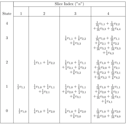
The recursion holds for every stateB at sliceN. There is no probability which depends uponB in equation (13), whereas the expression in Equation (6) explicitly incorporates the terminal state,B, and the frequency param-eters also depend uponB. In the case of equi-probable state transitions in the lattice, equation (13) specifies for every state a simple average of the values from the prior slice’s connected states.
2.3 Example of Forward Induced SCEV Values
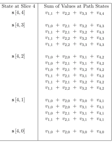
Table (1) illustrates how (13) successively forms expected values. For the game posed above, say the payoff occurs if and only if the path terminates in s[4,3]. The elements of the path spaces of slice N are given in Table (2). For s[4,3], e.g., v(1,1) occurs in three paths, and v2,1 occurs in two.
Accordingly, the coefficients onv1,1 andv2,1 are 3/16 and 1/8, respectively,
as indicated in Table (1).
2.4 SCEV Induction for More General Functionals.
Equation (13), as written, encompasses only the special case of the sum of the state variable values, since it embodies that specific elementary definition in equation (8). It can be generalized to embrace the definition of any linear combination of values which depend on the state variable’s values. Denote such a linear combination of state variable values along a path from the origin to s[N, B] by Λk(N, B), and denote the coefficient to be applied to of the n-th state value by λn. A simple example of such a functional is the discrete average of a stock’s price, taken every three months for five years, defined on a lattice with one month steps. For this example, Λ would be specified as: Λ1(N) = N=20 X n=1 λnv(i, bn) (14) λn = 1 20 , n={3, 6, . . . , 60}; λn = 0, otherwise. (15)
Table 1: Accumulation of Node Values in Forward Path Sums. Slice Index (”n”) State 1 2 3 4 4 161 v1,1+161v2,2 +161v3,3+161v4,4 3 18v1,1+18v2,2 161 v1,0+163v1,1 +18v3,3 +18v2,1+18v2,2 +163v3,2+161v3,3 +14v4,3 2 14v1,1+14v2,2 18v1,0+14v1,1 163v1,0+163 v1,1 +14v2,1+18v2,2 +161v2,0+14v2,1 +38v3,2 +161v2,2+163v3,1 +163v3,2+38v4,2 1 12v1,1 14v1,0+14v1,1 14v1,0+18v1,1 163v1,0+161 v1,1 +12v2,1 +18v2,0+14v2,1 +18v2,0+18v2,1 +38v3,1 +161v3,0+163v3,1 +14v4,1 0 12v1,0 14v1,0+14v2,0 18v1,0+18v2,0 161v1,0+161 v2,0 +18v3,0 +161v3,0+161v4,0
The corresponding SCEV values for slice N can be induced by the method implied in Equation (13). Denote the SCEV measure of the functional Λ1
by Φ. Then, Φ(Λ1(N) ;B) = 1 2 {Φ(Λ1(N −1) ;B) + Φ(Λ1(N−1) ;B−1)} + 1 2 {γ(N−1, B) +γ(N−1, B)}λN vN,B (16) The state variable is formally added at every slice, butλn is non-zero in this example only when n evenly divides by three; i.e., at the slices corre-sponding to the points of averaging.
Table 2: Path Sums to Slice 4
State at Slice 4 Sum of Values at Path States s[4,4] v1,1 + v2,2 + v3,3 + v4,4 s[4,3] v1,0 + v2,1 + v3,2 + v4,3 v1,1 + v2,1 + v3,2 + v4,3 v1,1 + v2,2 + v3,2 + v4,3 v1,1 + v2,2 + v3,3 + v4,3 s[4,2] v1,0 + v2,0 + v3,1 + v4,2 v1,0 + v2,1 + v3,1 + v4,2 v1,0 + v2,1 + v3,2 + v4,2 v1,1 + v2,1 + v3,1 + v4,2 v1,1 + v2,1 + v3,2 + v4,2 v1,1 + v2,2 + v3,2 + v4,2 s[4,1] v1,0 + v2,0 + v3,0 + v4,1 v1,0 + v2,0 + v3,1 + v4,1 v1,0 + v2,1 + v3,1 + v4,1 v1,1 + v2,1 + v3,1 + v4,1 s[4,0] v1,0 + v2,0 + v3,0 + v4,0
SCEV induction attains for multiplicative path functionals as well. In that case, the recursive specification for the functional has a different form; it does not entail the second term. It is easy to understand why this must be so. In a multiplicative functional, there is, for all n, only one term, formed successively by a single multiplication. The average of prior state values still provides the path-weighted expected content of the product prior to a slice, and the content of the term at the slice-state is formed by the same multiplication.
As an example, denote a path-wise product of state variable values along a path from the origin tos[N, B] by Ψ(N, B). Denote the term multiplied at a slicenasψn. The specification of a quarterly-averaged geometric Asian option, on a month-step-size lattice entails the functional:
Ψ(N) = N=20 Y n=1 ψn ψn(bn) = v(n, bn) 1 N, n={3,6, . . . ,60}; ψn(bn) = 1, otherwise. The SCEV measure of this is:
Φ(Ψ(N); B) = 1
2{Φ(Ψ(N −1); B)
+ Φ(Ψ(N −1); B−1)} ψN(B) (17)
2.5 Generalization for Moments.
SCEV values generally do not directly proscribe the value of a security or a cash flow. For example, while equation (16) provides information on the expected value of the quarterly average of stock prices, that does not itself provide the value of an Asian option. However, the expected Asian option payoff depends on the expiry-date probability distribution of the average. The first moment alone is not sufficient to identify an approximation to this distribution from which the value an Asian option could be inferred. But by applying at least a partial solution to the Problem of Moments (see Appendix A, and Section 4), a proxy to that distribution cast in terms of a sequence of successive moments will suffice in quite general circumstances. Since the m-th moment about zero is the expectation of the m-th power of the variate, each such expectation can be generated by SCEV induction applied with appropriate generalization.
Denote the functional of the arithmetic path average as in (14), now sub-scripted to indicate the first moment. Denote the square of that functional as Λ2. That is:
Λ2(N) = (Λ1(N))2 (18)
In light of the recursion of Λ1(N), and expanding the power, Λ2(N) takes
a form that entails terms of both the fundamental additive, as well as the multiplicative, forms:
Λ2(N) = { Λ1(N−1) + λnv(i, bn)}2
= (Λ1(N −1))2 + 2 Λ1(N−1)λnv(i, bn) + λn2v(i, bn)2 = Λ2(N −1) + 2 Λ1(N −1)λnv(i, bn) + λn2v(i, bn)2 Accordingly, the SCEV induction of Λ2(N), the second moment of the
arithmetic average, is:
Φ(Λ2(N);B) = 1 2 {Φ(Λ2(N−1);B) + Φ(Λ2(N−1);B−1)} + (2) 1 2 {Φ(Λ1(N −1);B) + Φ(Λ1(N −1);B−1)} λNv(N, B) + 1 2 {γ(N −1, B) +γ(N −1, B)}λN 2v(N, B)2 (19)
The SCEV induction of thek-th moment is generated analogously from the binomial expansion of Λ2(N) ={Λ1(N−1) + λnv(i, bn)}k.
2.6 The SCEV operator and conditional expectation.
At s[N, B], for an arbitrary path functional X(N), the SCEV operator Φ(X(N); B) is related to the conditional expectation of the functional by the probability density ofs[N, B]: γ(N, B). That is,
E(X(N) |vN,B) =
Φ(X; bN =B)
γ(N, B) (20)
It is an elementary result that the (unconditional) expected value of one of two jointly distributed random variables is the expected value of the conditional expectations, conditioned by the probability density of the other variate. That is, denoting an arbitrary path functional by X(N), jointly distributed withv[N, B]:
E(X(N)) = N
X
b=0
E(X(N)|vN,b) Pr (vN,b) (21)
From equation (20), the summands in equation (21 are each Φ(X(N);b). Thus, the expectation of the distribution of the functional, at slice N, is provided directly by the sum, over all statesb, of the values of the respective
These simple relationships of course apply to option values as well. De-note the m-th SCEV expectation functional as Φm(N;B); i.e., Φ2(N;B)
shortens Φ(Λ2(N);B) in (19). Denote the sum over all states B on slice N
as: Υm(N) = N X b=0 Φm(N;b).
If C(Φ1(N;B),Φ2(N;B) . . . Φm(N;B)) denotes the value of a contingent claim, conditional onv[N, B], then the unconditional value of the contingent claim is: C(Υ1(N),Υ2(N) . . . Υm(N)) = N X b=0 C(Φ1(N;b),Φ2(N;b) . . . Φm(N;b))γ(N, b) (22)
In Section 4, the Υm(N) represent expiry date values of successive mo-ments of the arithmetic average, and the call valuation methodology,C(.) is a method which employs those moments to infer the value of Asian options. Then equation (22) establishes that it is therefore possible to apply C(.) state-by-state, thereby obtaining state conditional option value, and then, by summing as in equation (21), obtain the unconditional option value.
Prior to that endeavor, a simpler exercise will be undertaken to demon-strate the fundamental efficacy of the approach, and establish some of the methodology subsequently employed in valuations. In the next section, the moments of the average of the state variable’s lattice values, and their limit-ing values under continuous averaglimit-ing, will be directly computed by SCEV induction, demonstrating that the moments thus obtained are numerically identical to the values derived by analytic means.
3
An Example: Conditional Moment Values for
Averaged Lattice States, and of the
Discretely-Averaged Continuous Process.
Finding moments of an average of values is a natural choice for demonstrat-ing SCEV induction. Not only can the values be determined analytically for direct comparison, but, further, the exercise entails all of the formulations in the previous section.
When the SCEV roll-forward method is employed, the values of the moments of the ”average” functional of thelog-binomiallydistributed repli-cating values will be obtained exactly. With diminishing lattice step size,
as these distributions converge to the finite-dimensional distributions gen-erated by the underlying process, so too will the moments. By forming, and extrapolating from, sequences of values from successively more dense replicating lattices, then the method will empirically provide the moments of averages of the continuous underlying process, taken at discrete intervals, or, as a special case, continuously.
3.1 The Values of the Moments of the Average of a Lattice’s Slice-State Values.
Owing to analytic simplicity of the binomial distribution, it is straightfor-ward to write down expressions for the moments of the values arrayed in the states of any slice.
It was established above that the subsequent values of a unit-valued security under a Wiener process with instantaneous expected return and volatility parameters r and σ (both per-annum)), over a one year horizon, is replicated by a binomial lattice of N steps, with step-time difference of dt= 1/N, with values: νn,b = eθndt e(2 b−n)σ √ dt whereθ = r− ln(cosh(σ √ dt)) dt (23) and thus νn,b = erndt sech(σ √ dt)n e(2b−n)σ √ dt (24)
For purpose of comparison, the moments of the average of N path-wise values on a lattice so constructed can be obtained using the expressions advanced in [[2]], as are there cast for the discretely averaged continuous process, but employing the moments of the values on the first lattice slice that corresponds to an averaging period. If the time of the first averaging corresponds to the first lattice slice, then them−th moment, say,µm of the two ”n= 1” lattice slice values is directly:
µm = exp(r dt)m sech(σ √ dt) m emσ √ dt+e−mσ√dt 2 ! = er m dt sech(σ √ dt)m cosh(mσ √ dt) (25)
3.1.1 Numerical example
In applying SCEV induction no ex-ante knowledge of the moments’ values is required; those values are, for this example, the result of running the algorithm. Further, the resultant moments, both state-conditional and un-conditional, are each simply a species of a functional ”of interest” for the issue at hand. In other applications, different functionals would be of in-terest: for example, the average of rates in valuation of an indexed note, or the average remaining outstanding balance, as indicated by an exogenous prepayment model, on a mortgage pool undergoing rate-dependent prepay-ment. Such functionals would be handled using fundamental methods no different than those in this example.
Appendix B gives Microsoft Visual Basic code which works this exam-ple.2
The procedure’s steps can be enumerated as follows:
1. Establish the slice-state values for the binomial lattice, implementing Equation (24).
2. Perform iterative calculations at each slice, n = 1, . . . , N, and, for the states within each slice, b = 0, . . . , n. At each state, induce the moments’ values with calculations that generalize Equation (19). 3. After processing through slice N, the values for each moment,
condi-tional upon each state of that terminal slice, will have been identified. Each of these values is the exact value of the moment of the path-wise averages, over the population of all paths which terminate at that node, weighted by the probability that that node was attained. Ac-cordingly, implementing equation (21), the unconditional moment is the simple summation of those values.
3.2 Generating SCEV Values When Some Steps Do Not Contribute to the Functional: Extrapolating to the Mo-ments of the Average of the Continuous Underlying Pro-cess.
The moments obtained by SCEV induction relate to discrete log-binomial
replicating distributions, and not to the underlying process except asymp-2If that code is implemented as a Microsoft Excel macro, the values of the first four
moments of the path-wise average, determined by SCEV induction, will show in the ”Im-mediate” window of the Visual Basic Editor.
totically. Thus, even if the averaging frequency under consideration is non-continuous, the lattice algorithm would not directly return the values asso-ciated with discrete sampling of the continuous process. An example of how this is accomplished is undertaken next.
The goal now is to find the moments of the average of values of the
underlying, i.e., continuous process, taken uniformly, as before, 12 times over one year.
Just as before, ”benchmark” values can be determined analytically, using the successive moments of a log-normal distribution as would prevail under the continuous process after one month. The only difference in application of the implemented SCEV algorithm now is that the state variable’s value con-tributes to the functionals−the moments−on only a subset of the lattices’ slices. Specifically, if the lattice employed has (in this instance) N = 12 k steps, only those slices with indexn such thatn modk= 0 will contribute to the SCEV values. At such indexed slices, theλnof equation(14) will have valueλn= 1/12; otherwise, λn= 0.
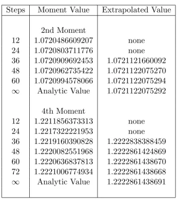
The rate of convergence of the replicating binomial distributions, and the associated moments, to the continuous value is not the same for all mo-ments. However, the assured certainty of, and regularity of, the convergence suggests that Richardson Extrapolation (”R.E.”) can be employed to good effect, with a varying number of lattice steps as the extrapolation’s domain. Table 3 shows the results of running the same algorithm employed in the first example, generalized to accommodate the differential slice-dependent ”weights,” with successively smaller lattice steps more closely replicating the one-year continuous evolution. Along with the second and fourth binomial moment value at each successive run, the R.E. estimates are provided in the table.
The rate of convergence in the extrapolates is far greater than in the successive lattice-values’ moments themselves. The extrapolation power is a result of the regularity and monotonicity of that convergence. Overall, the power of the extrapolation method applied to the moments is arguably quite remarkable. The convergence criterion was set to 10−12, and all the moments’ values were recovered to that accuracy, in, at most, 6 increments of 12 in lattice step count, from 12 to 72.
The use of moments as exemplary functionals to illustrate the effective-ness of SCEV induction was motivated in part by knowable benchmarks, but also to segue into the next section. There, the conditional moments, recov-ered by SCEV induction, have values that are not otherwise easily obtained, if at all. For each individual expiry state, those values will be employed to
ical integration of that proxy, subject to a particular payoff rule, produces state-conditional option values. Then, ultimately, those option values can be probability weighted, summed, and discounted to establish values for arithmetic averaged Asian options.
Table 3: Extrapolation to Continuous Moment Values with underlying moments σ= 20%, drift = 5%
Steps Moment Value Extrapolated Value 2nd Moment 12 1.0720486609207 none 24 1.0720803711776 none 36 1.0720909692453 1.0721121660092 48 1.0720962735422 1.0721122075270 60 1.0720994578066 1.0721122075294 ∞ Analytic Value 1.0721122075292 4th Moment 12 1.2211856373313 none 24 1.2217322221953 none 36 1.2219160390828 1.2222838388459 48 1.2220082551968 1.2222861424869 60 1.2220636837813 1.2222861438670 72 1.2221006774934 1.2222861438668 ∞ Analytic Value 1.2222861438691
4
Valuation of Arithmetic Asian options, With
both Fixed and Floating Strikes.
If the goal of of the lattice methods were simply establishing the moments of arithmetic averaging, then there are more efficient methods available. In this section, however, SCEV induction will be applied to a problem that has
no superior alternative, either in terms of computational effort, or, more importantly, in terms of efficacy. That problem is the valuation of floating strike Asian options.
Before turning the the floating strike case, however, the efficacy of using SCEV induction-derived conditional moments will be compared to alterna-tives in the widely studied and methodologically competitive case of fixed strike Asian options. There are a number of alternative methodologies for those valuations, of varying degrees of precision and computational effort. It is found that SCEV induction, along with quadrature using the moments, provides values at least as good as the best alternatives with superior com-putational cost.
4.1 Computational Strategy
For option valuation, the moments of the average recovered by SCEV in-duction are used to infer measures on the distribution of the average.
At least for moderate volatility levels, the Maximum Entropy (”ME”) method advanced by Fusai and Tagliani [[4]] is a demonstrably good empiri-cal approach to using moments to infer a proxy for the unknown distribution and, thereby, establish option values. Herein, a method is employed which is formally equivalent to an ME-determined distribution proxy for the dis-tribution of the averageitself, rather than a transform of that variate. The form of the proxy is described in Appendix A, where it is determined by an almost purely algebraic argument. As such, this proxy is simply referred to herein as the MM-proxy, denoting ”Moments-Method”, so to differentiate this proxy method from the more elegant and analytically extensible ME method advanced in [[4]]. There is, of course, no reason why such analyt-ically superior methods could not be used with SCEV induction on set of moments of an appropriately transformed functional of the average. As will be seen, at least for the range of option terms covered here, there is no reason to reach to the alternative ME framework.
The overarching result is that, in any case, there are advantages to employing the conditional moments. The main advantage accrues to the fact that any moment-based methodology, applied to the unconditional mo-ments, are powerless with regard to treating the joint distribution of stock price and average which is required for floating strike derivatives.
The SCEV induction approach is fundamentally structured to do pre-cisely that. The roll-forward ends with moments’ values conditional upon the state variable’s values at each ending state of the lattice slice corre-sponding to the expiry. In the examples before, these values were summed to obtain the unconditional moment values. An option value obtained with the MM method, applied at every slice-state of the expiry slice, using the conditional moments, is therefore also a value conditional upon the
termi-nal stock value. Together with the known probabilities on the states, those values can be summed, and discounted, to provide the unconditional fair option price. Moreover, that technique means that, with changes only in the specification of quadrature bounds −to entail the state’s stock level, rather than the fixed strike level−floating strike options can be valued in a framework no different than that used to value the fixed strike cases.
There is, as well, a modest advantage in numerical stability in the simple MM -proxy from using the conditional moments, for two reasons. Recall that the moments recovered by SCEV induction are over averages along only those paths in the path space of each ending state. Informally speaking, this tends to mitigate some of the collinearity found in the unconditional moments, which effects the numerical problems of proxy definition. Also, this mitigates the effects of higher volatility, which effect both numerical stability and convergence to distribution in increasing moment order.
The calculation strategy, for both fixed and floating strike options, can be summarized by these steps:
1. Recover the first2M moments for each state on sliceNi of a binomial
lattice (thus having time stepdti = 1/Ni year), with the index denoting
successively smaller step size.
2. Perform an MM-proxy valuation using order M on every state, with the payoff rule reflecting the the strike price being, as required, either fixed, or equal to the stock value at the state.
3. Sum the conditional option values thus determined (weighted by the prescribed slice-state binomial probabilities). That sum,ci, discounted
by the riskless rate, is an Asian option value, but in the context of a lattice of Ni steps, rather than the continuous underlying process.
Continue with step 1, decreasing step size until the Richardson method extrapolates a convergent limit with sufficiently small approximation error for the sequence ofci.
4.2 Comparative Results For Fixed Strike Options.
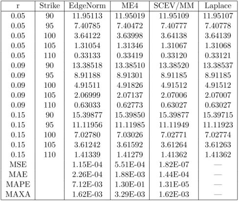
In [[4]], the authors report an excellent side-by-side comparison of results of most of the popular methods for Asian option valuation, applied across varying strike, drift, and volatility inputs. They, there, take as the ”bench-mark of true value” the values attained by numerical inversion of the Laplace transform of the Asian call advanced by Geman and Yor [[5]]. Along with the present results, obtained with the valuation strategy above, using an order 4
MM-proxy distribution, and the Laplace-transform based benchmark, com-parative values are reported for the two alternative methods which provided the best value estimates, on average, relative to that benchmark. These are an Edgeworth expansion around the normally distribution log of the average
−EdgeNorm−in the tables, and the order-four Maximum Entropy applied to the moments of the distribution of the log of the average. (See [[4]] for a detailed description of these methods).
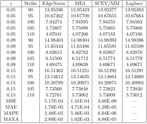
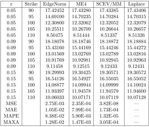
Relative to the analytic sophistication and need for numerical solution power surrounding the alternatives, SCEV/MM is very elementary indeed. Notwithstanding, its results dominate those of the others, and come very close to the benchmark itself. The results are found in Tables 4 through 6, for three different levels of volatility. SCEV/MM is superior to the alternatives on the basis of every norm: mean squared error (MSE), mean absolute error (MAE), mean absolute percentage error (MAPE), and maximum absolute error (MAXA).
Given this favorable comparison, it is worth noting that the SCEV/MM method can be extended to the case of discrete averaging, by the simple addition of the methodology employed in the second example of Section 2. There does not seem to be as meaningful a set of benchmarks to apply in these cases, and results are not reported. Further, in general, none of the alternative methodologies can strictly handle discrete averaging as a simple extension.
Moreover, as anticipated earlier, the method can be extended to floating strike options as well; again, this cannot be said for any of the alternatives. Application of SCEV/MM to floating strikes is undertaken next.
4.3 Valuation of Floating Strike Asian options.
There is a paucity of summarized valuations reported in the literature for Floating Strike options. However, Monte Carlo values reported with suffi-cient accuracy to constitute a meaningful valuation comparison are found in [[3]], and will be employed as a ”benchmark” for the floating strike values determined by the SCEV/MM method.
There are no changes to the SCEV/MM valuation strategy, except for the required changes to reflect the state-dependent strike price. The defini-tion of the payoff for the ”floating strike call” opdefini-tion is that to which the
Table 4: Comparison of SCEV/MM to Laplace Benchmark and Best Overall Published Alternative Methods
Annual Volatility Rateσ = 10%
r Strike EdgeNorm ME4 SCEV/MM Laplace
0.05 90 11.95113 11.95019 11.95109 11.95107 0.05 95 7.40785 7.40472 7.40777 7.40778 0.05 100 3.64122 3.63998 3.64138 3.64139 0.05 105 1.31054 1.31346 1.31067 1.31068 0.05 110 0.33133 0.33419 0.33120 0.33121 0.09 90 13.38518 13.38510 13.38520 13.38537 0.09 95 8.91188 8.91301 8.91185 8.91185 0.09 100 4.91511 4.91826 4.91512 4.91512 0.09 105 2.06999 2.07137 2.07006 2.07007 0.09 110 0.63033 0.62773 0.63027 0.63027 0.15 90 15.39877 15.39850 15.39877 15.39715 0.15 95 11.11956 11.11985 11.11949 11.11923 0.15 100 7.02780 7.03026 7.02771 7.02774 0.15 105 3.61242 3.61592 3.61264 3.61263 0.15 110 1.41339 1.41279 1.41362 1.41362
MSE 1.15E-04 5.51E-04 1.82E-07 —
MAE 2.26E-04 1.88E-03 1.44E-04 —
MAPE 7.12E-03 1.30E-01 1.31E-05 —
MAXA 1.62E-03 3.29E-03 1.62E-03 —
Monte Carlo results relate: a continuously averaged option whose payoff is, at European exercise in one year, any positive difference between the under-lying asset’s value at expiry and the average through expiry, i.e., a payoff c= max(S1−A1 , 0).
It arguably should not be anticipated a priori that the level of efficacy attained for fixed strike would necessarily propagate to the floating strike case. One reason for this is that there might be, informally speaking, some consistent ”averaging out” of discrepancies in the fixed strike cases as the algorithm progresses from one state to the next.
On the other hand, there is just as arguably no reason to assume that the fundamental efficacy of the method would be affected, since the only change is that of state-by-state variation of the strike level, and the method appears to maintain its accuracy across the range of strike prices. Ultimately, absent the kind of high-precision valuations as afforded in the fixed strike case, or,
Table 5: Comparison of SCEV/MM to Laplace Benchmark and Best Overall Published Alternative Methods
Annual Volatility Rateσ = 30%
r Strike EdgeNorm ME4 SCEV/MM Laplace
0.05 90 13.95336 13.95423 13.95377 13.95383 0.05 95 10.67462 10.67700 10.67655 10.67664 0.05 100 7.94274 7.94595 7.94555 7.94563 0.05 105 5.75607 5.75898 5.75865 5.75868 0.05 110 4.07041 4.07206 4.07183 4.07180 0.09 90 14.98403 14.98304 14.98393 14.98396 0.09 95 11.65443 11.65486 11.65581 11.65589 0.09 100 8.82615 8.82782 8.82867 8.82876 0.09 105 6.51500 6.51712 6.51774 6.51779 0.09 110 4.69475 4.69639 4.69671 4.69671 0.15 90 16.51362 16.51251 16.51292 16.51291 0.15 95 13.14612 13.14635 13.14664 13.14669 0.15 100 10.20789 10.20971 10.20975 10.20983 0.15 105 7.73560 7.73848 7.73823 7.73830 0.15 110 5.72761 5.73062 5.73009 5.73012
MSE 5.17E-04 1.41E-04 3.60E-09 —
MAE 1.78E-03 4.71E-04 5.29E-05 —
MAPE 2.48E-02 5.46E-03 6.04E-06 —
MAXA 2.89E-03 1.02E-03 8.88E-05 —
alternatively, advances to close, paired, bounds on floating strike values, or, as is most likely, even higher precision Monte Carlo values, the issue cannot be definitively resolved.
The Richardson Extrapolation again played an important role in deter-mining the estimated values. In every instance, the R.E. converged to three decimal places after processing a lattice of 256 steps. The lattices’ step count began with 64 steps in each case, and increased by 64 for each additional re-quired evaluation, with the convergence thus being attained after the fourth lattice evaluation.
Table 7 shows the results, both for the intermediate option values as returned from the lattice valuation, and the R.E. extrapolated values, for the case with σ = 0.10. It is clear that, without the R.E., much more
Table 6: Comparison of SCEV/MM to Laplace Benchmark and Best Overall Published Alternative Methods
Annual Volatility Rateσ = 50%
r Strike EdgeNorm ME4 SCEV/MM Laplace
0.05 90 17.42452 17.43280 17.43385 17.43406 0.05 95 14.69100 14.70235 14.70284 14.70315 0.05 100 12.30800 12.32062 12.32052 12.32079 0.05 105 10.25511 10.26709 10.26644 10.26657 0.05 110 8.50475 8.51444 8.51337 8.51326 0.09 90 18.18078 18.18746 18.18872 18.18884 0.09 95 15.43160 15.44169 15.44246 15.44272 0.09 100 13.01569 13.02769 13.02789 13.02816 0.09 105 10.91769 10.92981 10.92945 10.92963 0.09 110 9.11458 9.12515 9.12433 9.12431 0.15 90 19.29993 19.30425 19.30571 19.30572 0.15 95 16.54126 16.54927 16.55035 16.55052 0.15 100 14.08877 14.09944 14.09999 14.10024 0.15 105 11.93397 11.94578 11.94579 11.94600 0.15 110 10.06033 10.07171 10.07119 10.07128
MSE 2.75E-03 2.35E-04 3.82E-08 —
MAE 1.05E-02 7.99E-04 1.73E-04 —
MAPE 8.38E-02 5.90E-03 1.32E-05 —
MAXA 1.28E-02 1.47E-03 3.05E-04 —
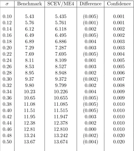
Notwithstanding the caveats above mentioned to extending SCEV/MM to floating strike cases, Table 8 indicates that the efficacy demonstrated for fixed strikes very likely does persist. In no case were the three decimal place SCEV/MM results different by more than possible rounding error in the two decimal place benchmarks. Because of the latter degree of precision in reporting, the reported confidence interval cannot be used directly, but in every case, save one, the SCEV/MM results round to exactly the same value as the corresponding benchmark.
It perhaps deserves mention that [[6]] considers the value of an ”in progress” floating strike option, i.e., one which is valued at some point in time after the start of averaging, conditional upon the value of the stock at that point. To this end, they provide an upper bound formulation, as well as high precision Monte Carlo values. The in-progress valuation could be readily be undertaken using SCEV/MM method, but it will not be done in
Table 7: Lattice and Extrapolated Values Steps Lattice Richardson Richardson
Value Extrapolation Confidence
64 5.3588 5.3588 none
128 5.3970 5.3970 none
196 5.4097 5.4353 .026
256 5.4160 5.4351 -.00008
this paper.
The next section discusses some of other asset classes for which path-dependent features can be analyzed with SCEV induction, particularly in cases where the operative functionals are a security’s cash flows.
5
Comments on Extensibility of SCEV Induction
to other Asset Classes.
There are a large number of financial claims modelled with more-or-less vanilla Wiener diffusion processes; some important classes being claims structured on the market levels of currencies and commodities. Many differ-ent kinds of path-dependdiffer-ent structures can be efficidiffer-ently valued using SCEV operators on the functionals defining the payoffs of these claims, many with-out fundamental change in specification or application from that advanced in this paper.
This section describes some overall implications, as well as discussion of asset classes which would require to the underlying generalization of the elementary developments of Section 2.
5.1 The Implication for Monte Carlo Methods.
Perhaps the most general implication for application of SCEV induction arises from the floating strike analysis above. That implication is far more general than the efficacy of valuation in that particular case. Rather, it is in regard to the way in which high-precision results can be obtained without the setup effort, transformational methodology, and computer time which attends Monte Carlo.
formula-Table 8: Floating Strike Asian Call Values, By Volatility with riskless rate constant at = 10%
σ Benchmark SCEV/ME4 Difference Confidence
0.10 5.43 5.435 (0.005) 0.001 0.12 5.76 5.761 (0.001) 0.001 0.14 6.12 6.118 0.002 0.002 0.16 6.49 6.495 (0.005) 0.002 0.18 6.89 6.886 0.004 0.003 0.20 7.29 7.287 0.003 0.003 0.22 7.69 7.695 (0.005) 0.004 0.24 8.11 8.109 0.001 0.005 0.26 8.53 8.527 0.003 0.005 0.28 8.95 8.948 0.002 0.006 0.30 9.37 9.372 (0.002) 0.007 0.32 9.80 9.799 0.002 0.008 0.34 10.23 10.226 0.004 0.009 0.36 10.65 10.655 (0.005) 0.009 0.38 11.08 11.085 (0.005) 0.010 0.40 11.51 11.515 (0.005) 0.010 0.42 11.95 11.947 0.003 0.010 0.44 12.38 12.378 0.002 0.010 0.46 12.81 12.810 0.000 0.010 0.48 13.24 13.242 (0.002) 0.020 0.50 13.67 13.674 (0.004) 0.020
implemented in replicating lattices, a SCEV induction can be designed to expose exactly the information that would attain from anexhaustiveMonte Carlo; that is, one which actually considered every path through the prob-ability space. The latter approach is effectively impossible, and, as such, SCEV will dominate the results of any path-sample based Monte Carlo, and do so with a vanishingly small proportion of the calculations required for a Monte Carlo for the same practical level of precision in result. This will attain even relative to Monte Carlo valuations cast in terms of a continuous process, so long as, once again, that process can be replicated by a sequence of successively more dense lattice models convergent in probability to the underlying process’ continuous distributions.
5.2 Extension to Lattice Models Which Preclude 50-50 Bi-nomial State Transitions.
There are stochastic models which will not accommodate lattice replication with 50-50 binomial branching. By definition, trinomial lattices do not, and in cases where certain interest rate processes can be replicated in bino-mial form, but the branching probabilities must be taken as an endogenous parameter to affect the replication.
SCEV induction can still be applied to such constructions, albeit with required generalization of the development in Section 2. The form and substance of such generalizations are for the most part straightforward and readily apparent, and have not been undertaken −nor required− for the Asian option examples in this paper.
5.3 Extensions to other asset types and structures.
Potentially, wide application can be found among debt securities and interest rate dependent derivatives. Structures with path dependent cash flows are abundant among debt securities. Some types of debt claims which lend themselves to SCEV induction on their cash flows include:
• Index Amortizing notes and swaps, where principal retirement is func-tionally related to rate levels, and possibly to elapsed term;
• Average interest rate caps and floors;
• Periodic and Ladder cap or floor structures;
• Optional multiple sinking fund operations;
• Mortgage backed securities, or, more generally, securities which embed multiple holder− or issuer− options which collectively induce partial principal retirement.
MBS securities present some of the most challenging valuation problems in finance. Accordingly, further discussion is warranted regarding the role which SCEV induction might play in their analysis.
5.4 Mortgage backed securities issues.
The arbiter of feasibility of implementing SCEV induction in MBS valua-tion is the nature of the prepayment model (”PM”) employed. Prepayment
mortgages at the time of analysis: Weighted Average Maturity, Weighted Average Coupon, Loan-to-Value ratio, and so on. Moreover, the PM will generally specify at least three elements which are functionally dependent on the stochastically evolving refinance level to specify the intensity of ex-ercise of the refinancing option by the holders of the mortgages in the pool. Beyond the rate level incentive itself, these generally entail some rate-based proxy for ”burnout”, such as a count of visitations to a profitable refinance rate without having complete refinancing within the pool, and also some measure of the term structure’s forward slope, which may proxy incentive levels.
To the extent that the prepayment rate is a function of those variables, then application of SCEV induction to path-wise sequences of prepayment rates, through lattice replications of the underlying rate term structure, is feasible. A lattice node’s prepayment rate, coupled with the expected remaining pool at the node, can in that case directly determine that node’s expected principal cash flows.
However, a PM will often include determinants which are not functions of the refinance rate or of the evolving ”conditions” of a pool. One such determinant is housing value, modelled in future states as being either in-dependent of, or imperfectly correlated with, the state’s rate environment. Housing value relates to mortgage default rates (the holder’s ”put” option on the mortgage), as well as, if principal recovery is not guaranteed to the MBS holder, the expected recovery upon foreclosure. These cannot be di-rectly modelled by SCEV induction.
In general, for SCEV induction to play any role in prepayment valuation, it is required that the PM be of an ”econometric” design. That is, the PM should be structured so that the modelled prepayment rate is attained by applying prevailing (or average) future levels of the input variables to an essentially linear system of equations.
A good example of a freely available, fully specified prepayment model is the one which has been estimated for, and maintained by, the Office of Federal Housing Enterprise Oversight (”OFHEO”), as an essential com-ponent of their Risk-based Capital Rules [[8]], and programmed into the software implementation of the Risk-based Capital Simulation Application. This model’s domains of variation entail all of the elements described above, both those which can be handled in an implementation employing SCEV in-duction, and those which cannot.
Conclusively, SCEV induction offers clear promise, but certainly not panacea, for lattice implementations completely precluding Monte Carlo, or other methods, in efficient valuation of mortgage backed securities.
References
[1] A. Abrahamson, A Note on Constructing 50-50 Step Probability Bino-mial Lattices to Replicate Wiener Diffusion,EconWPA Working Paper
(2003) pdf:
http://econwpa.wustl.edu:8089/eps/fin/papers/0305/0305004.pdf [2] A. Abrahamson, All Moments of Discrete and Continuous Arithmetic
Averages on Brownian Paths: A Closed Form,EconWPA Working Pa-per (2002) pdf:
http://econwpa.wustl.edu:8089/eps/fin/papers/0205/0205004.pdf [3] S. Chung, M. Shackleton, R. Wojakowski, Quadratic efficient
approx-imation of floating strike Asian option values, Sciences Economiques Sociales et de Gestion Working Paper (2000) pdf:
http://www.eco.fundp.ac.be/affi2001/I10.pdf
[4] G. Fusai and A. Tagliani, An Accurate Valuation of Asian Options Us-ing Moments,International Journal of Theoretical and Applied Finance
5(2) (2002) 147-169.
[5] H. Geman and M. Yor, Bessel processes, Asian options and perpetuities,
Mathematical Finance 3(4) (1993) 349−375.
[6] V. Henderson, D. Hobson, W. Shaw, and R. Wojakowski, Bounds for Floating-Strike Asian Options using Symmetry, Oxford University Mathematical Finance Paper(2003) pdf:
http://www.finance.ox.ac.uk/pages mfpapers/2003mf04.htm.
[7] M. Kendall, and A. Stuart,The Advanced Theory of Statistics, Volume 1. New York:Hafner Publishing Company, 1969.
[8] Office of Federal Housing Enterprise Oversight, Risk Based Capital Reg-ulation Amended Final Rule (As of February 12, 2003), 12 CFR Part 1750, 2003.
[9] J. Shohat and J. Tamarkin, The Problem of Moments, Providence, RI: American Mathamatical Society, 1963.
APPENDICES
A
A Simple Method-of-Moments Based
Distribu-tion Proxy.
In 1895 Stieltjes published a classical paper, ”Recherches sur les fractions continues”, which first formally posed what he termed the ”Problem of Moments.” The issue is to identify a function,ψ(x), such that, for prescribed valuesµ1, µ2, . . .,
µn=
Z ∞
0
xn ψ(x)dx (A-1)
He completely solved the issue of conditions of determinacy of such a function, and the Problem has come to formalize some fundamental concerns of characterization in mathematical statistics. A definitive text devoted entirely to the issues of characterizing distributions by their moments, and of existence of representations, is that of Shohat and Tamarkin [[9]].
If one can identify a solution to the moment problem, then that function might share other distributional characteristics in common with the distri-bution, perhaps unknown, which has the prescribed moments. In particular, iff(x) denotes that distribution function, and assuming that f(x)6=ψ(x), then one could employ the latter to proxy the former in questions of distri-bution. Specifically, the two quadratures:
P r(x < X) = Z X 0 f(x)dx≈ Z X 0 ψ(x)dx and v(x) = Z X 0 x f(x)dx≈ Z X 0 x ψ(x)dx are of central importance in numerical option valuation.
While [[9]] devotes not even a single page directly to issues of construction
−i.e., of actually finding a form for ψ(x)− it is easy to identify a feasible and computationally efficient form. This is particularly true if one adopts the position taken by Kendall and Stuart [[7]] in their discussion of the often divergent and generally unstable properties of Edgeworth series and its equivalent predecessor, the Gram-Charlier Type A series:
”From the statistical viewpoint, however, the important question is not whether an
infiniteseries can represent a frequency function, but whether a finite number of terms can do so to a satisfactory approximation.” (at Section 6.23).
A natural candidate for ψ(x) is clearly suggested by the nature of the problem: the problem entails a system of equations of the form in equation (A-1), and that implies the necessity of expressing each moment linearly in terms of others. Among simple functions, most elementary one that can generate such ”moment” expressions is:
ψ(x) =e−pM(a;x), (A-2)
wherepM(a;x) is a polynomial in x, of order M:
pM(a;x) =a0+a1x+a2x2+· · ·+aMxM such that e−pM(a;0) ≈ 0 and lim x→xH e−pM(a;x) ≈ 0
for some relatively large (strictly, infinite) value xH, and is otherwise uni-modal and strictly positive forx≤xH.
An algebraic solution can be written down if there exists a set of M+ 1 constantsam such that, for the first 2M moments,
µm=
Z ∞
0
xm e−pM(a;x)dx.
By re-writing the integral in each of the first M equivalences using in-tegration by parts, M equations in the M unknowns are defined, which entail the first 2M moments. For example, for the equivalence to the fourth moment, substituting equation (A-2) into (A-1):
µ4 = Z ∞ 0 x4 e−pM(a;x)dx ≡ − Z ∞ 0 x5 5 d dxpM e −pM(a;x)dx 5µ4 = Z ∞ 0 a1 x5+ 2a2x6+ 3a3x7+ 4a4x8+. . . e−pM(a;x) 5µ4 = a1 µ5+ 2a2 µ6+ 3a3 µ7+ 4a4 µ8+. . .
The coefficients for the distribution proxies employed in the empirical investigations in this article are solutions to the 4 x 4 system for particular
prescribed moment values: 2µ1 3µ2 4µ3 5µ4 = µ2 2µ3 3µ4 4µ5 µ3 2µ4 3µ5 4µ6 µ4 2µ5 3µ6 4µ7 µ5 2µ6 3µ7 4µ8 a1 a2 a3 a4
Solution of this system is generally numerically unstable for the moment values encountered for the averages; the determinant of the matrix is very close to nil. The solutions, however problematic, nonetheless work well empirically. The constant a0 does not enter the system. Its value that is
that which satisfies the condition of unit area undere−pM(a;x).
For the implementing computer programs, solution equations for each am, entailing the input moments, were pre-determined analytically. This obviated the need for matrix inversion, and, more importantly, permitted the numerical solutions to be carried out with extended precision arithmetic; in this case, 32 decimal-place significance was employed, using the public-domain MAPM arbitrary-precision math library. Once the polynomial co-efficients of first and higher order were determined, subsequent required nu-merical integrations could be carried out with conventional double-precision hardware arithmetic.
It is important to recognize that this form has not been demonstrated to be a solution to Stieltjes’ Problem, and in present application is not. An identical form, developed by other means, has a central position in the Maximum Entropy method (see [[4]]). That work considers the the issue of determinacy of solutions to the Problem of Moments for the distributions of the arithmetic average. Their conclusions, along with the numerical issues, there lead the authors to consider the distribution of a transform of the averages.
Because the development here has only the goal of generating a distri-bution proxy for empirical application, and because the Maximum Entropy method is advanced in the Asian option literature in much more formal, alternative, development, a more generic terminology −Moments-Method proxy, or simply ”MM”−is adopted to refer to the use of the form to infer the required measures on the unknown distribution.
A.1 An Example of an MM Proxy Distribution.
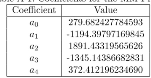
This example shows the MM proxy of the path-wise lattice-value averages for a particular case, viz., that of the state ”two sigma” below the mean on the 64-step lattice replicating values of a unit-based stock price over one
year, with a drift rate of 5% andσ of 30%. The state variable’s value there is about 0.55. The coefficients are:
Table A-1: Coefficients for the MM Proxy
Coefficient Value a0 279.682427784593 a1 -1194.39797169845 a2 1891.43319565626 a3 -1345.14386682831 a4 372.412196234690
The magnitude of the coefficients’ values indicates why extended precision arithmetic is needed in solution: the sizes of the values, and even more to the point, the disparities in order of different terms in the solution equations, in general are so great that loss of significance will destroy the efficacy of the resultant proxy if only conventional 16-place hardware floating point arithmetic is used.
Figure 1 shows the resultant density function of the MM proxy which employs these coefficients. That function is:
ψmm(x) = exp(−
4
X
0
aixi),
with the coefficients shown in Table A-1.
The function at least appears to be a well formed distribution, does pos-sess unit area and has the first eight moments match the values determined by the SCEV induction, and, most importantly, as the empirical results would attest, performs well as a proxy for the actual, unknown, distribution. Some insights into how well the proxy might match the actual distribution are available in the statistics literature (see, again, [[4]] for references and discussion.) To highlight the power and importance of these methods, if somewhat serendipitously, it may be pointed out that it would be possible to discover ”how close” the proxy is to the actual distribution in this case to full computational precision. One could evaluate the average of the val-ues along every path through the lattice to the referenced state. There are 250,649,105,469,666,120 such paths. However, since even at a rate of one million paths per second, the analysis would take a few less than 8,000 years, it was not undertaken for this Appendix.
APPENDICES
B
Visual Basic Code Implementing SCEV
Induc-tion Example of SecInduc-tion 3.1.
The following code implements SCEV induction to obtain the first few mo-ments of the pathwise averages of a lattice’s values. It is intended to be run as aMicrosoft Excelmacro, and then, in the Visual Basic editor. The Editor is accessed from Excel via ToolsMacro. AfterInsert of a new Module, the code can be copied verbatim. With the cursor in subroutine runMeAsEntry-Point(), F5 will produce the average moment’s values in the ”Immediate” window of the editor. Alternatively, F8 will begin a line-by-line step-through of the code, whereupon variable’s values can be seen by placing the cursor on a variable in the code.
A cut-and-paste of extracted text is the most efficient way to implement this code. A reader lacking a commercial desktop tool for that purpose can employ the Ghostscript/GSview package, which offers text extraction from PDF files.
To validate the application, the analytic values of the moments of the path-wise average of the log-binomial state values, say, ζα(m), m = 1. . .4, for the lattice implementing parameters r = 0.05, σ = 0.20, N = 12, are given here to one more decimal place of precision than provided by the code’s results:
ζα(1) = 1.027559706741054 ζα(2) = 1.072048660920718 ζα(3) = 1.135578546030313 ζα(4) = 1.221185637331294
Option Explicit
Public Const cBinProb = 0, cValue = 1, cMoments = 2 Dim retV As Variant
Private Sub runMeAsEntryPoint() getStateAverageMoments _
maxMoments:=4, stepsInYear:=12, sigma:=0.2, rate:=0.05 End Sub
Public Function fitLogNormal( _ Vals As Variant, _
Nmax As Integer, dt As Double, sig As Double, r As Double _ ) As Boolean
Dim n As Integer, b As Integer, bpLast As Double, exp_tdt As Double, _ exp_tndt As Double, ssR As Variant, theta As Double, arg As Double
ReDim Vals(0 To Nmax)
For n = 0 To Nmax: ReDim vSlice(0 To n): Vals(n) = vSlice: Next n ReDim vFacts(cBinProb To cMoments): Vals(0)(0) = vFacts
Vals(0)(0)(cBinProb) = 1#: Vals(0)(0)(cValue) = 1# ReDim crrStateVals(-Nmax To Nmax): crrStateVals(0) = 1#
arg = Exp(sig * Sqr(dt)): theta = r - Log(0.5 * (arg + 1 / arg)) / dt exp_tdt = Exp(theta * dt): exp_tndt = exp_tdt
For n = 1 To Nmax
crrStateVals(n) = crrStateVals(n - 1) * arg crrStateVals(-n) = 1 / crrStateVals(n) bpLast = 0
For b = 0 To n - 1 Vals(n)(b) = vFacts
Vals(n)(b)(cBinProb) = bpLast
bpLast = Vals(n - 1)(b)(cBinProb) * 0.5
Vals(n)(b)(cBinProb) = Vals(n)(b)(cBinProb) + bpLast Next b
Vals(n)(n) = vFacts: Vals(n)(n)(cBinProb) = bpLast For b = 0 To n
Vals(n)(b)(cValue) = exp_tndt * crrStateVals(2 * b - n) Next b
exp_tndt = exp_tndt * exp_tdt Next n
fitLogNormal = True End Function
Public Sub getStateAverageMoments(maxMoments As Integer, _ stepsInYear As Integer, sigma As Double, rate As Double)
Dim ssVals As Variant, n As Integer, b As Integer, dt As Double, _ m As Integer, lastSlice As Integer, momSet As Variant
dt = 1 / CDbl(stepsInYear): lastSlice = stepsInYear retV = fitLogNormal(ssVals, stepsInYear, dt, sigma, rate) ReDim momSet(0 To maxMoments), vUncondMoments(1 To maxMoments) For m = 1 To maxMoments: momSet(m) = 0: Next m
ssVals(0)(0)(cMoments) = momSet For n = 1 To lastSlice
For b = 0 To n
retV = SCEVaverageMoments(ssVals, n, b, maxMoments, _ ssVals(n)(b)(cValue) / stepsInYear) If (n = lastSlice) Then
vUncondMoments(m) _ = vUncondMoments(m) + ssVals(n)(b)(cMoments)(m) Next m End If Next b Next n For m = 1 To maxMoments
Debug.Print "Avg. Moment " & m, vUncondMoments(m) Next m
End Sub
Public Function SCEVaverageMoments( _ ssVals As Variant, _
n As Integer, b As Integer, MomMax As Integer, argVal As Variant _ ) As Boolean
Dim m As Integer, mm As Integer, fwdAvg As Variant, ssMoms As Variant, _ upM As Double, dnM As Double, combM As Double, _
valAvg As Double, valPwr As Double, sumMs As Double
ReDim ssMoms(1 To MomMax): For m = 1 To MomMax: ssMoms(m) = 0: Next m ReDim fwdAvg(1 To MomMax)
For m = 1 To MomMax fwdAvg(m) = 0 If (b < n) Then _
fwdAvg(m) = fwdAvg(m) + 0.5 * ssVals(n - 1)(b)(cMoments)(m) If (0 < b) Then _
fwdAvg(m) = fwdAvg(m) + 0.5 * ssVals(n - 1)(b - 1)(cMoments)(m) upM = 0: combM = 1: dnM = m
valPwr = argVal sumMs = 0
For mm = m - 1 To 1 Step -1
upM = upM + 1: combM = (combM * dnM) / upM: dnM = dnM - 1 sumMs = sumMs + combM * valPwr * fwdAvg(mm)
valPwr = valPwr * argVal Next mm
ssMoms(m) = fwdAvg(m) + sumMs + ssVals(n)(b)(cBinProb) * valPwr Next m
ssVals(n)(b)(cMoments) = ssMoms: SCEVaverageMoments = True End Function