Robust LQR Controller Design for Stabilizing and Trajectory Tracking of Inverted Pendulum

Procedia Engineering 64 ( 2013 ) 169 – 178

1877-7058 © 2013 The Authors. Published by Elsevier Ltd. Open access under CC BY-NC-ND license. Selection and peer-review under responsibility of the organizing and review committee of IConDM 2013 doi: 10.1016/j.proeng.2013.09.088

ScienceDirect

International Conference On DESIGN AND MANUFACTURING, IConDM 2013

Robust LQR Controller Design for Stabilizing and Trajectory

Tracking of Inverted Pendulum

Vinodh Kumar E

*, Jovitha Jerome

a_{Research Scholar, Department of Instrumentation and Control Systems Engineering, PSG College of Technology, Coimbatore, India-641004.} b_{Professor, Department of Instrumentation and Control Systems Engineering, PSG College of Technology, Coimbatore, India-641004.}

Abstract

This paper describes the method for stabilizing and trajectory tracking of Self Erecting Single Inverted Pendulum (SESIP) using Linear Quadratic Regulator (LQR). A robust LQR is proposed in this paper not only to stabilize the pendulum in upright position but also to make the cart system to track the given reference signal even in the presence of disturbance. The control scheme of pendulum system consists of two controllers such as swing up controller and stabilizing controller. The main focus of this work is on the design of stabilizing controller which can accommodate the disturbance present in the system in the form of wind force. An optimal LQR controller with well tuned weighting matrices is implemented to stabilize the pendulum in the vertical position. The steady state and dynamic characteristics of the proposed controller are investigated by conducting experiments on benchmark linear inverted pendulum system. Experimental results prove that the proposed LQR controller can guarantee the inverted pendulum a faster and smoother stabilizing process with less oscillation and better robustness than a Full State Feedback (FSF) controller by pole placement approach.

© 2013 The Authors. Published by Elsevier Ltd.

Selection and peer-review under responsibility of the organizing and review committee of IConDM 2013.

Keywords: Inverted Pendulum, LQR Controller, PV Controller, Riccatti Equation, Full State Feedback Controller, Pole placement approach 1.Introduction

Inverted pendulum is an unstable, nonlinear, multivariable, fourth order, and under actuated system which can be treated as a typical control problem to study various modern control theories. The control of inverted pendulum

* Corresponding author. Tel.: +91-9962093935; E-mail address:[email protected]

© 2013 The Authors. Published by Elsevier Ltd. Open access under CC BY-NC-ND license.

resembles the control systems that exist in some of the real time applications such as rockets and missiles, heavy crane lifting containers and self balancing robots. According to control purposes of inverted pendulum, the control of inverted pendulum can be divided into three aspects. The first aspect that is widely researched is the swing-up control of inverted pendulum [1, 2]. The second aspect is the stabilization of the inverted pendulum [3-4]. The third aspect is tracking control of the inverted pendulum [5]. In practice, stabilization and tracking control is more useful for plenty of real time applications. There are several problems to be solved in the control of inverted pendulum, such as swinging up and catching the pendulum from its stable pending position to the upright unstable position, and then balancing the pendulum at the upright position during disturbances, and further move the cart to a specified position on the rail [6]. Several methods for achieving swing-up and stabilization of pendulum system have been proposed in literature. In [7], a conservative law is derived from Lyapunov functions having a certain zone of non-convergence. A basic method of swing up control using energy methods for a cart-less pendulum has been proposed in [8]. This method has an advantage of a hierarchical nature, first controlling the pendulum angle, then the hinge position. However, in practical setups, there is an inherent limitation on the cart length and the magnitude of control force that can be applied. This gives the motivation to find out energy based methods for controlling and stabilizing the cart position with restricted cart length and restricted control force. The goal of this contribution is to implement the target tracking and stabilizing controller in real time for the linear inverted pendulum based on the control concepts of LQR theory and to report the disturbance rejection property of the LQR controller.

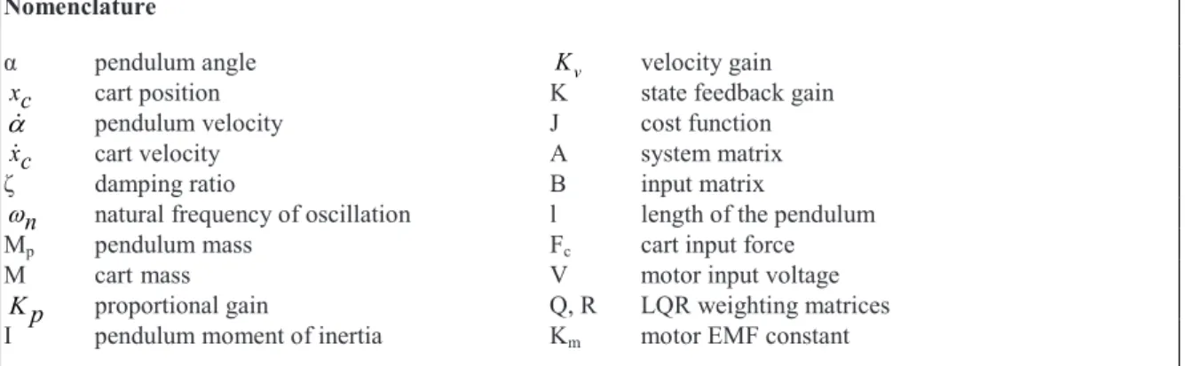
Nomenclature

pendulum angle K_v velocity gain

xc cart position K state feedback gain

pendulum velocity J cost function

xc cart velocity A system matrix

damping ratio B input matrix

n natural frequency of oscillation l length of the pendulum

Mp pendulum mass Fc cart input force

M cartmass

K p proportional gain Q, R LQR weighting matrices

I pendulum moment of inertia Km motor EMF constant

2.System Model

The linear Self Erecting Single Inverted Pendulum (SESIP) consists of a pendulum system which is attached to a cart equipped with a motor that drives it along a horizontal track. The schematic diagram of inverted pendulum system is shown in Fig. 1. The motor attached to the cart is used to adjust the position and velocity of the cart and the track restricts the cart movement in the horizontal direction. Encoders are attached to the cart and the pivot in order to measure the cart position and pendulum joint angle, respectively.

2.1 Single Inverted Pendulum Equation of Motion

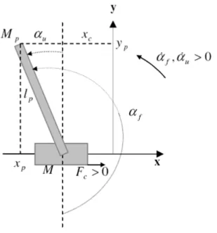
The schematic diagram and angle definitions of SESIP are shown in Fig. 2. The single inverted pendulum (SIP) system is made of a motor cart on top of which pendulum is pivoted. The movement of the cart is constrained only in the horizontal x direction, whereas the pendulum can rotate in the x-y plane [9]. The SIP system has two DOF

and can be fully represented using two generalized coordinates such as horizontal displacement of the cart, _xc and

rotational displacement of pendulum, negligible.

Fig. 2. SESIP Schematic

Applying Euler-Lagrangian energy equation to SESIP schematic shown in Fig. 2 results in

d L L

Qxc

dt x_c x_c (1)

and d L L Q

dt (2)

With L T_T V_T where T_T is total kinetic energy, V_T is total potential energy, _Qxc and Q are the generalized

force applied on the coordinate

x

( ) (t) B

Q_xc t F_{c eq c}x (3)

and Q B_p (t) (4)

This energy is usually caused by its vertical movement from normality (gravitational potential energy) or by a spring related sort of displacement. The cart linear motion is horizontal and as such, never has vertical displacement. So the total potential energy is full

characterized below:

cos( (t))

V_T M gl_{p p} (5)

The amount of energy in a system due to its motion is measured by the kinetic energy. Hence, the total kinetic energy can be depicted as follows:

T T T c p

T (6)

Where _Tc and _Tp are the sum of the translational and rotational kinetic energies arising from both the cart and its

mounted inverted pendulum, respectively. First, the translational kinetic energy of the motorized cart _Tct , is

expressed as follows:

2

1 2

T_ct Mx_c (7)

or, _Tcr , can be represented by:

2 2 1 2 2 J K_{m g c}x Tcr _rmp (8)

ten as shown below:

2

1 2 c cx

T_c M (9)

Where M_c M (J K / r_{m g mp}2 2 )

The total kinetic energy of the pendulum, T_p ,is the sum of translational kinetic energy, T_pt and rotational kinetic

energy, T_pr . 1 2 1 2 (t) 2 2 T T M r I p pt pr p p p T (10)

Where r_p2 x_p2 y2_p. From Fig. 2

x

y

cos( (t)) (t)

p c p

x x l (11)

and y_p l_psin( (t)) (t) (12)

Substituting (9), (10),(11),(12) into (6), gives the total kinetic energy,

T

2 2 2

1

1

(M

M ) ( ) M

cos( (t)) (t) (t)

(I

M I )

(t)

2

2

T

x t

l

x

The Lagrangian can be expressed using (5) and (13)

2 2 2 _{cos( (t))}

1

1

(M

M ) ( ) M

cos( (t)) (t) (t)

(I

M I )

(t)

2

2

T

x t

l

x

From equation (1) and (2), the non linear equation of motion can be obtained as: 2

(M M ) ( ) B

x t

x

(t) (M

l

cos( (t)) (t)

M l

sin( (t)) (t)

F

(t)

and

M

l

cos( (t)) ( ) (I

x t

M

l

) (t) B

(t) M g sin( (t)) 0

l

The nonlinear model can be linearized around the equilibrium point (upright pendulum) so thatsin( ) ,cos( ) 1. The design of state feedback controller requires the mathematical model of the system in state space form. Thus the linearized model of inverted pendulum in state space form can be written as

X AX BU (17)

Y CX

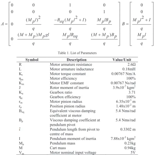
0 0 1 0 0 0 0 1 2 2 ( ) 0 ( ) ( ) 0 M lB ) ( ) )2 ( 2 p ))))) eq((((( p )) M lBp p A q q q M M_p))))M glM gl_pg M lBM lB_{p eq} (((((MM MM_p))BB_p q q q 0 0 2 M l_p 2 I B q M l_p q

Table 1. List of Parameters

Symbol Description Value/Unit

R Motor armature resistance

L Motor armature inductance 0.18mH

Kt K

K Motor torque constant 0.00767 Nm/A

m Motor efficiency 100%

Km Motor EMF constant 0.00767 Ns/rad J Rotor moment of inertia 3.9x10-7_kgm2

Kg Gearbox ratio 3.71

g Gearbox efficiency 100%

rm Motor pinion radius 6.35x10-3m rp

r Position pinion radius 1.48x10-2_m Beq Equivalent viscous damping

coefficient at motor

5.4 Nms/rad Bp Viscous damping coefficient at

pendulum pivot 5.4 Nms/rad Pendulum length from pivot to

centre of mass

0.3302 m I Pendulum moment of inertia 7.88x10-3_kgm2

Mp Pendulum mass 0.23kg

M Cart mass 0.94kg

Vm Motor nominal input voltage 5V

Substituting the parameters given in Table 1 into (17), results in the following state model.

0 0 1 0 0 0 0 0 1 0 0 2.2643 15.8866 0.0073 2.2772 0 27.8203 36.6044 0.0896 5.2470 x_c 00 00 11 00 _c u x_c 000 2 26432.26432.2643 15 886615.886615.8866 0 00730.00730.0073 _c (18) 1 0 0 0 0 1 0 0 0 0 1 0 0 0 0 1 xc y xc (19)

The eigen values of the system matrix are -16.2577, -4.5611, 0, 4.8426. It can be clearly seen that the open loop system has one pole in the Right Half Plane (RHP) i.e., positive pole. Therefore the system is unstable in open loop. As a consequence, in order to maintain the pendulum balanced in the inverted position, a controller is to be designed such that all the resulting closed loop poles lie in the Left Half Plane (LHP).

3. Formulation of Controller Design Problem

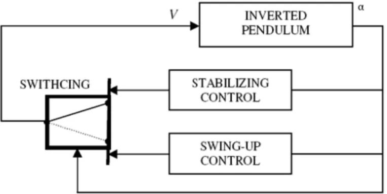
The controller design for the inverted pendulum system is broken up into two components. The first part involves the design of a swing up controller that swings the pendulum up to the unstable equilibrium. The second part involves the design of an optimal state feedback controller that will stabilize the pendulum around the upright position. When the pendulum approaches the linearized point, the control will switch to the stabilizing controller which will balance the pendulum around the vertical position. The control scheme of SESIP consists of two main control loops and a decision making logic to switch between the two control schemes. The control scheme of the

inverted pendulum is shown in Fig. 3. One of the two control loops is a PV controller on the cart position that follows a set point designed to swing up the pendulum from the suspended to the inverted posture [10]. The other control loop is active when the pendulum is around the upright position and consists of a Linear Quadratic Regulator, maintaining the inverted pendulum in vertical position. The primary objective of the LQR scheme is to

- osture. The linear cart

should track a desired (square wave) position set point and at the same time the controller should also minimize the control effort.

Fig. 3. Control scheme of inverted pendulum

The gain of the LQR scheme is tuned to control the inverted pendulum and linear cart system to satisfy the following design requirements.

1.The pendulum angle should be regulated around its upright position and never exceed a 1 degree

deflection.

2.Rise time 2

3.Control effort Vm should be minimum and is not allowed to reach the saturation level.

4. Controller design 4.1 PV Controller

This controller aims at swinging 0_=-1800_{) while keeping the cart travels within}

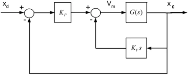
the limited horizontal distance. Many different control algorithms can be used to perform the swing up control such as, trajectory tracking, rectangular reference input swing up type and Pulse Width Modulation (PWM) [11]. In this work, a PV controller is used because of its simple structure, effectiveness and easy tuning. The block diagram representation of swing up controller is shown in Fig. 4. The proportional velocity position controller for servo plant introduces two corrective terms. One is proportional (Kp) to the cart position error while the other is proportional (Kv) to the cart velocity. The resulting PV control law is given as:

(t) ( (t) (t)) d (t)

V_m K_p x_d x_c K_v x_c

dt (20)

The closed loop transfer function of the cart servo can be expressed as:

( ) ( ) ( ) 1 ( ) ( ) K G s x s_c p x_d s K G s_p sK G s_v (21)

This leads to a second order system as follows:

2 (12.23 1.6 ) 1.6 ( ) ( ) s 1.6 K x s_c p x_d s s K_v K_p (22)

The desired performance second order form:

2 ₂ 2 ₀

s _ns _n (23)

Fig. 4. Block diagram of PV controller

4.2 LQR Controller

The LQR method is a powerful technique for designing controllers for complex systems that have stringent performance requirements and it seeks to find the optimal controller that minimizes a given cost function [12]. The cost function is parameterized by two matrices, Q and R, that weight the state vector and the system input respectively. LQR method is based on the state-space model and it tries to obtain the optimal control input by solving the algebraic Riccatti equation. In this paper, the state feedback controller is designed using the linear

quadratic regulator and the linear model of the system. Briefly, the LQR/LTR theory says that, given an nth order

stabilizable system

( ) ( ) ( )

x t Ax t Bu t t 0, x(0) x₀ (24)

Where x t( ) is the state vector and u t( ) is the input vector, determine the matrix K Rn msuch that the static,

full state feedback control law,

( ) ( )

u t Kx t (25)

satisfies the following criteria,

a. the closed-loop system is asymptotically stable b. the quadratic performance functional

and the cost function 1 [ ( ) ( ) ( ) ( )]

2 0

( ) _{x t Qx t u t Ru t dt}T T

J K (26)

is minimized. Q is a nonnegative definite matrix that penalizes the departure of system states from the

equilibrium, and R is a positive definite matrix that penalizes the control input [13]. The following LQR design algorithm is used to determine the optimal state feedback.

Step 1: Solve the matrix Algebraic Riccati Equation(ARE)

PA A P Q PBR B PT 1 T 0 (29)

Step 2: Determine the optimal state x*(t) from

1

*(t) T *( )

x A BR B P x t

(30)

Step 3: Obtain the optimal control u*(t) from

_{u t*( ) R B Px t}1 T _{*( ) (31)} Step 4: Obtain the optimal performance index from

* 1 * ( )T ( )

2

J x t Px t (32) The weighting matrices Q and R are important components of an LQR optimization process. The compositions of Q and R elements have great influences on system performance. The designer is free to select the matrices Q and R, but the selection of matrices Q and R is normally based on an iterative procedure using experience and physical understanding of the problems involved.

5. Experimental Results

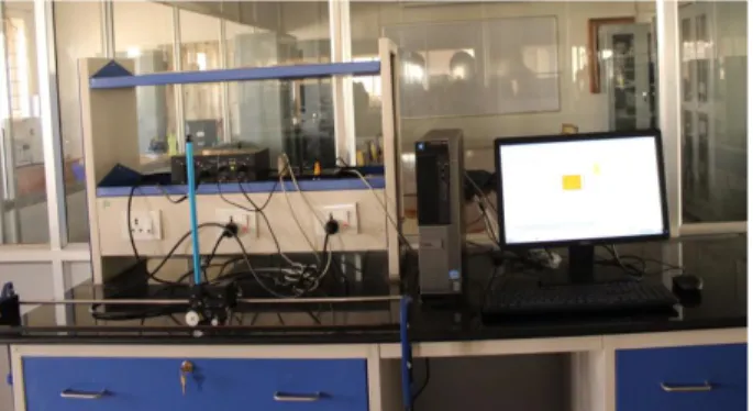
In order to show the practical effectiveness of the proposed scheme, experiments are conducted using Quanser IP-02 inverted pendulum system. The snapshot of the experimental set up is shown in Fig. 5. Firstly, the experimental results of two phases of swing up and stabilizing modes are presented. Secondly, the performance of robust LQR controller design is compared with FSF controller.

Fig. 5. Snapshot of experimental setup

Real time experiment configuration consists of computer with MATLAB, Simulink, Q8 data acquisition board and Quanser IP02 Linear inverted pendulum module. The controller gains of a state feedback controller are determined using the weighting matrices of linear quadratic regulator. The following weighting matrices are selected based on iterative method for the calculation of state feedback gain K.

0.5 0 0 0 0 5.5 0 0 0 0 0 0 0 0 0 0

Q R 0.0003

Using the system model from (18) and the above weighting matrices, the state feedback controller gains obtained for robust LQR controller is

K 44.72 200.8 49.77 27.38 0 5 10 15 20 -200 -150 -100 -50 0 50 100 150 200 Time (sec) P endul um A ngl e ( deg) 0 5 10 15 20 -10 -5 0 5 10 Time (sec) C ont rol s ignal ( vol ts ) Stabilization phase Swing up phase

Fig. 6. Pendulum angle Fig. 7. Control Signal The closed loop poles of the system are found to be

s₁ 6.04 j10.84,s₂ 6.04 j10.84, s₃ 2.97,s₄ 2.10

It can be inferred from the above pole locations that the closed loop system is stable because all the poles are located on the LHP. Fig. 6 shows the output of the swing up controller which is able to bring the pendulum to upright position in around 7 sec. The swing up controller takes approximately 12 swings before the pendulum reaches close to vertical position. During the swing up phase, the magnitude of control signal is larger than that of the stabilizing phase. This is relevant because large amount of energy is required to swing the pendulum from downward position to its upright position and the small amount of energy is only required to stabilize the pendulum. The control signal applied to the cart is shown in Fig. 7. Even though the initial control signal during swing up phase reaches the maximum saturation level, the magnitude of control voltage applied to the motor is reduced well below 3.3V after the pendulum reaches the upright position.

5.1 Disturbance rejection 0 5 10 15 20 25 30 -800 -600 -400 -200 0 200 400 600 800 Time (sec) P endul um V el oc ity ( deg/ s) Disturbance Signal 14.5 15 15.5 16 16.5 17 -80 -60 -40 -20 0 20 40 60 80 Time (sec) P endul um V el oc ity ( deg/ s)

Fig. 8 Pendulum velocity Fig. 9. Zoomed view of pendulum velocity

The disturbance rejection ability of the controller strategy is explained in this section. After the pendulum swing up

and stabilization phase, disturbance is introduced into the pendulum at 15th _{second as shown in Fig. 8. The zoomed}

view of pendulum velocity response is shown in Fig. 9 to highlight the magnitude of deviation in angle. The magnitude of pendulum velocity deviates to a maximum of 60 deg when the disturbance signal is introduced, but the controller is able to reduce the oscillation in less than 2 seconds which makes the pendulum to maintain its upright position to track the given signal.

5.2 Dynamic performance assessment of FSF and LQR controllers

0 5 10 15 20 25 30 -30 -20 -10 0 10 20 30 Time (sec) C ar t di spl ac em ent ( cm ) LQR FSF Reference 0 5 10 15 20 25 30 -1.5 -1 -0.5 0 0.5 1 1.5 Time (sec) P endul um angl e ( deg) FSF LQR Fig.10. Cart position response of FSF and LQR controllers Fig. 11. Pendulum angle response of FSF and LQR controllers Dynamic performance indices such as rise time, settling time and overshoot are chosen to evaluate the performance of both LQR and FSF controllers for the response of cart position and pendulum angle. The state feedback gain f FSF controller is compared with that of the LQR controller. Fig. 10 and 11 show the response of cart position and pendulum angle, respectively. Based on the performance indices given in Table 2, it is worth to note that the LQR controller has less rise time and reaches the set point quickly compare to FSF controller. LQR controller is also characterized by a reduced overshoot and short delay time. In summary, for dynamic response, the inverted pendulum controlled by LQR controller 1) balances faster because of the shorter settling time; 2) has better robustness due to less maximum overshoot. The above points substantiates for the fact that the LQR controller can guarantee the inverted pendulum system a better dynamic performance than a FSF controller.

Table 2. Performance Indices of Cart Position

6. Conclusion

In this paper, a control strategy based on PV controller and robust LQR controller has been proposed for swing up and stabilization of an inverted pendulum. The mathematical model of an inverted pendulum has been obtained using Euler-Lagarangian principles. A PV controller based on energy based method has been implemented to swing up the pendulum to upright position. Once the pendulum reaches the vertical position, a stabilizing controller based on robust LQR is activated to catch the pendulum and to make it track the given reference signal. In order to show the effectiveness of the proposed control scheme, disturbance signal has been introduced into system and the ability of the controller to arrest the oscillation in shorter time period has been experimentally demonstrated. Furthermore, experimental results show that the steady state performance of the proposed LQR controller has smaller oscillation amplitude than that of the FSF controller. The control scheme had not only good dynamic performance, but also robustness to external disturbance. As a future work, in order to further reduce the oscillation amplitude and frequency, friction compensation schemes can be incorporated in the controller strategy.

References

[1] Jia-Jun Wang, 2011.Simulation studies of inverted pendulum based on PID controllers, Simulation Modelling Practice and Theory 19 (2), pp. 440 449.

[2] P. Mason, M. Broucke, B. Piccoli, 2008.Time optimal swing-up of the planar pendulum, IEEE Transactions on Automatic Control 53 (8), pp. 1876 1886.

[3] C.W. Tao, J.S. Taur, T.W. Hsieh, C.L. Tsai, 2008. Design of a fuzzy controller with fuzzy swing-up and parallel distributed pole assignment schemes for an inverted pendulum and cart system, IEEE Transactions on Control Systems Technology 16 (6), pp. 1277 1288.

[4] R. Shahnazi, T.M.R. Akbarzadeh, 2008. PI adaptive fuzzy control with large and fast disturbance rejection for a class of uncertain nonlinear systems, IEEE Transactions on Fuzzy Systems 16 (1), pp. 187 197.

[5] N.A. Chaturvedi, N.H. McClamroch, D.S. Bernstein, 2008. Stabilization of a 3D axially symmetric pendulum, Automatica 44 (9), pp. 2258 2265.

[6] Nenad Muskinja, Boris Tovornik, 2006. Swinging Up and Stabilization of a Real Inverted Pendulum, IEEE Transactions on Industrial Electronics, vol. 53 (2).

[7] A.M. Bloch, D.E Chang, N.E. Leonard, J.E Marsden, 2001. Controlled Lagrangians and the stabilization of mechanical systems II: potential shaping, IEEE Trans. Automatic Control 46 (10), pp. 1556-1571.

[8] K.J. Åström, K. Furuta, 2000. Swinging up a pendulum by energy control, Automatica 36 (2), pp 287 295.

[9] A. A. Saifizul, Z. Zainon, N. A.B. Osman, C. A. Azlan and U. F.S.U. Ibrahim, 2006. Intelligent Control for Self-erecting Inverted Pendulum Via Adaptive Neuro-fuzzy Inference System, American Journal of Applied Sciences, vol 3(4).

[10] Mahmud Iwan Solihin, Rini Akmeliawati, 2010. Particle SwamOptimization for Stabilizing Controller of a Self-erecting Linear Inverted Pendulum, International Journal of Electrical and Electronic Systems Research, Vol 3, pp.410-415.

[11] Wende Li, Hui Ding, Kai Cheng, 2012. An Investigation on the Design and Performance Assessment of double-PID and LQR Controllers for the Inverted Pendulum , UKACC International Conference on Control.

[12] Aamir New Approach for Position Control of Induction motor 45th _{Universities Power}

Engineering Conference.

[13] Desineni Subbaram. Naidu, 2003. Optimal Control Systems, CRC press. [14] Quanser Inc., Canada, 2006 . Inverted pendulum plant manual.

Time domain parameter FSF LQR

Rise time (sec) 3.1 1.8

Settling time (sec) 3.8 3.2