Kernel-Based Semiparametric Estimators: Small Bandwidth
Asymptotics and Bootstrap Consistency
∗Matias D. Cattaneo† Michael Jansson‡ April 16, 2018
Abstract
This paper develops asymptotic approximations for kernel-based semiparametric estimators under assumptions accommodating slower-than-usual rates of convergence of their nonpara-metric ingredients. Our first main result is a distributional approximation for semiparanonpara-metric estimators that differs from existing approximations by accounting for a bias. This bias is non-negligible in general, and therefore poses a challenge for inference. Our second main result shows that some (but not all) nonparametric bootstrap distributional approximations provide an automatic method of correcting for the bias. Our general theory is illustrated by means of examples and its main finite sample implications are corroborated in a simulation study.
Keywords: semiparametrics, small bandwidth asymptotics, bootstrapping, robust inference.
JEL: C12, C14, C21.
∗A previous version of this paper was circulated under the title “Bootstrapping Kernel-Based Semiparametric
Estimators”. We thank Elie Tamer, four referees, Stephane Bonhomme, Lutz Kilian, Xinwei Ma, Whitney Newey, Jamie Robins, Adam Rosen, Andres Santos, Azeem Shaikh, Xiaoxia Shi, and seminar participants at Cambridge University, Georgetown University, London School of Economics, Oxford University, Rice University, University of Chicago, University College London, University of Michigan, the 2013 Latin American Meetings of the Econometric Society, and 2014 CEME/NSF Conference on Inference in Nonstandard Problems for comments. The first author gratefully acknowledges financial support from the National Science Foundation (SES 1122994 and SES 1459931). The second author gratefully acknowledges financial support from the National Science Foundation (SES 1124174 and 1459967) and the research support of CREATES (funded by the Danish National Research Foundation under grant no.
†Department of Economics and Department of Statistics, University of Michigan. ‡Department of Economics, UC Berkeley andCREATES.
1
Introduction
The importance of semiparametric estimators is widely recognized, yet the consensus opinion seems to be that existing large sample results suffer from the serious shortcoming that the finite sample distributions of these estimators are much more sensitive to the properties of their (slowly converg-ing) nonparametric ingredients than conventional asymptotic theory would suggest. In other words, the conventional approach to asymptotic analysis of semiparametric estimators, while delivering very tractable distributional approximations, effectively ignores certain features of these estimators that are important in samples of realistic size. Motivated by this observation, and with the ultimate goal of developing more “robust” inference procedures based on semiparametric estimators, this paper obtains two main results. (We employ a certain well-defined sense of “robustness” discussed precisely below.)
First, we revisit the large sample properties of kernel-based semiparametric estimators and ob-tain novel distributional approximations for members of this large class. By design, these approxi-mations capture certain features of their nonparametric ingredient that are ignored by conventional approximations. Moreover, as a consequence of their method of construction, our approximations are demonstrably more robust than conventional ones in the sense that we allow for (but do not re-quire) nonparametric ingredients whose precision is low enough (in an order of magnitude sense) to render conventional distributional approximations invalid. Accordingly, our approximations lead to an improved understanding of the finite and large sample properties of semiparametric estimators. Relative to conventional approximations, the distinguishing feature of the distributional approx-imations developed herein is that they explicitly account for the presence of a (possibly) first-order bias effect, which emerges when the precision of the first-step nonparametric estimator is sufficiently low. The presence of the bias unearthed by our first main result poses potentially serious challenges
for inference: for instance, the commonly used “estimator ± 1.96 × standard error” approach to
construct an approximate 95% confidence interval for a scalar parameter of interest is invalid in the presence of a non-negligible bias. Nonetheless, our second main result shows that a carefully implemented nonparametric bootstrap distributional approximation provides an automatic method of bias correction and that the associated percentile confidence intervals are asymptotically valid even in the presence of a non-negligible bias. In addition to being of theoretical interest, this result therefore offers guidance for empirical work.
For the semiparametric estimators we consider, the precision of the nonparametric ingredi-ent is governed by the bandwidth associated with the kernel-based first-step estimator. In the development of our results, we use this bandwidth as a technical device to shed light on the in-terplay between the distributional properties of the semiparametric estimator and the precision of its nonparametric ingredient. In particular, because the rate of convergence of the nonparametric ingredient is low when the bandwidth is “small”, the bandwidths for which our results offer new insights are those that are small and we therefore use the term “small bandwidth asymptotics” to highlight the distinguishing feature of the technical approach we take in this paper. This termi-nology is consistent with that used in earlier work of ours, but in important respects the results
obtained herein differ from those currently available in the literature.
Cattaneo, Crump, and Jansson (2010, 2014a) study the density-weighted average derivative
estimator of Powell, Stock, and Stoker (1989) and show that the distinguishing feature emerging
from the small bandwidth distributional approximation for that particular estimator is the presence
of a variance effect, while Cattaneo, Crump, and Jansson (2014b) show that the variance effect in
question cannot be corrected for by using the standard nonparametric bootstrap. In contrast, this paper is concerned with a class of estimators for which the distinguishing feature of their small bandwidth asymptotic distribution is the presence of a bias effect. A well-known member of the class of estimators studied in this paper is the weighted average derivative estimator analyzed in
Cattaneo, Crump, and Jansson(2013) and, as a consequence, our first main result can be interpreted as a nontrivial generalization of one of the results in that paper, since the results herein cover a large class of two-step (possibly over-identified and non-differentiable) GMM settings. Furthermore, our second main result offering bootstrap-based automatic bias reduction and valid inference appears to be new in the literature.
At a conceptual level, our small bandwidth approach is very similar to the “dimension
asymp-totics” approach taken in the seminal work of Mammen(1989) and, although the technical details
are rather different, some of our main conclusions are similar to his. For a more detailed explana-tion of the connecexplana-tion between small bandwidth asymptotics and dimension asymptotics, see Enno
Mammen’s discussion ofCattaneo, Crump, and Jansson(2013). The approach we take is also
sim-ilar to the approach taken by Abadie and Imbens(2006,2008), but our main conclusion regarding
the bootstrap (and subsampling) is quite different from that of Abadie and Imbens (2008).
The literature on two-step semiparametric estimators is vast, but our first main result differs from most existing results in at least two respects. First, due to the presence of a bias, our
distri-butional conclusions differ from those obtained in the work surveyed by Andrews (1994b), Newey
and McFadden (1994), Chen (2007), and Ichimura and Todd (2007). Second, a seemingly novel technical feature of our work is that reliance on a heretofore ubiquitous stochastic equicontinuity condition is avoided and that avoiding such condition is necessary, in general, in order for the bias we highlight to be non-negligible; that is, our generalization of existing distributional conclusions cannot be accomplished without avoiding reliance on a stochastic equicontinuity condition that has featured prominently in earlier work.
Our second main result concerns the bootstrap. Previous work on bootstrap validity for
gen-eral classes of semiparametric models under standard conditions includes Chen, Linton, and van
Keilegom(2003) andCheng and Huang (2010). Our result is qualitatively similar to the bootstrap consistency results of these papers, but in at least two respects our results broaden the scope of resampling-based inference in a possibly surprising way. First, we show that some (but not all) standard bootstrap-based distributional approximations deliver an automatic bias correction. Sec-ond, whereas all previous bootstrap consistency results have been obtained for settings in which subsampling-based inference procedures are also valid, the bias effect that is central to our work turns out to render subsampling-based inference procedures invalid in general. To the extent that
subsampling can be regarded as a “regularized” version of the bootstrap (e.g., Bickel and Li,2006), it therefore seems surprising that the standard nonparametric bootstrap in its simplest form turns out to be asymptotically valid in the setting of this paper.
Other work related to ours includes Chernozhukov, Escanciano, Ichimura, and Newey (2016)
and Robins, Li, Tchetgen, and van der Vaart (2008). When specialized to kernel-based
estima-tors, the local robustness property discussed by Chernozhukov, Escanciano, Ichimura, and Newey
(2016) can be interpreted as an application of “large bandwidth asymptotics” and their results are
complementary to ours in the sense that they ensure robustness to “large” bandwidths by paying more careful attention to the smoothing bias that our theory is largely silent about. The work on
higher-order influence functions by Robins, Li, Tchetgen, and van der Vaart (2008) is similar to
ours at least insofar as its uses higher-order U-statistics and focuses on settings where
nonpara-metric ingredients converge at slow rates, but unlike us they focus on problems for which optimal interval estimates exhibit a slower-than-usual rate of convergence and even when specialized to the
average density example studied below the results obtained using their approach (e.g., Robins, Li,
Tchetgen, and van der Vaart, 2016; Robins, Li, Mukherjee, Tchetgen, and van der Vaart, 2017) appears to be quite different from ours.
The paper proceeds as follows. Section 2 introduces the setup and gives our first main result.
Section 3 gives an in-depth discussion of that result, including both connections to previous
the-oretical work on semiparametrics and implications for empirical work employing semiparametric
inference procedures. Section 4 presents our second main result, a bootstrap analog of the main
result from Section 2. Section5is concerned with generic verification of the high-level assumptions
under which our main results are obtained, while Section 6 illustrates how the latter sufficient
conditions for our high-level assumptions can be verified in the context of the specific example of inverse probability weighting (IPW) estimation with possibly non-differentiable moment functions.
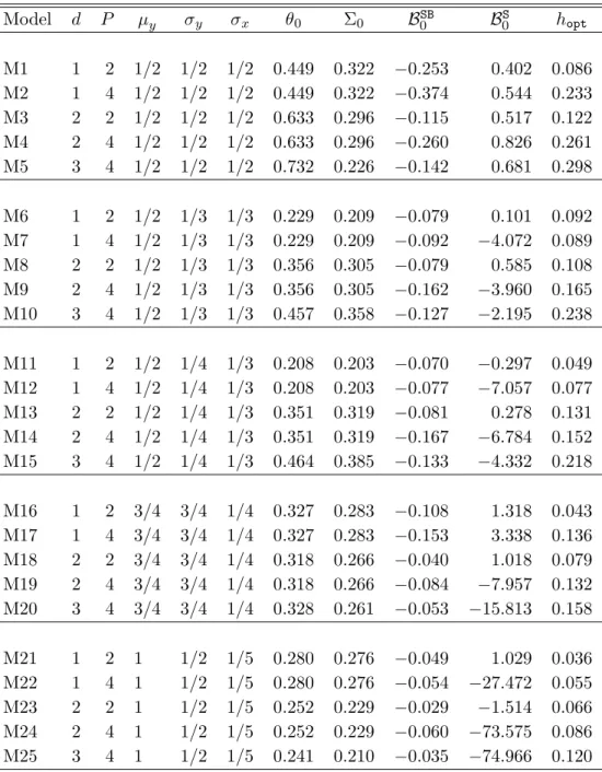
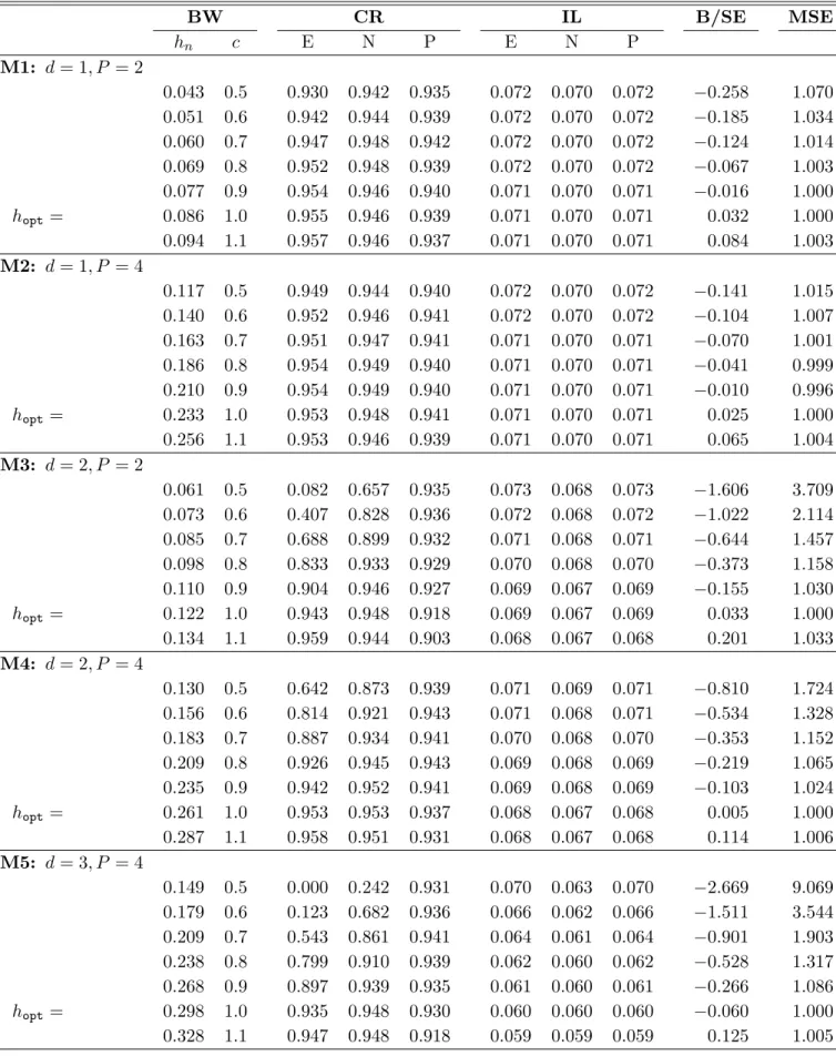
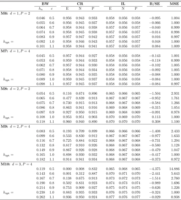
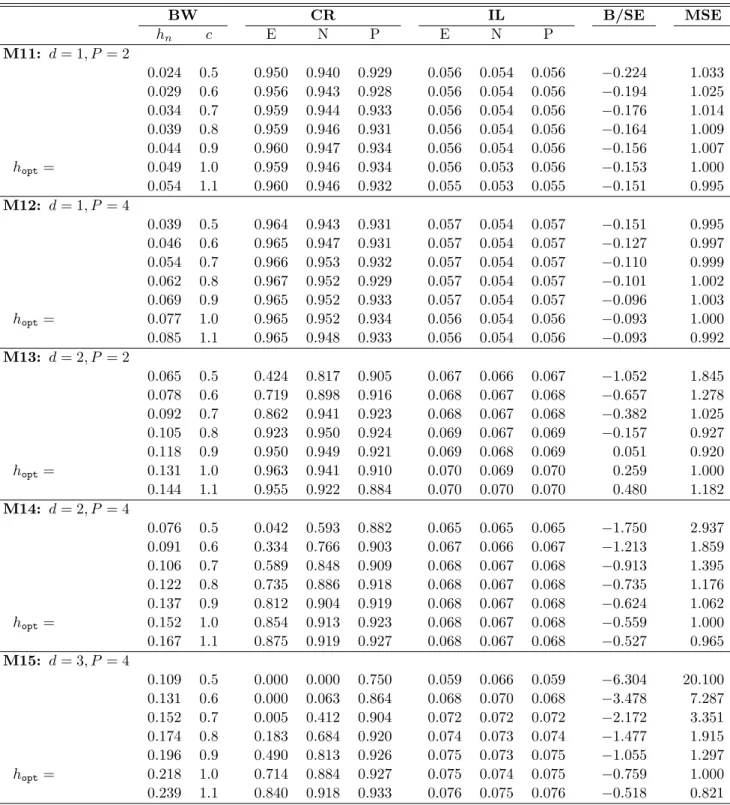
Finally, Section 7 offers simulation evidence, and Section 8 concludes.
Three distinct examples are considered in the paper. The first of these is mainly pedagogical and serves the dual purposes of illustrating our main results in a canonical setting while at the same time demonstrating the fact that the complications we highlight are present even in the simplest of examples. Our second example, the IPW example already mentioned, is more substantive and a representative member of a class of estimators which is very popular in a variety of settings in ap-plied work, including program evaluation, missing data, measurement error, and data combination. Finally, the simulation results make use of an estimator which is easy to compute, yet somewhat challenging to analyze and base inference on, namely a so-called “Hit Rate” estimator. Technical details for all three examples are provided in the supplemental appendix, which also contains some additional technical results that may be of independent interest.
2
Kernel-Based Semiparametric Estimators
Suppose θ0 ∈Θ⊆Rdθ is an estimand representable as the solution (with respect to θ ∈Θ) to an
equation of the form
G(θ, γ0) = 0, G(θ, γ) =Eg(z, θ, γ),
where g is a known functional, z is a random vector, and γ0 is an unknown function. Letting
z1, . . . , zn denote i.i.d. copies of z and assuming that ˆγn is a nonparametric estimator of γ0, a
natural estimator ˆθn of θ0 is given by a minimizer (with respect to θ∈Θ) of
ˆ Gn(θ,γˆn)0WˆnGˆn(θ,γˆn), Gˆn(θ, γ) = 1 n n X i=1 g(zi, θ, γ),
where ˆWn is some (possibly random) symmetric, positive semi-definite matrix.
Estimators of this kind, often referred to as semiparametric two-step estimators, are widely used in practice and have received considerable attention in the literature. A common feature of existing distributional results for semiparametric two-step estimators, including those surveyed by
Andrews (1994b), Newey and McFadden (1994), Chen (2007) and Ichimura and Todd (2007), is
that they are developed under assumptions ensuring that the limiting distribution of ˆθn depends
on ˆγn only through the estimand γ0.To be specific, existing asymptotic results are of the form
√
n(ˆθn−θ0) N(0,Σ0), (1)
where denotes weak convergence and where it follows from Newey (1994a, Proposition 1) that
the asymptotic variance Σ0 depends on ˆγn only through its probability limit (under general
mis-specification) and not on the method used to construct ˆγn (e.g., kernels, local polynomials, or
series) and/or on the value of the “tuning” parameter(s) associated with the chosen method (e.g., the kernel and the bandwidth for kernel estimators). While the simplicity of the limiting
distribu-tion in (1) is desirable insofar as it facilitates inference on θ0,the rather extreme insensitivity of
this distributional approximation with respect to the specifics of the nuisance parameter estimator ˆ
γn is arguably unsatisfactory because folklore and simulation evidence suggests that in samples of
realistic size the distributional properties of ˆθndo in fact depend somewhat heavily on the specifics
of ˆγn.
The insensitivity of the distributional conclusion (1) with respect to the specifics of the first-step
estimator ˆγn is driven in large part by assumptions ensuring that ˆγnconverges sufficiently rapidly
toγ0.To be specific, assumptions of the form ˆγn−γ0 =oP(n−1/4) are ubiquitous in the literature
on semiparametric two-step estimators and the simplicity of (1) is largely due to these convergence
rate assumptions. As a means to the end of developing more reliable distributional approximations
for ˆθn,this paper allows for (but does not require) milder-than-usual convergence rate requirements
on ˆγn as a theoretical device to obtain distributional approximations for semiparametric
some of the specific features underlying the estimator ˆγn. Therefore, unlike conventional
approx-imations currently available in the literature, our distribution theory for two-step semiparametric estimators is able to explicitly account for the effect of the first-step estimator on the distributional approximation. More specifically, we obtain results of the form
√
n(ˆθn−θ0−Bn) N(0,Σ0), (2)
where Σ0 is the usual asymptotic variance of a semiparametric estimator (i.e., the same as in (1))
and Bn is a non-random “bias” term. Because the distribution theory developed herein is
consis-tent with conventional results when the latter are applicable, the bias Bn in (2) is asymptotically
negligible (i.e., o(n−1/2)) under conventional assumptions, but in general Bn turns out to be
non-negligible under seemingly mild departures from those assumptions. Moreover, the magnitude and
functional form ofBnturns out to depend on the specifics of the estimator ˆγnused in the
construc-tion of ˆθn.In other words, we find that although the asymptotic variance of ˆθnremains insensitive
with respect to the type of first step nonparametric estimator also under our (weaker) assumptions,
the specific structure of ˆγndoes exert a first-order effect on ˆθnthroughBn when milder-than-usual
convergence rate requirements are placed on ˆγn.
The result (2) follows from three easy-to-interpret high-level conditions in the important special
case where the first-step estimator ˆγn is kernel-based in the sense that
ˆ γn= (ˆγn,1, . . . ,γˆn,dγ)0, γˆn,k(z, θ) = 1 n n X j=1 wk(zj, θ)κn,k[xk(z, θ)−xk(zj, θ)], (3) whereκn,k(x) =κk(x/hn,k)/hdk
n,k, hn,k=o(1) is a bandwidth, κk is a (kernel-like) function, and wk
andxk are known functions of dimensions one anddk,respectively. Nonparametric estimators that
can be written in the form (3) include kernel estimators (e.g., of the form discussed by Newey and
McFadden, 1994, Section 8.3) and local polynomial regression estimators (e.g., Fan and Gijbels,
1997). On the other hand, series estimators are not of this form, and we therefore use the term
“kernel-based” when referring to the estimator in (3).
Our first high-level condition is the following.
Condition AL (Approximate Linearity) For some non-random Jn and J0,Jn→ J0 and ˆ
θn−θ0 =JnGˆn(θ0,ˆγn) +oP(n−1/2).
Condition AL is referred to as “approximate linearity” in recognition of the fact that the
condi-tion effectively approximates ˆGn(θ, γ) with a function that is linear/affine with respect to θ.In
par-ticular, Condition AL is simply a representation, the displayed equality holding with Jn=J0 =Idθ
and without anyoP(n−1/2) term, in the important special case whereg(z, θ, γ) =g(z,0, γ)−θand ˆθn is defined as the solution to ˆGn(θ,ˆγn) = 0.More generally, standard heuristics suggest that, under
˙
G0 = ∂G(θ, γ0)/∂θ0
θ=θ0 and whereW0 is the probability limit of ˆWn.Lemma1below gives
condi-tions under which these heuristics can be made rigorous also when ˆγn exhibits a slower-than-usual
rate of convergence.
Under Condition AL, the large sample properties of ˆθnare governed by
ˆ Gn(θ0,γˆn) = 1 n n X i=1 g0(zi,γˆn), g0(z, γ) =g(z, θ0, γ).
Analyzing this object without assuming a faster-than-n1/4 rate of convergence on the part of ˆγn
turns out to be challenging partly because the standard method of accounting for the
depen-dence/overlap between the arguments zi and ˆγn of the summandg0(zi,γˆn) turns out to be invalid
when ˆγn converges at a slower-than-usual rate. Specifically, as further discussed and exemplified in
Section 3.1, it turns out that a commonly employed stochastic equicontinuity condition typically
requires (and/or is applicable only when one assumes) that the rate of convergence of ˆγn exceeds
n1/4.
Analyzing ˆGn(θ0,γˆn) without imposing further structure on g and/or relying on stochastic
equicontinuity nevertheless turns out to be feasible when ˆγn is kernel-based, the reason being that
in this case ˆGn(θ0,ˆγn) admits a representation of the form ˆ Gn(θ0,γˆn) = 1 n n X i=1 gn(zi,γˆ(ni)), (4)
wheregn is some function and where
ˆ γn(i)= (ˆγn,(i)1, . . . ,ˆγ(n,di) γ) 0, γˆ(i) n,k(z, θ) = 1 n−1 n X j=1,j6=i wk(zj, θ)κn,k[xk(z, θ)−xk(zj, θ)],
is the ith “leave-one-out” estimator of γ0.To be specific, the fact that ˆγn is kernel-based implies
that each ˆγn,k is additively separable between zi and {zj :j6=i}: ˆ
γn,k(z, θ) =n−1ˆγin,k(z, θ) + (1−n−1)ˆγ(n,ki)(z, θ),
where
ˆ
γin= (ˆγin,1, . . . ,γˆn,di γ)0, ˆγin,k(z, θ) =wk(zi, θ)κn,k[xk(z, θ)−xk(zi, θ)]. As a consequence, the function
gn(zi, γ) =g0(zi, n−1γˆin+ (1−n−1)γ)
satisfiesgn(zi,ˆγ(ni)) =g0(zi,ˆγn),implying in particular that the representation (4) is valid.
In addition to delivering (4), the assumption that ˆγn is kernel-based makes it possible to
Condition AS (Asymptotic Separability) For some ˉgn, 1 √ n n X i=1 [gn(zi,ˆγn(i))−gn(zi, γn)] = 1 √ n n X i=1 [ˉgn(zi,γˆ(ni))−ˉgn(zi, γn)] +oP(1), = √1 n n X i=1 [ ˉGn(ˆγ(ni))−Gˉn(γn)] +oP(1), whereγn(∙) =Eγˆn(∙) and ˉGn(γ) =Eˉgn(z, γ).
The main part of Condition AS is the second equality and the function ˉgn is introduced to
facilitate verification of that part (and of Condition AN below). Indeed, while the first part of
Condition AS holds (without any oP(1) term) when ˉgn = gn, the second part of Condition AS
is considerably easier to verify when ˉgn(z,∙) is a low-order polynomial approximation to gn(z,∙).
When the rate of convergence of ˆγnexceedsn1/6(but not necessarilyn1/4), the simplest polynomial
approximation to gn(z,∙) satisfying the first part of Condition AS is usually a quadratic one of the
form
ˉ
gn(z, γ) =gn(z, γn) +gn,γ(z)[γ−γn] + 1
2gn,γγ(z)[γ−γn, γ−γn], (5)
wheregn,γ(z)[∙] and gn,γγ(z)[∙,∙] are linear and bilinear functionals, respectively. Conditions under
which the second part of Condition AS is satisfied when ˉgnis of the form (5) will be given in Lemma
2 below.
Condition AS implies that the separable (between zi and ˆγ(ni)) approximation
gn(zi,ˆγn(i))≈gn(zi, γn) + ˉGn(ˆγn(i))−Gˉn(γn) togn(zi,ˆγ(ni)) is asymptotically valid in the sense that it satisfies
√ nGˆn(θ0,ˆγn) = 1 √ n n X i=1 gn(zi,γˆ(ni)) = 1 √ n n X i=1 [gn(zi, γn) + ˉGn(ˆγn(i))−Gˉn(γn)] +oP(1). (6)
Because averages of terms (such as gn(zi, γn) and ˉGn(ˆγ
(i)
n )−Gˉn(γn)) that each depend on one, but not both, ofzi and ˆγ(ni)are much easier to analyze than averages of terms (such as gn(zi,γˆ(ni))) that depend on both zi and ˆγ(ni),Condition AS therefore greatly simplifies the analysis of ˆGn(θ0,γˆn).
In addition to the notational nuisance of having to employ additional sub- and super-scripts in many places, a more substantive complication that must be addressed when proceeding under
Condition AS is that it turns out that the leading term in (6) has a nonnegligible mean in general.
Whereas the limiting distribution of √nGˆn(θ0,ˆγn) is normal with mean zero under conventional
asymptotics, the simplest asymptotic normality result about the leading term in (6) that one can
hope for more generally is therefore the following, primitive sufficient conditions for which will be
Condition AN (Asymptotic Normality) For some non-random Bn and Ω0, 1 √ n n X i=1 [gn(zi, γn) + ˉGn(ˆγ(ni))−Gˉn(γn)− Bn] N(0,Ω0).
Combining Conditions AL, AS, and AN, we obtain (2). For later reference, we state this
observation as a theorem.
Theorem 1 If ˆγn is kernel-based and if Conditions AL, AS, and AN are satisfied, then (2) holds with Σ0 =J0Ω0J00 andBn=JnBn.
3
Discussion of Theorem
1
Theorem1differs in three important ways from existing “master theorems” concerning the
asymp-totic distribution of semiparametric two-step estimators. First, although the high-level assumptions
of Theorem 1 look remarkably similar to their natural counterparts in the existing literature, our
Assumption AS differs in a subtle, yet crucial, way from a heretofore ubiquitous stochastic
equicon-tinuity assumption. Second, Theorem 1 sheds new light on the bias properties of semiparametric
two-step estimators. Finally, and perhaps most interestingly from the perspective of empirical
practice, Theorem 1 has important implications for inference. The following subsections discuss
these three differences in turn and illustrates them by means of the following canonical example.
Example 1: Average Density. Supposez1, . . . , zn arei.i.d.copies of a continuously distributed
random vectorz∈Rdwith a densityγ
0.Then a kernel-based estimator ofθ0 =Eγ0(z),the average
density, is given by ˆ θADn = 1 n n X i=1 ˆ γn(zi), γˆn(z) = 1 n n X j=1 Kn(z−zj), where Kn(z) = K(z/hn)/hd
n, hn is a bandwidth, and K is a kernel. The estimator ˆθ
AD
n can be
interpreted as the solution to ˆGn(θ,γˆn) = 0,where
g(z, θ, γ) =gAD(z, θ, γ) =γ(z)−θ.
Under standard regularity conditions (e.g., those given in Section SA.1 of the Supplementary Ap-pendix), ˆθADn can be analyzed using the results of this paper, as can the related estimators ˆθISDn and
ˆ
θLRn introduced below.
3.1 Asymptotics without Stochastic Equicontinuity
In the existing semiparametrics literature, the analysis of objects such as ˆGn(θ0,γˆn) invariably
Condition SE (Stochastic Equicontinuity) For some ˉg0, 1 √ n n X i=1 [g0(zi,γˆn)−g0(zi, γ0)] = 1 √ n n X i=1 [ˉg0(zi,ˆγn)−gˉ0(zi, γ0)] +oP(1), = √1 n n X i=1 [ ˉG0(ˆγn)−Gˉ0(γ0)] +oP(1), where ˉG0(γ) =Egˉ0(z, γ).
Like Condition AS, Condition SE is an “asymptotic separability” condition insofar as it implies
that the separable (between zi and ˆγn) approximation
g0(zi,ˆγn)≈g0(zi, γ0) + ˉG0(ˆγn)−Gˉ0(γ0)
tog0(zi,γˆn) is asymptotically valid in the sense that
√ nGˆn(θ0,γˆn) = 1 √ n n X i=1 g0(zi,ˆγn) = 1 √ n n X i=1 [g0(zi, γ0) + ˉG0(ˆγn)−Gˉ0(γ0)] +oP(1).
We refer to the condition using the label “SE” because the second (and main) part of the condition
reduces to well known stochastic equicontinuity conditions for suitable choices of ˉg0.In particular,
the second part of Condition SE reduces to Assumption 5.2 ofNewey(1994a) when ˉg0(z, γ) is linear
inγ and to (2.8) ofAndrews (1994a) and (3.34) of Andrews (1994b) when ˉg0=g0.
On the surface, Condition AS might appear to be nothing more than a “leave-one-out” coun-terpart of Condition SE. Crucially, however, the primitive conditions required to verify the second parts of AS and SE can often differ significantly.
Example 1 (continued). Turning first to Condition AS and setting ˉgAD
n = gnAD, the first part of that condition is automatically satisfied and the second part becomes
1 √ n n X i=1 [ˆγ(ni)(zi)−2γn(zi) +θn] =oP(1), where ˆ γ(ni)(z) = 1 n−1 n X j=1,j6=i Kn(z−zj), γn(∙) =Eγˆn(∙), θn=Eγn(z).
It follows from a simple variance calculation that Condition AS is satisfied if nhdn→ ∞.
On the other hand, setting ˉgAD
0 = gAD0 the first part of Condition SE is automatically satisfied
and the second part becomes 1 √ n n X i=1 [ˆγn(zi)−γn(zi)−γ0(zi) +θ0] =oP(1).
It follows from a direct calculation that if nhdn→ ∞,then 1 √ n n X i=1 [ˆγn(zi)−γn(zi)−γ0(zi) +θ0] = 1 p nh2d n K(0) +oP(1),
so Condition SE requires the stronger condition nh2nd→ ∞ unlessK(0) = 0.
To interpret the bandwidth requirements nhd
n→ ∞and nh2nd→ ∞ associated with Conditions
AS and SE in this example it is helpful to recall that the (pointwise) rate of convergence of ˆγn−γn
is pnhd
n; that is, ˆγn(z)−γn(z) = OP(1/ p
nhd
n) for any z ∈ Rd. The conditions nhdn → ∞ and
nh2d
n → ∞ therefore correspond loosely to the requirements of consistency and faster-than-n1/4
-consistency, respectively, on the part of the nonparametric ingredient ˆγn.
Although exceedingly simple in some respects, the average density example is representative
in the sense that while the second part of Condition AS typically holds whenever ˆγn is consistent
(in a suitable sense), the second part of Condition SE typically requires ˆγn to be
faster-than-n1/4-consistent. As a consequence, reliance on Condition SE must be avoided, in general, when
accommodating nonparametric components whose convergence rate is no faster than n1/4. More
importantly, perhaps, the average density example illustrates the fact that reliance on Condition SE
must be avoided, in general, when the goal is to generalize (1), as the termK(0)/pnhd
nquantifying
the departure from Condition SE turns out to be the main source of the bias of the average density estimator.
In other words, in addition to being an interesting technical challenge that can be motivated by the desire to accommodate nonparametric components whose convergence rate is no faster than
n1/4,relaxing Condition SE is of fundamental importance when the goal is to obtain more refined
distributional approximations than (1). We are unaware of previous work pointing out the need
to, let alone providing a solution to the question of how to, avoid reliance on Condition SE (or the
like) when generalizing (1) and/or accommodating nonparametric components whose convergence
rate is no faster than n1/4. Our proposed Condition AS is arguably an attractive alternative to
Condition SE because it inherits one of the main benefits of the conventional Condition SE (namely,
“asymptotic separability”) without imposing unduly strong convergence rate requirements on ˆγn.
A drawback of Condition AS in its present formulation is that ˆγn is assumed to be kernel-based.
Although doing so is beyond the scope of the present paper, it would be of interest to relax that assumption.
We are aware of only two exceptions to the rule that Condition SE requires ˆγnto be
faster-than-n1/4-consistent. The first of these exceptions occurs when g0(zi, γ) and gn(zi, γ) coincide (apart from a non-important factor of proportionality). An important example of this phenomenon is
provided by the “leave in” version of Powell, Stock, and Stoker’s (1989) estimator: As pointed out
in their footnote 6, that estimator satisfies g0(zi, γ) = (1−n−1)gn(zi, γ) because symmetric kernels
z and γ, as is the case for the consumer surplus estimator of Hausman and Newey (1995) where
the associated g0(z, γ) does not depend on z at all. Both exceptions can be illustrated by means
of Example 1.
Example 1 (continued). The functiongAD
0 satisfiesg0AD(zi, γ) = (1−n−1)gnAD(zi, γ) whenK(0) = 0, so in this case Condition SE holds whenever Condition AS does.
An alternative estimator of θ0=RRdγ0(u)2duis the integrated squared density estimator
ˆ θISDn = Z Rd ˆ γn(u)2du,
which can be interpreted as the solution to ˆGn(θ,ˆγn) = 0,where g(z, θ, γ) =gISD(z, θ, γ) = Z Rd γ(u)2du−θ. Because gISD 0 (z, γ) = R
Rdγ(u)2du−θ0 does not even depend on z, (asymptotic) “separability”
between z and γ is of course automatic and, indeed, both parts of Condition SE are satisfied
(without any oP(1) terms) when ˉgISD
0 =g0ISD.(Setting ˉgISDn = gISDn and applying Lemma 2 below,
Condition AS can also be shown to hold provided nhd
n→ ∞.) 3.2 Bias Properties
Under the conditions of Theorem 1, the main determinant of the bias Bn in (2) is Bn of Condition
AN. When Condition AS is satisfied with a ˉgn of the form (5), the functional ˉGn is also quadratic.
Indeed, defining Gn(γ) =Egn(z, γ), Gn,γ[η] =Egn,γ(z)[η], Gn,γγ[η, ϕ] =Egn,γγ(z)[η, ϕ], we have ˉ Gn(γ) =Gn(γn) +Gn,γ[γ−γn] + 1 2Gn,γγ[γ−γn, γ−γn].
Because ˆγi,n−γn has mean zero, the leading term in (6) therefore satisfies
E[gn(zi, γn) + ˉGn(ˆγ(ni))−Gˉn(γn)] =BnS +BLIn +BNLn, where
BnS =G0(γn), G0(γ) =Eg0(z, γ),
is a “smoothing” bias term, while
BLI n =Gn(γn)−G0(γn) and BnNL= 1 2nEGn,γγ[ˆγ i n−γn,γˆin−γn]
are generic versions of what Cattaneo, Crump, and Jansson (2013) refer to as “leave in” and “nonlinearity” bias terms, respectively.
The smoothing bias BS
n is familiar from the conventional theory and we have nothing new to
say about it, but because one of our main results (namely, Theorem 2 below) effectively requires
the smoothing bias to be asymptotically negligible (i.e., BS
n =o(n−1/2)) we give a brief discussion
of sufficient conditions for this to occur. In most cases the magnitude of BS
n coincides with that of
the smoothing bias γn−γ0 of the first-step estimator ˆγn,leading to the familiar conclusion that
undersmoothing is required in order to achieveBS
n=o(n−1/2).An exception to this rule might occur
when the moment function g(z, θ, γ) is “locally robust” in the sense of Chernozhukov, Escanciano,
Ichimura, and Newey (2016), as ˆθn then has the “small bias property” discussed byNewey, Hsieh,
and Robins (2004); i.e., the magnitude of BS
nis smaller than that of γn−γ0.
Example 1 (continued). The bias γn −γ0 of ˆγn satisfies RRd[γn(u)−γ0(u)]2du = O(h2nP),
ashn→0,whereP is the order of the kernel K.As a consequence,
GAD0 (γn) =
Z
Rd
[γn(u)−γ0(u)]γ0(u)du=O(hPn),
so the smoothing bias associated with ˆθADn is asymptotically negligible provided nh2P
n → 0, a
condition which requires undersmoothing because the MSE-optimal bandwidth for ˆγn satisfies
hn∼n−1/(2P+d).
The condition for the smoothing bias associated with ˆθISDn to be asymptotically negligible is the
same as that for ˆθADn,the reason being that GISD0 (γn) = 2GAD0 (γn) +
Z
Rd
[γn(u)−γ0(u)]2du= 2GAD0 (γn) +O(h2nP).
On the other hand, the estimator ˆ θLRn = 2ˆθADn −ˆθISDn = 2 n n X i=1 ˆ γn(zi)− Z Rdˆ γn(u)2du
has the small bias property, as it can be interpreted as the solution to ˆGn(θ,γˆn) = 0 with g(z, θ, γ) =gLR(z, θ, γ) = 2gAD(z, θ, γ)−gISD(z, θ, γ) = 2γ(z)−
Z
Rd
γ(u)2du−θ,
wheregLR is locally robust because it follows from the foregoing that
GLR0 (γn) =−
Z
Rd
[γn(u)−γ0(u)]2du=O(h2nP).
As a consequence, the smoothing bias associated with ˆθLRn is asymptotically negligible provided
The leave-in and nonlinearity biases are usually asymptotically negligible whenever the rate of
convergence of ˆγn exceeds n1/4. As a consequence, these biases play no role in the conventional
theory. In contrast, it turns out that one or both of BLI
n and BNLn will typically be nonnegligible
when the rate of convergence of ˆγn is no faster than n1/4.To be specific, when ˆγ
n−γn6=oP(n1/4)
one typically finds that BLI
n is nonnegligible whenever Condition SE fails while BnNLis nonnegligible
whenever g0(z, γ) is nonlinear in γ. Example 1 (continued). Because
GADn(γn)−GAD0 (γn) = 1 nhd
n
K(0) +O(n−1),
the leave-in bias associated with ˆθADn is nonnegligible unless either nh2d
n → ∞ or K(0) = 0, the
former being the condition under which the rate of convergence of ˆγn exceeds n1/4 and the latter
being the condition under which Condition SE is satisfied by gAD. On the other hand, because
gAD
0 (z, γ) = γ(z)−θ0 is linear in γ, GADn,γγ[∙,∙] = 0 and the nonlinearity bias associated with ˆθ
AD
n is
zero. In summary, we therefore find that if nh2nP →0 and ifnhdn→ ∞,then
E[gnAD(zi, γn) + ˉGADn(ˆγ(ni))−GˉADn (γn)] =BADn +o(n−1/2), BADn = 1
nhd n
K(0).
When nhdn→ ∞,Condition SE is satisfied by gISD and the leave-in bias associated with ˆθISD
n is negligible because
GISDn (γn)−G0ISD(γn) =O(n−1).
On the other hand, because gISD
0 (z, γ) =
R
Rdγ(u)2du−θ0 is nonlinear in γ, the nonlinearity bias
associated with ˆθISDn is nonzero. Indeed, EGISDn,γγ[ˆγin−γn,ˆγin−γn] = 2 hd n Z Rd Z Rd K(v)2γ0(u−vhn)dudv+O(1 +n−1h−nd),
so the nonlinearity bias associated with ˆθISDn is nonnegligible unless nh2nd → ∞. In summary, we
therefore find that if nh2nP →0 and ifnhdn→ ∞,then
E[gnISD(zi, γn) + ˉGISDn (ˆγ(ni))−GˉISDn (γn)] =BnISD+o(n−1/2), where BISDn = 1 nhd n Z Rd Z Rd K(v)2γ0(u−vhn)dudv.
Finally, being a linear combination of ˆθADn and ˆθISDn , the locally robust estimator ˆθLRn has
follows from the foregoing that if nh4P n →0 and if nhdn→ ∞,then E[gLRn (zi, γn) + ˉGLRn (ˆγ(ni))−GˉLRn(γn)] =BnLR+o(n−1/2), where BLRn = 1 nhd n [2K(0)− Z Rd Z Rd K(v)2γ0(u−vhn)dudv]. 3.3 Inference
Because (2) generalizes to the familiar result (1) by accommodating Bn 6= 0, it is natural to
investigate whether inference procedures designed to be valid under (1) remain valid also when
Bn 6= 0 in (2). For the purposes of that investigation the remainder of this section assumes for
specificity, but without loss of relevance, thatdθ = 1 (i.e., thatθ0 is scalar) and that Σ0 is positive.
When ˆθn is assumed to satisfy (1) it is common to base inference on a distributional
approxi-mation of the form √n(ˆθn−θ0) ˙∼N(0,Σˆn), where ˆΣn is some estimator of Σ0.If ˆΣn is consistent, then the distributional approximation is itself consistent in the sense that
sup t∈Rdθ P[√n(ˆθn−θ0)≤t]−P[N(0,Σˆn)≤t] =o(1),
a fact which in turn implies for instance that the asymptotic coverage probability of the following
“Normal” confidence interval for θ0 is 1−α:
CINn,1−α= h ˆ θn−qˆn,1−α/2 , ˆθn−qˆn,α/2 i , where ˆqn,α = inf{q ∈ R:P[N(0,Σˆn) ≤q]≥α}= Φ−1(α) q ˆ
Σn/n, with Φ(∙) the standard normal
cdf. As it turns out, replacing (1) with (2) severely affects the properties of the confidence interval
CINn,1−α.Indeed, if ˆΣn is consistent and if (2) holds, then it can be shown that P[θ0 ∈CINn,1−α] = Φ h Φ−1(1−α/2)−√nB n/ p Σ0 i −ΦhΦ−1(α/2)−√nBn/ p Σ0 i +o(1),
implying in particular that CINn,1−α is asymptotically valid if and only if Bn=o(n−1/2).
A conceptually distinct distributional approximation is provided by the bootstrap. In standard notation, the bootstrap approximation to the cdf of √n(ˆθn−θ0) is given byP∗[√n(ˆθ∗n−ˆθn) ≤ ∙],
where ˆθ∗n denotes a bootstrap analogue of ˆθn and P∗ denotes a probability computed under the
bootstrap distribution conditional on the data. Assuming (1) holds, it is well understood that
asymptotically valid inference procedures can be based on the bootstrap whenever the bootstrap consistency condition sup t∈Rdθ P[√n(ˆθn−θ0)≤t]−P∗[√n(ˆθ∗n−ˆθn)≤t] =oP(1) (7) is satisfied.
For instance, (7) ensures that certain bootstrap-based variance estimators are consistent under
(1). As a consequence, a fully “automatic” (in the sense that it can be implemented without even
characterizing Σ0) version of CINn,1−α can be constructed by basing the variance estimator on the
bootstrap, but because bootstrap-based variance estimators are consistent also under (2) (when (7)
holds) the corresponding interval CINn,1−α is asymptotically invalid under (2).
Three other well-known examples of bootstrap-based confidence intervals for θ0with asymptotic
coverage probability 1−α under (1) and (7) are the “Efron” interval
CIEn,1−α= h ˆ θn+qn,α/∗ 2 , θˆn+q∗n,1−α/2 i ,
the “percentile” interval
CIPn,1−α=hˆθn−qn,∗1−α/2 , ˆθn−qn,α/∗ 2
i
,
and the “symmetric” interval
CISn,1−α=hˆθn−Qn,∗1−α , ˆθn+Q∗n,1−α i , whereq∗n,α= inf{q∈R:P∗[(ˆθ∗ n−ˆθn)≤q]≥α} and Q∗n,α= inf{Q∈R:P∗[|ˆθ ∗ n−ˆθn| ≤Q]≥α}. Like CIN
n,1−α, the interval CIn,E1−α is typically asymptotically invalid under (2). Indeed, if (2)
and (7) hold, then it can be shown that
P[θ0∈CIEn,1−α] = Φ h Φ−1(1−α/2)−2√nB n/ p Σ0 i −ΦhΦ−1(α/2)−2√nBn/ p Σ0 i +o(1),
implying in particular that CIEn,1−α is asymptotically invalid when Bn=6 o(n−1/2),being even more
sensitive to the bias Bn than CINn,1−α. On the other hand, it can be shown that (2) and (7) are
sufficient to guarantee asymptotic validity of the intervals CIPn,1−α and CISn,1−α; that is, if (2) and (7) hold, then
P[θ0∈CIPn,1−α]→1−α and P[θ0 ∈CISn,1−α]→1−α.
Specializing to the “knife-edge” case where Bn ∼n−1/2, our main qualitative findings can be
summarized as follows.
Proposition 1 Suppose (2) holds with Bn=B/√n+o(n−1/2) for someB6= 0.If Σˆn→P Σ0 and
if (7) holds, then lim
n→∞P[θ0 ∈CI E
n,1−α]<nlim→∞P[θ0∈CINn,1−α]<nlim→∞P[θ0 ∈CIPn,1−α] = limn→∞P[θ0 ∈CISn,1−α] = 1−α.
The main constructive message of Proposition 1and the discussion preceding it is that replacing
(1) with (2) would not have a serious consequences for the coverage probabilities of the intervals
CIPn,1−α and CISn,1−α if validity of (7) could be established also under (2). Conditions for this to occur are given in the next section.
Although CIP
be very different. Indeed, if (2) and (7) hold, then CIP
n,1−α is rate-optimal in the sense that its
widthq∗n,1−α/2−qn,α/∗ 2 isOP(n−1/2).In contrast,CISn,1−α has width 2Q∗n,1−α = 2|Bn|+Op(n−1/2),
implying in particular that it is not even rate-optimal when √n|Bn| → ∞.More generally, CISn,1−α
is (asymptotically) wider than CIP
n,1−α whenever Bn6=o(n−1/2).
We close this section by briefly discussing three additional types of confidence intervals that are
known to be “robust” in the sense that they do not require a consistent estimator of Σ0or even the
full force of the√n-normality property (1). First, the inference procedure of Ibragimov and M¨uller
(2010) can be adapted to the current setup to produce a confidence interval whose asymptotic
validity follows from (1) even if Σ0 does not admit a consistent estimator. Second, in the more
general case where √n(ˆθn−θ0) has a (non-degenerate) limiting distribution which is symmetric
about zero, then the procedure recently proposed by Canay, Romano, and Shaikh (2017) can be
used to construct an asymptotically valid confidence interval for θ0.Finally, in the yet more general
case where one makes only the “minimal” assumption that √n(ˆθn−θ0) has a (non-degenerate)
lim-iting distribution, then the subsampling approximation to the distribution of √n(ˆθn−θ0) is known
to be consistent (e.g., Politis and Romano (1994)). Like CIN
n,1−α and CIEn,1−α,confidence intervals
based on the procedures of Ibragimov and M¨uller (2010) and Canay, Romano, and Shaikh (2017)
are asymptotically invalid if Bn 6=o(n−1/2). Subsampling-based confidence intervals, on the other
hand, are valid provided √nBn is convergent (not necessarily to zero), but even these intervals
are invalid in general if Bn6=O(n−1/2).In particular, and perhaps surprisingly in light of the fact
that subsampling is often regarded as a “regularized” version of the bootstrap (e.g., Bickel and Li
(2006)), one by-product of the results of this paper is a remarkably simple example of an instance
where the bootstrap-based confidence intervals CIPn,1−α and CISn,1−α are asymptotically valid even
though subsampling-based confidence intervals are not.
Example 1 (continued). If the bandwidth is of the form hn = Cn−1/η, where C > 0 and
η∈(d,2P) are user-chosen constants, then
√
n(ˆθADn −θ0−BADn) N(0,Σ0), Σ0= 4V[γ0(z)].
UnlessK(0) = 0,asymptotic validity of the confidence intervals CINn,1−α andCIEn,1−α therefore fails
whenever η∈(d,2d]. The same is true for the intervals based on the procedures of Ibragimov and
M¨uller (2010) and Canay, Romano, and Shaikh (2017). Subsampling-based confidence intervals,
on the other hand, are valid when η = 2d, but even these intervals can be shown to be invalid for
η∈(d,2d).In contrast, as further discussed below the intervals CIP
n,1−α andCISn,1−α turn out to be valid also when η∈(d,2d).
Similar remarks apply to ˆθISDn and ˆθLRn,as
√
n(ˆθISDn −θ0−BISDn ) N(0,Σ0) and √n(ˆθ LR
n −θ0−BLRn ) N(0,Σ0)
4
Bootstrap Consistency
One consequence of replacing (1) with (2) is that the statistics √n(ˆθn−θ0) might cease to be tight,
as√n(ˆθn−θ0) =√nBn+OP(1) when (2) holds. Proving bootstrap consistency without existence
of limiting distributions (or even tightness) can be difficult in general (e.g., Radulovic(1998)), but
thankfully the present setting has enough structure to enable us to give a simple characterization of
bootstrap consistency. Indeed, suppose (2) and the following bootstrap counterpart thereof hold:
√
n(ˆθ∗n−ˆθn−Bn∗) PN(0,Σ∗0), (8)
where B∗n and Σ∗0 are some non-random matrices and where P denotes weak convergence in
probability. Assuming Σ0 is positive definite, it then follows from the relation
sup t∈Rdθ P[√n(ˆθn−θ0−Bn)≤t]−P∗[√n(ˆθ∗n−ˆθn−Bn)≤t] = sup t∈Rdθ P[√n(ˆθn−θ0)≤t]−P∗[√n(ˆθ∗n−ˆθn)≤t]
that a necessary and sufficient condition for (7) is thatB∗n=Bn+o(n−1/2) and Σ∗0 = Σ0.
This characterization is very useful because it turns out that (8) can be often verified by
imi-tating the proof of (2). To give a precise statement, let ˆθ∗n be a minimizer of
ˆ G∗n(θ,γˆn∗)0Wˆn∗Gˆ∗n(θ,γˆ∗n), Gˆ∗n(θ, γ) = 1 n n X i=1 g(zi,n∗ , θ, γ),
where z1∗,n, . . . , zn,n∗ is a random sample with replacement from z1, . . . , zn, Wˆn∗ is some bootstrap
counterpart of ˆWn,and where
ˆ γ∗n= (ˆγ∗n,1, . . . ,γˆn,d∗ γ)0, ˆγ∗n,k(z, θ) = 1 n n X j=1 wk(zj,n∗ , θ)κn,k[xk(z, θ)−xk(zj,n∗ , θ)].
Under regularity conditions, it follows from a bootstrap counterpart of Condition AL that the large sample properties of ˆθ∗nare governed by ˆG∗n(ˆθn,ˆγ∗n).Moreover, in perfect analogy with (4), the fact that ˆγ∗n is kernel-based implies that
ˆ G∗n(ˆθn,γˆ∗n) = 1 n n X i=1 g∗0(zi,n∗ ,ˆγ∗n) = 1 n n X i=1 gn∗(z∗i,n,γˆ∗n,(i)), (9) where ˆ γn∗,(i)= (ˆγn,∗,(1i), . . . ,γˆ∗n,d,(i) γ) 0, γˆ∗,(i) n,k (z, θ) = 1 n−1 n X j=1,j6=i wk(zj,n∗ , θ)κn,k[xk(z, θ)−xk(z∗j,n, θ)],
is the ith “leave-one-out” estimator of γ0 and where, defining
ˆ
γn∗,i= (ˆγ∗n,,i1, . . . ,γˆn,d∗,iγ)0, ˆγ∗n,k,i(z, θ) =wk(zi,n∗ , θ)κn,k[xk(z, θ)−xk(zi,n∗ , θ)], the functions g∗nand g0∗ satisfy
gn∗(zi,n∗ , γ) =g0∗[z∗i,n, n−1γˆ∗n,i+ (1−n−1)γ], g∗0(z, γ) =g(z,ˆθn, γ).
As a consequence, ˆθ∗n enjoys large sample properties analogous to those of ˆθn provided bootstrap
analogues of Conditions AS and AN hold.
Theorem 2 below gives a precise statement. That statement involves the following bootstrap
analogues of Conditions AL, AS and AN.
Condition AL* For some non-random Jn∗ and J0∗,Jn∗ → J0∗ and
ˆ
θ∗n−ˆθn=Jn∗Gˆ∗n(ˆθn,ˆγ∗n) +oP(n−1/2).
Condition AS* For some function ˉgn∗,
1 √ n n X i=1 [g∗n(zi,n∗ ,ˆγn∗,(i))−gn∗(z∗i,n,γˆn)] = √1 n n X i=1 [ˉgn∗(zi,n∗ ,γˆ∗n,(i))−gˉ∗n(zi,n∗ ,ˆγn)] +oP(1), = √1 n n X i=1 [ ˉG∗n(ˆγ∗n,(i))−Gˉ∗n(ˆγn)] +oP(1),
where ˉG∗n(γ) =E∗gˉn∗(zi,n∗ , γ) and where E∗[∙] denotesE[∙|z1, . . . , zn]. Condition AN* For some non-random B∗
n and Ω∗0, 1 √ n n X i=1 [g∗n(zi,n∗ ,ˆγn) + ˉG∗n(ˆγn∗,(i))−Gˉ∗n(ˆγn)− B∗n] PN(0,Ω∗0).
Theorem 2 If γˆ∗n is kernel-based and if Conditions AL*, AS*, and AN* are satisfied, then (8) holds with Σ∗
0 = J0∗Ω∗0J0∗0 and Bn∗ = Jn∗Bn∗. In particular, (7) is satisfied if (2) holds and if B∗n=Bn+o(n−1/2) andΣ∗0 = Σ0, where Σ0 is positive definite.
As further demonstrated in Section 5.4, Conditions AL*, AS*, and AN* are natural bootstrap
analogues of the conditions of Theorem 1 not only in appearance, but also in the sense that they
can be verified by mimicking the verification of their counterparts in Theorem 1. Moreover, in most
cases the conditions for bootstrap consistency given in Theorem 2 are satisfied under conditions
similar to those imposed in order to obtain (2). In particular, bootstrap consistency does not
Example 1 (continued). If hn → 0 and if nhdn → ∞, then ˆθ AD,∗ n , ˆθ ISD,∗ n , and ˆθ LR,∗ n all satisfy (8) with Σ∗
0 = 4Vγ0(z) andB∗nequal toBADn,BISDn ,andBLRn ,respectively. As a consequence, if the bandwidth is of the formhn=Cn−1/η,then ˆθ
AD,∗ n ,ˆθ ISD,∗ n ,and ˆθ LR,∗ n satisfy (7) wheneverη ∈(d,2P), η∈(d,2P),and η∈(d,4P),respectively.
Remark 1 We deliberately study only the simplest version of the bootstrap. As in Hahn (1996), doing so is sufficient when the goal is to establish first-order asymptotic validity, but we conjecture that bootstrap consistency results can be obtained for various modifications of the simple nonpara-metric bootstrap, including those proposed by Brown and Newey (2002) and Hall and Horowitz (1996) to handle overidentified models. Similarly, to highlight the fact that asymptotic pivotality plays no role in our theory we use the bootstrap to approximate the distribution of √n(ˆθn−θ0)
rather than a Studentized version thereof.
5
Verifying the Assumptions of Theorems
1
and
2
The purpose of this section is to present tools that can be used to verify those elements of the
assumptions of Theorems 1and 2 that have no obvious counterpart in the conventional theory on
semiparametric two-step estimators. 5.1 Condition AL
Letting ˙G(γ) denote ∂G(θ, γ)/∂θ0θ=θ
0 whenever the derivative exists (and zero otherwise),
stan-dard heuristics suggest that under suitable regularity conditions Condition AL will hold with
Jn = J0 = −( ˙G00W0G˙0)−1G˙00W0, where ˙G0 = ˙G(γ0) and where W0 is the probability limit of
ˆ
Wn.When ˆGn(θ0,γˆn) =OP(n−1/2),these standard heuristics can be made rigorous with the help of Pakes and Pollard (1989, Theorem 3.3), a variant of which is given by the ρ = 2 version of
Lemma1 below.
However, the condition ˆGn(θ0,ˆγn) = OP(n−1/2) fails, in general, when the weaker Conditions AS and AN are used to obtain distributional approximations, so in order to justify our reliance on Condition AL it is important to have sufficient conditions for Condition AL that do not require
ˆ
Gn(θ0,γˆn) = OP(n−1/2). This observation motivates condition (iv) of the following result, whose
formulation and content is in the spirit of Pakes and Pollard (1989, Theorem 3.3).
Lemma 1 Suppose that ˆθn−θ0 =op(1), thatG˙00W0G˙0 has rank dθ,and that, for some ρ∈ [2,4) and for some non-random Wn and G˙n withWn−W0=o(1) and G˙n−G˙0 =o(1) :
(i) Gˆn(ˆθn,ˆγn)0WˆnGˆn(ˆθn,ˆγn)≤infθ∈ΘGˆn(θ,ˆγn)0WˆnGˆn(θ,γˆn) +oP(n−1); (ii) for every δn=o(1),
sup
kθ−θ0k≤δn
kG(θ,ˆγn)−G(θ0,γˆn)−G˙(ˆγn)(θ−θ0)k
(iii) for every δn=o(1), sup kθ−θ0k≤δn kGˆn(θ,γˆn)−G(θ,γˆn)−Gˆn(θ0,ˆγn) +G(θ0,ˆγn)k 1 +n1/ρkθ−θ0k =oP(n− 1/ρ); (iv) Gˆn(θ0,γˆn) =OP(n−1/ρ); (v) θ0 is an interior point of Θ; (vi) Wˆn−Wn=oP(n1/ρ−1/2) andG˙(ˆγn)−G˙n=oP(n1/ρ−1/2);
(vii) G˙(ˆγn)0WˆnGˆn(ˆθn,ˆγn) =oP(n−1/2) and, for every δn=O(n−1/ρ), sup
kθ−θ0k≤δn
kGˆn(θ,γˆn)−G(θ,γˆn)−Gˆn(θ0,ˆγn) +G(θ0,ˆγn)k=oP(n−1/2).
Then Condition AL holds with
Jn=−( ˙G0nWnG˙n)−1G˙0nWn and J0 =−( ˙G00W0G˙0)−1G˙00W0.
As already mentioned, Lemma 1 effectively becomes of a variant of Pakes and Pollard (1989,
Theorem 3.3) when ρ = 2. In particular, when ρ = 2, condition (iv) becomes ˆGn(θ0,ˆγn) =
OP(n−1/2), conditions (i)-(iii) and (v) reduce to natural analogs of those of Pakes and Pollard
(1989, Theorem 3.3), condition (vi) becomes ˆWn −W0 = oP(1) and ˙G(ˆγn)−G˙0 = oP(1), and
condition (vii) is implied by the other conditions of the lemma.
In Lemma 1, the magnitude of the departure from standard asymptotics is therefore governed
by the parameter ρ. The introduction of this parameter is motivated by the fact that although
ˆ
Gn(θ0,γˆn) =OP(n−1/2) can fail to hold under Conditions AS and AN, the weaker condition (iv)
in Lemma1 typically holds even when its ρ= 2 version does not.
To be more precise, when ρ > 2, conditions (iii) and (iv) of Lemma 1 are weaker than their
ρ= 2 counterparts whereas conditions (ii), (vi), and (vii) are stronger than theirρ= 2 counterparts.
Importantly, however, the technical tools routinely applied to verify the conditions of results such
as Lemma 1 in the standard (i.e., ρ = 2) case can also be used to verify most (if not all) of the
conditions even when a failure of ˆGn(θ0,ˆγn) =OP(n−1/2) implies thatρ >2 is required in condition
(iv). In particular, even when ρ >2 condition (ii) is a relatively mild smoothness condition on G
and condition (iii) can be verified using standard empirical process techniques, as can the displayed part of condition (vii).
In Section 6, we illustrate how to verify the conditions of Lemma 1 withρ = 3 for the case of
IPW estimators with possibly non-smooth moment conditions.
Remark 2 While the property G˙(ˆγn)0WˆnGˆn(ˆθn,γˆn) = oP(n−1/2) assumed in condition (vii) is implied by the other conditions of the lemma when ρ = 2, verification of this property seems to require additional conditions whenρ >2.As explained in a subsection following the proof of Lemma
1, one possibility is to require that g is of dimension dθ,while another possibility is to require ρ <3 and that oP(n−1/2) can be replaced by oP(n1/ρ−1) in the displayed part of condition (vii).
5.2 Condition AS
When ˉgnis of the form (5), the error in the approximation
gn(zi,ˆγ(ni))≈gˉn(zi,ˆγn(i)) +gn(zi, γn)−gˉn(zi, γn)
is usually “cubic” in ˆγ(ni)−γn (in some suitable sense), in which case the first part of Condition
AS is satisfied provided ˆγ(ni)−γn=oP(n−1/6) (in some suitable sense). The ease with which these
heuristics can be made rigorous depends in part on the smoothness of g,but suffice it to say that a
condition of the form ˆγn−γn=oP(n−1/6) has been found to be sufficient in all of the cases we have
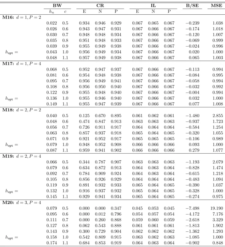
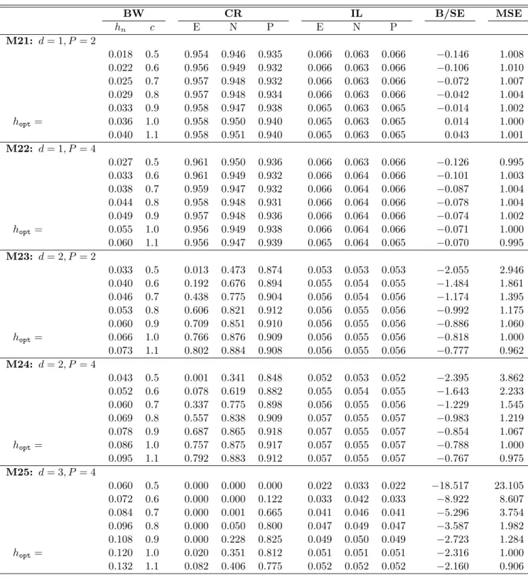
examined, including even the non-differentiable-in-γ example used in the Monte Carlo experiment
of Section 7 (and analyzed in Section SA.3 of the supplemental appendix).
Whereas it is usually most efficient to proceed on a case-by-case basis when verifying the first part of Condition AS, the second part of the condition admits general sufficient conditions that are both mild and relatively simple. A common way of verifying the second part of Condition SE (i.e.,
the stochastic equicontinuity counterpart of Condition AS) is to exhibit a sequence Γn satisfying
P(ˆγn∈Γn)→1 and sup γ∈Γn 1 √ n n X i=1 [ˉg0(zi, γ)−Gˉ0(γ)−gˉ0(zi, γ0) + ˉG0(γ0)] =oP(1),
where empirical process results (e.g., maximal inequalities) can be used to formulate primitive
sufficient conditions for the latter (see, e.g., Andrews (1994b, Condition (3.36)),Chen, Linton, and
van Keilegom(2003, Conditions (2.4) and (2.50)), and references therein). An analogous approach
does not seem applicable when the goal is to formulate primitive sufficient conditions for the second
part of Condition AS, as the dependence of ˆγ(ni) on iimplies that the second part of Condition AS
cannot be deduced with the help of a result of the form sup γ∈Γn 1 √ n n X i=1 [ˉgn(zi, γ)−Gˉn(γ)−ˉgn(zi, γn) + ˉGn(γn)] =oP(1).
Instead, the proof of the following lemma exploits the fact that the object of interest can be
expressed as a linear combination of U-statistics when ˆγn is kernel-based. Here, and else where
in the paper, it is tacitly assumed that the indices i, j, and k are distinct, unless explicitly noted
otherwise.
Lemma 2 Suppose that γˆn is kernel-based, that gˉn is of the form (5), and that V(gn,γ(zi)[ˆγjn−γn]) =o(n), V(gn,γγ(zi)[ˆγjn−γn,ˆγkn−γn]) =o(n2),
V(E(gn,γγ(zi)[ˆγjn−γn,γˆjn−γn]|zi)) =o(n2), V(gn,γγ(zi)[ˆγjn−γn,γˆjn−γn]) =o(n3). Then the second part of Condition AS is satisfied.
5.3 Condition AN
When ˉgnis of the form (5), we have 1 √ n n X i=1 [gn(zi, γn) + ˉGn(ˆγn(i))−Gˉn(γn)] = 1 √ n n X i=1 ψn(zi) +√nBˆn, where ψn(zi) =gn(zi, γn)−Gn(γn) +δn(zi), δn(zi) =Gn,γ[ˆγin−γn], and ˆ Bn=Gn(γn) + 1 2 1 n n X i=1 Gn,γγ[ˆγ(ni)−γn,ˆγ(ni)−γn].
Direct calculations can usually be used to demonstrate existence of a function ψ0 satisfying
Ekψn(z)−ψ0(z)k2 →0, Ekψ0(z)k2<∞. (10)
Indeed, under general conditions, (10) holds with ψ0(z) = g0(z, γ0) +δ0(z), where δ0(z) is the
“correction term” discussed byNewey(1994a). If (10) holds, then Condition AN is satisfied if also
ˆ
Bn=Bn+oP(n−1/2).A simple sufficient condition for this to occur is given in the next result.
Lemma 3 Suppose that γˆn is kernel-based, that gˉn is of the form (5), that (10) holds, and that V(Gn,γγ[ˆγin−γn,γˆin−γn]) =o(n2), V(Gn,γγ[ˆγin−γn,ˆγjn−γn]) =o(n).
Then Condition AN holds with Ω0=V[ψ0(z)] and any Bn=EBˆn+o(n−1/2). 5.4 Conditions AL*, AS*, and AN*
Condition AL* can often be verified with the help of the following bootstrap analogue of Lemma
1.
Lemma 4 Suppose that the assumptions of Lemma 1 are satisfied, that ˆθ∗n−θ0 =oP(1),and that:
(i*) Gˆ∗n(ˆθ∗n,γˆ∗n)0Wˆn∗Gˆ∗n(ˆθ∗n,γˆ∗n)≤infθ∈ΘGˆ∗n(θ,γˆn∗)0Wˆn∗Gˆ∗n(θ,γˆ∗n) +oP(n−1); (ii*) for every δn=o(1),
sup
kθ−θ0k≤δn
kG(θ,ˆγ∗n)−G(θ0,ˆγ∗n)−G˙(ˆγ∗n)(θ−θ0)k
kθ−θ0kρ/2 =oP(1);
(iii*) for every δn=o(1), sup kθ−θ0k≤δn kGˆ∗ n(θ,γˆ∗n)−G(θ,γˆ∗n)−Gˆn∗(θ0,ˆγ∗n) +G(θ0,ˆγ∗n)k 1 +n1/ρkθ−θ0k =oP(n− 1/ρ);
(iv*) Gˆ∗n(θ0,γˆ∗n) =OP(n−1/ρ);
(vi*) Wˆn∗−Wn=oP(n1/ρ−1/2) and G˙(ˆγ∗n)−G˙n=oP(n1/ρ−1/2); (vii*) G˙(ˆγ∗n)0Wˆn∗Gˆ∗n(ˆθ∗n,γˆ∗n) =oP(n−1/2) and, for every δn=O(n−1/ρ),
sup
kθ−θ0k≤δn
kGˆ∗n(θ,γˆ∗n)−G(θ,γˆ∗n)−Gˆ∗n(θ0,ˆγ∗n) +G(θ0,ˆγn∗)k=oP(n−1/2).
Then Condition AL* holds with J∗
n =Jn and J0∗ =J0.
When the first part of Condition AS is satisfied with ˉgn of the form (5), there usually exist
linear and bilinear functionals gn,γ∗ (z)[∙] and g∗n,γγ(z)[∙,∙] such that the first part of Condition AS*
is satisfied with ˉ
gn∗(z, γ) =gn∗(z,γˆn) +gn,γ∗ (z)[γ−ˆγn] +1
2g∗n,γγ(z)[γ−γˆn, γ−ˆγn]. (11)
Conditions under which the second part of Condition AS* holds when ˉg∗n is of the form (11) are
given in the following bootstrap analogue of Lemma 2.
Lemma 5 Suppose that γˆ∗n is kernel-based, that gˉn∗ is of the form (11), and that V∗(g∗
n,γ(zi,n∗ )[ˆγ∗n,j−γˆn]) =oP(n), V∗(gn,γγ∗ (zi,n∗ )[ˆγ∗n,j−ˆγn,ˆγn∗,k−ˆγn]) =oP(n2), V∗(E∗(g∗
n,γγ(zi,n∗ )[ˆγn∗,j−ˆγn,ˆγn∗,j−γˆn]|zi,n∗ )) =oP(n2), V∗(gn,γγ∗ (z∗i,n)[ˆγ∗n,j−γˆn,ˆγ∗n,j−γˆn]) =oP(n3), where V∗[∙] denotes V[∙|z1, . . . , zn].Then the second part of Condition AS* is satisfied.
Finally, when ˉg∗n is of the form (11), we have
1 √ n n X i=1 [g∗n(zi,n∗ ,γˆn) + ˉG∗n(ˆγn∗,(i))−Gˉ∗n(ˆγn)] = √1 n n X i=1 ψ∗n(zi,n∗ ) +√nBˆn∗, where
ψ∗n(zi,n∗ ) =gn∗(zi,n∗ ,γˆn)−G∗n(ˆγn) +δ∗n(z∗i,n), δ∗n(z∗i,n) =G∗n,γ[ˆγ∗n,i−γˆn],
and ˆ B∗n=G∗n(ˆγn) + 1 2 1 n n X i=1 G∗n,γγ[ˆγ∗n,(i)−ˆγn,ˆγ∗n,(i)−ˆγn], with
Gn∗(γ) =E∗gn∗(zi,n∗ , γ), G∗n,γ[η] =E∗gn,γ∗ (zi,n∗ )[η], G∗n,γγ[η, ϕ] =E∗g∗n,γγ(zi,n∗ )[η, ϕ].
Direct calculations can usually be used to show that E∗kψ∗
in which case the following bootstrap analogue of Lemma 3can be used to verify Condition AN*.
Lemma 6 Suppose that the assumptions of Lemma 3 are satisfied, thatγˆ∗nis kernel-based, that ˉg∗n is of the form (11), that (12) holds, and that
V∗(G∗
n,γγ[ˆγ∗n,i−ˆγn,ˆγn∗,i−γˆn]) =oP(n2), V∗(G∗n,γγ[ˆγ∗n,i−γˆn,γˆ∗n,j−γˆn]) =oP(n), E∗Bˆ∗
n=EBˆ∗n+oP(n−1/2). Then Condition AN* holds with Ω∗
0 = Ω0 and any B∗n=EBˆn∗ +o(n−1/2).
Remark 3 If the conditions of Lemma 6 are satisfied, then Ωˆn = n−1Pni=1ψ∗n(zi)ψ∗n(zi)0 is a consistent estimator ofΩ0.AlthoughΩnˆ emerges here as a by-product of our analysis of the bootstrap
it is interesting to note that it can be interpreted as a variant of the “delta-method” variance estimator of Newey (1994b).
6
Example: Inverse Probability Weighting
In the previous sections, the average density example was chosen for illustrative purposes because it highlights exactly those parts of our high-level assumptions that differ from conventional ones, namely Condition AN (which quantifies the departure from conventional conclusions) and the second part of Condition AS (which enables us to depart from conventional assumptions). Indeed, the estimators discussed in connection with Example 1 were intentionally chosen in such a way that Condition AL and the first part of Condition AS are representations in the sense that they hold without any oP(n−1/2) andoP(1) terms.
To substantiate the claim that Example 1 is nevertheless representative, this section examines a more substantive and complicated class of estimators, namely IPW estimators. For these estimators, Condition AL and the first part of Condition AS are not merely representations, but as discussed in what follows they nevertheless remain verifiable under assumptions that are sufficiently weak to permit us to obtain distributional results that differ from conventional ones, a difference that once again is quantified by Condition AN and can be brought to light thanks to the second part of Conditions AS.
Supposez1, . . . , zn arei.i.d. copies ofz= (y, t, x0)0,wherey∈R is a scalar dependent variable,
t∈ {0,1}is a binary indicator, and x∈X⊆Rdis a continuous covariate with densityf
0.Assuming
the estimandθ0 ∈Θ⊆Rdθ is the unique solution to an equation of the form
E t q0(x) m(y;θ) = 0, q0(x) =E(t|x) =P[t= 1|x],
wherem is a known Rdθ-valued function, an IPW estimator ˆθ
n of θ0 is one that satisfies
1 n n X i=1 ti ˆ qn(xi)m(yi; ˆθn) =oP(n −1/2),
where ˆqn is an estimator of (the propensity score) q0.
In what follows we assume that q0 is estimated using a local polynomial estimator of order
P >3d/4−1.To describe this estimator, define dP = (P+d−1)!/[P!(d−1)!],and letbP(x)∈RdP denote the P-th order polynomial basis expansion based on x= (x1, . . . , xd)0 ∈Rd; that is,
bP(x) = 1 [x]1 ... [x]P , [x] p = xp1 xp1−1x2 ... xpd . Also, let ˆ γx,n(x) = vecP[1 n n X i=1 Kx,n(xi−x)], Kx,n(u) =bP,n(u)bP,n(u)0Kn(u), and ˆ γt,n(x) = 1 n n X i=1 tiKt,n(xi−x), Kt,n(u) =bP,n(u)Kn(u),
where bP,n(u) = bP(u/hn), Kn(u) = K(u/hn)/hdn, hn is a bandwidth, K is a kernel, and where
vecP :RdP×dP → Rd2P is the vectorization operator. The Pth order local polynomial estimator of
q0(x) is given by q(x; ˆγn),where
q(x;γ) =e0P(vec−P1[γx(x)])−1γt(x), γ = (γ0x, γ0t)0, eP is the first unit vector in RdP,and vec−P1:Rd
2
P →RdP×dP is the inverse of vecP.
Because ˆγn is kernel-based, the associated IPW estimator ˆθn is a kernel-based two-step
semi-parametric, which can be analyzed using the results of the previous sections by representing the defining property of ˆθnas ˆ Gn(ˆθn,ˆγn)0WˆnGˆn(ˆθn,γˆn) =oP(n−1), Wˆn=Idθ, where g(z, θ, γ) = t q(x;γ)m(y;θ)
is neither linear in γ nor (necessarily) differentiable in θ. Doing so, it is shown in Section A.2
of the supplemental appendix that under regularity conditions and if nh3nd/2/(logn)3/2 → ∞ and
nh2P+2
n → 0, then the conditions of Theorems 1 and 2 are satisfied. In what follows, we briefly