Contents lists available atScienceDirect
Food Quality and Preference
journal homepage:www.elsevier.com/locate/foodqualReconsidering the classification of sweet taste liker phenotypes:
A methodological review
Vasiliki Iatridi
a,⁎, John E. Hayes
b,c, Martin R. Yeomans
aaSchool of Psychology, University of Sussex, Falmer BN1 9QH, United Kingdom
bDepartment of Food Science, College of Agricultural Sciences, The Pennsylvania State University, PA 16802, United States
cSensory Evaluation Center, College of Agricultural Sciences, The Pennsylvania State University, PA 16802, United States
A R T I C L E I N F O Keywords: Flavor perception Gustation Hedonics Sugar Sweet tooth Taste preference A B S T R A C T
Human ingestive behavior depends on myriad factors, including both sensory and non-sensory determinants. Of the sensory determinants, sweet taste is a powerful stimulus and liking for sweetness is widely accepted as an innate human trait. However, the universality of sweet-liking has been challenged. Sub-groups exhibiting strong liking (sweet likers) or having aversive responses to sweet taste (sweet dislikers) have been described, but the methods defining these phenotypes are varied and inconsistent across studies. Here, we explore the strengths and weaknesses of different methodological approaches in identifying sweet taste liker phenotypes in a compre-hensive review. Prior studies (N= 71) using aqueous sucrose solution-based taste tests and a definition of two or more distinct hedonic responses reported between 1970 and 2017 were summarized. Broadly speaking, four different phenotyping methods have been used: 1. Interpretation (visual or statistical) of the shape of hedonic response curves, 2. Highest preference using ratings, 3. Average liking above mid-point or Positive/Negative average liking method, and 4. Highest preference via paired comparisons. Key methodological weaknesses in-cluded the use of subjective or arbitrary criteria as well as adoption of protocols unsuitable for large-scale implementation. Overall, we did not identify a method distinctly superior to the others. Given the role of both hedonics and reward in food intake, a better understanding of individual variations in sweet taste perception could clarify how sweet-liking interplays with obesity or addictive behaviors such as alcohol misuse and abuse. The development of a universally used statistically robust and less time-consuming classification method is needed.
1. Introduction
Poor food choices and overeating are key contributors to the etiology of many modern chronic diseases, mainly by influencing the development of obesity and obesity-related conditions such as type II diabetes (Darnton-Hill, Nishida, & James, 2004; Swinburn et al., 2011). Human ingestive behavior involves a complex interaction between sensory and non-sensory factors. Biologically determined factors (taste, hunger/fullness mechanisms, sensory-specific satiety), experience/ memory with food (physiological and social conditioning), person-re-lated characteristics (perceptions, beliefs, values, knowledge, family and social networks etc.), and social and environmental determinants (cultural and religious norms; food availability, economic environment, public policies, media etc.) operate together and formulate discrete food choice patterns (Contento, 2016; Drewnowski, 1997; McCrickerd
& Forde, 2016). Of the sensory determinants of food choice, sweet taste is widely accepted as a powerful stimulus that generally signals plea-sure (Drewnowski, Mennella, Johnson, & Bellisle, 2012). According to the delay discounting theory (reviewed inOdum, 2011), this attribute of sweetness could presumably serve as an additional driver of food choice when immediate rewards (e.g. pleasure) are optimized over long-term benefits (e.g. health). Evidence from animal studies and human neuroimaging experiments suggest common neural pathways between addictive substances such as drugs and alcohol and sweet foods and beverages (Alonso-Alonso et al., 2015; Stice, Figlewicz, Gosnell, Levine, & Pratt, 2013), further supporting this key role for sweetness in food acceptance.
The pleasure derived from tasting sweet substances has been con-sidered as an innate response evidenced by the positive facial reactions of newborns from a variety of species to the experience of sweet tastes
https://doi.org/10.1016/j.foodqual.2018.09.001
Received 13 July 2018; Received in revised form 31 August 2018; Accepted 3 September 2018
Abbreviations:BMI, body mass index; gLMS, generalized labeled magnitude scale; HCA, hierarchical cluster analysis; s.d., standard deviation; SD, sweet dislike; SL,
sweet liker; STT, sweet taste test; VAS, visual analog scale ⁎Corresponding author.
E-mail addresses:[email protected](V. Iatridi),[email protected](J.E. Hayes),[email protected](M.R. Yeomans).
Food Quality and Preference 72 (2019) 56–76
Available online 05 September 2018
0950-3293/ © 2018 The Authors. Published by Elsevier Ltd. This is an open access article under the CC BY license (http://creativecommons.org/licenses/BY/4.0/).
Table 1 Papers included in this review using the ‘Visual discrimination of hedonic responses’ classification method (Method 1a) for the identification of the distinct sweet taste liker phenotypes. Author(s), Publication Year Country Participants n (% men) Health Status (%) Age in years mean (± s.d.) * Sucrose Solutions (× times of replicates) Hedonic Scale Sweet taste liker phenotypes (%) Oleson and Murphy (2017) USA 40 (50) Healthy (100) 19.0 (1.6) 0.058, 0.12, 0.23, 0.47, and 0.93 M §(× 2) gLMS – High concentration liker (47.5): ↑SUC = > ↑LIKE – Moderate concentration liker (52.5): ↑SUC = > ↓LIKE or ↑↓LIKE ,breakpoint at 0.23 M Eikemo et al. (2016) Norway 49 (100) Healthy (100) 24.7 (3.9) 0.05, 0.10, 0.20, 0.42, and 0.65 M (× 3) VAS – SL (46.9): ↑SUC = > ↑LIKE – SD (53.1): ↑SUC = > ↓LIKE Thai et al. (2011) 1 Malaysia 325 (49) Healthy (100) 21.0 (14.5) 0.087, 0.22, and 0.55 M §(x 1) gLMS – Type II (48.9): ↑SUC = > ↑→ LIKE – Type I(51.1): ↑SUC = > ↑↓LIKE ,breakpoint at 0.22 M Yeomans et al. (2007) (see also Table 4 ) UK 60 (33) Healthy (100) 23.1 (6.2 †) 0.05, 0.21, 0.42, and 0.83 M (× 2) VAS – SL (66.7): ↑SUC = > ↑LIKE – SD (33.3): ↑SUC = > ↓LIKE or ↑↓LIKE ,breakpoint at 0.21 M Holt et al. (2000) Australia 132 (42) Healthy (100) Australian: 22.8 (4.3) Malaysian: 21.5 (1.2) 0.058, 0.12, 0.23, 0.47, and 0.93 M §(× 1) 3-point scale – SL (12.1): ↑SUC = > ↑LIKE – SD (87.9): ↑SUC = > ↓LIKE or ↑↓LIKE ,breakpoints at 0.12 or 0.23 M Drewnowski et al. (1998) 2 USA 121 (0) Healthy (100) 27.7 ( **) 0.058, 0.12, 0.23, 0.47, and 0.93 M (× **) 9-point category scale – SL (41.3): ↑SUC = > ↑LIKE – SD (52.1): ↑SUC = > ↓LIKE + 8 participants with undefined sweet taste liker phenotype Drewnowski, Henderson, Shore, and Barratt-Fornell (1997) USA 159 (0) Healthy (100) 27.0 (8.8 ††) 0.058, 0.12, 0.23, 0.47, and 0.93 M (× 1) 9-point category scale – SL (41.5): ↑SUC = > ↑→ LIKE – SD (51.6): ↑SUC = > ↓LIKE or ↑↓LIKE ,breakpoint at ** + 11 participants with undefined sweet taste liker phenotype Drewnowski, Henderson, and Shore (1997) USA 87 (0) Healthy (100) 25.4 (5.6 ††) 0.058, 0.12, 0.23, 0.47, and 0.93 M (× 1) 9-point category scale – SL (34.5): ↑SUC = > ↑→ LIKE – SD (65.5): ↑SUC = > ↓LIKE Franko et al. (1994) USA 40 (0) Bulimia nervosa (38) Bulimia nervosa with history of anorexia (12) Bulimia nervosa: 25.0 (4.0) 0.039, 0.078, 0.149, 0.30, 0.632, and 1.632 M ‡‡(× 2) analogue scale – (37.5): ↑SUC = > ↑→ LIKE – (50.0): ↑SUC = > ↑↓LIKE ,breakpoint at 0.078 M – (12.5): ↑SUC = > ↓LIKE Healthy (50) Controls: 24.0 (4.0) Travers et al. (1993) USA 41 (61) PD (61) PD patients M: 62.4 (5.0) F: 67.8 (8.3) 0.04 3,0.08, 0.15, 0.3, 0.6, 0.9, and 1.5 M (× 1) 6-point category scale – (36.6): ↑SUC = > ↑→ LIKE – (63.4): ↑SUC = > ↑↓LIKE ,breakpoint at 0.3 M Healthy (39) Controls: M: 64.4 (7.8) F: 61.2 (3.8) Looy et al. (1992) Canada Group 1: 22 (41) **( **) **( **) 0.05, 0.10, 0.21, 0.42, and 0.83 M (× 5) VAS Group 1 – SL (40.1): ↑SUC = > ↑LIKE – SD (31.8): ↑SUC = > ↓LIKE + 6 participants with neutral, inverted U-shaped or erratic response Group 2: 38 (29) **( **) **( **) Group 2 – SL (34.2): ↑SUC = > ↑LIKE – SD (36.8): ↑SUC = > ↓LIKE + 11 participants with neutral, inverted U-shaped or erratic response Looy & Weingarten (1992) Canada 66 (42) **( **) 20.3 (3.5) VAS – SL (33.3): ↑SUC = > ↑LIKE ( continued on next page )
Table 1 ( continued ) Author(s), Publication Year Country Participants n (% men) Health Status (%) Age in years mean (± s.d.) * Sucrose Solutions (× times of replicates) Hedonic Scale Sweet taste liker phenotypes (%) 0.05, 0.10, 0.21, 0.42, and 0.83 M (× 8) – SD (50): ↑SUC = > ↓LIKE – Neutral (10.6):↑ SUC = > →LIKE + 4 participants with erratic response Looy & Weingarten (1991) Canada 28 (43) **( **) 20.5 (3.5) 0.03, 0.05, 0.10, 0.16, 0.21, 0.31, 0.42, 0.62, and 0.83 M (× 8) VAS – SL (32.2): ↑SUC = > ↑LIKE – SD (46.4): ↑SUC = > ↓LIKE – Neutral (21.4):↑ SUC = > →LIKE Drewnowski & Schwartz (1990) USA 50 (0) Healthy (100) 20.2 (1.7) 0.059, 0.24, 0.50, and 1.06 M §§ (× 1) 9-point category scale – Type II 4(36.0): ↑SUC = > ↑LIKE – Type I 4(64.0): ↑SUC = > ↓LIKE or ↑↓LIKE ,breakpoint at 0.24 M Frijters and Rasmussen-Conrad (1982) NL 25 (0) Overweight (51) Normal weight (48) [24–53 years old] 0.06, 0.1148, 0.2089, 0.3082, 0.6918, and 1.3 M (× 3) 3-anchor line (midpoint for the ideal sweetness) – Type II (4.0): ↑SUC = > ↑LIKE – Type I(92.0): ↑SUC = > ↑↓LIKE ,breakpoint at ** – Neutral (4.0): ↑SUC = > →LIKE Malcolm et al. (1980) USA 22 (0) Healthy (100) [18–40 years old] 0.006 5,0.012 5,0.03 5,0.06 5, 0.09, 0.15, 0.3, 0.5, 0.8 and 1 M (1 ×) 9-point category scale – Type II (45.5): ↑SUC = > ↑→ LIKE – Type I(54.5): ↑SUC = > ↑↓LIKE ,breakpoints at 0.3 M and 0.5 M Johnson et al. (1979) USA 49 ( **) Obese in weight loss (65) Behavior modification weight loss:36.0 ( **) Meal replacement weight loss: 35.0 ( **) 0.058, 0.10, 0.17, 0.32, 0.58, and 1.46 M §(× 2) 9-point category scale – Type II (30.6): ↑SUC = > ↑LIKE – Type I(69.4): ↑SUC = > ↑↓LIKE ,breakpoints at 0.17 and 0.32 M Normal weight (35) Controls: 24.0 ( **) Enns et al. (1979) USA Children: 21 (76) **( **) Children M:10.5 (0.2 ††) W: 10.7 (0.3 ††) 0.056, 0.1, 0.17, 0.32, 0.56, and 1.0 M (× 3) 9-point category scale Children: – (76.2): ↑SUC = > ↑LIKE – (23.8): ↑SUC = > ↓LIKE Young adults: 27 (63) **( **) Young adults M: 19.0 (1.0 ††) W: 18.3 (1.6 ††) Young adults: – (63.0): ↑SUC = > ↑LIKE – (37.0): ↑SUC = > ↑↓LIKE ,breakpoint at 0.32 M Elderly: 12 (42) **( **) Elderly M:71.6 (2.8 ††) W: 70.5 (3.6 ††) Elderly: – (41.7): ↑SUC = > ↑LIKE – (58.3): ↑SUC = > ↓LIKE Grinker (1977) 6(see also Table 5 ) USA 56 (34) Extremely obese (45) Extremely obese: 34.2 ( **) 0.057, 0.10, 0.17, 0.32, and 0.57 M §(× 1) 9-point category scale – (30.4): ↑SUC = > ↑→ LIKE – (69.6): ↑SUC = > ↓LIKE Moderately obese (25) Moderately obese: 32.7 ( **) Normal weight (30) Normal weight: 23.1 ( **) Thompson et al. (1977) USA 32 ( **) Obese (44) Normal weight (56) 20.0 (3.0) 0.075, 0.15, 0.3, 0.6, 0.9, 1.2, and 1.5 M (× 1) Magnitude estimation method – Type II (31.2): ↑SUC = > ↑LIKE – Type I(68.8): ↑SUC = > ↑↓LIKE ,breakpoint at 0.6 M Thompson et al. (1976) USA Group 1 18 (61) Normal weight (100) Group 1 Type II: 19.6 (1.5) Type I: 19.2 (1.3) Group 1 0.075, 0.15, 0.3, 0.6, 0.9, 1.2, and 1.5 M Magnitude estimation method Group 1 – Type II (27.8): ↑SUC = > ↑→ LIKE – Type I(72.2): ↑SUC = > ↑↓LIKE ,breakpoint at 0.3 M ‡ Group 2 59 (19) Overweight/Obese (100) Group 2 Type II: 33.9 (15.9) Type I: 38.3 (13.4) Group 2 0.06, 0.1, 0.25, 0.4, 0.7, 1.0, and 2.0 M (× 1) Group 2 – Type II (35.6): ↑SUC = > ↑→ LIKE – Type I(64.4): ↑SUC = > (↑)↓ LIKE ,breakpoint at 0.25 M ‡ Grinker & Hirsch (1972) 7,8 USA 23 ( **) **( **) 7-point category scale ( continued on next page )
Table 1 ( continued ) Author(s), Publication Year Country Participants n (% men) Health Status (%) Age in years mean (± s.d.) * Sucrose Solutions (× times of replicates) Hedonic Scale Sweet taste liker phenotypes (%) Obese (43) Normal weight (57) 0.057, 0.10, 0.18, 0.33, and 0.61 M §§(× 1) – (56.5): ↑SUC = > ↑↓LIKE with breakpoint at 0.18 M – (43.5): ↑SUC = > ↓LIKE Pangborn (1970) USA 29 (1 0 0) 8 **( **) **( **) 0.023, 0.059, 0.094, 0.13, 0.17, 0.20, and 0.24 M §§‡ (× 5) 9-point category scale – Like (55.0): ↑SUC = > ↑LIKE – Like-dislike (20.0): ↑SUC = > ↑↓LIKE ,breakpoint at 0.094 M – Dislike (25.0): ↑SUC = > 1↓LIKE Notes: *Age mean and s.d. rounded to one decimal place. **No information available. †s.d. calculated from standard error (SE) (SE = s.d./√sample size). ††s.d. calculated from standard error of the mean (SEM) (SEM = s.d./√sample size). §Sucrose concentration in M (mol/L) calculated from % w/v based on sucrose’s molecular weight (342.296 g) and the assumption that the solvent is pure/deionized water at 20 °C ( Haynes, 2016 ). §§Sucrose concentration in M (mol/L) calculated from % w/w based on sucrose’s molecular weight (342.296 g) and the assumption that the solvent is pure/deionized water at 20 °C (% w/w = % w/v × Special Gravity solution )( Haynes, 2016 ). ‡Based on reviewers’ conclusion after interpreting the shape of the hedonic response curves. ‡‡Based on reviewers’ assumption that the sucrose concentration was initially expressed in % w/w. 1The between-sex sweet taste liker phenotypes results are presented. 2It is not clear whether there is an overlap between participants in the current report ( Drewnowski et al., 1998 )and those in Drewnowski, Henderson, Shore, and Barratt-Fornell (1997) . 3Only 28 of the 41 participants tasted and rated the 0.04 M solution. 4Type Iand II sweet taste liker phenotypes’ description is adjusted based on Thompson and colleagues original paper ( Thompson, et al., 1976 ). 5The relevant liking ratings weren’t included in the sweet taste liker phenotype classification. 6It is not clear whether the presented sweet taste liker phenotypes results being were collected before or after the red “cherry” colour manipulation of the sucrose solutions. 7Original reference in Grinker, J., Smith, D. V. & Hirsch, J. (1971) .Taste preferences in obese and normal weight subjects. Proceedings of the IVth International Conference on the Regulation of Food and Water Intake , Cambridge, England (abstract). 8It is not clear whether there is an overlap between participants rating stimuli on a hedonic scale ( Table 1 )or those tested via the paired-comparison technique ( Table 5 ). 9Only 20 of the 29 participants completed the entire series of replicates. ↑SUC :Increasing sucrose concentration. ↓LIKE :Descending liking rating. ↑↓LIKE :Inverted U-shaped hedonic response curve. ↑LIKE :Ascending liking rating. ↑→ LIKE :Ascending liking rating followed by a plateau. →LIKE :Consistent liking rating. AN, anorexia nervosa; BMI, body mass index; gLMS, generalized Labeled Magnitude Scale; liking ratingM, men; NL, The Netherlands; PD, Parkinson disease; SUC, sucrose concentration; s.d., standard deviation; SD, sweet disliker; SL, sweet liker; VAS, Visual Analog Scale; W, women .
Table 2 Papers included in this review using the ‘Statistical discrimination of hedonic responses’ classification method (algorithmic classification: Method 1b) for the identification of the distinct sweet taste liker phenotypes. Author(s), Publication Year Country Participants n (% men) Health Status (%) Age in years mean (± s.d.) * Sucrose Solutions (× times of replicates) Hedonic Scale Sweet taste liker phenotypes (%) Garneau et al. (2018) 1 USA Children: 303 (41) Healthy ( **) Unhealthy ( **) Children: 10.9 (2.2) 0.070, 0.13, 0.22, and 0.40 M §(× 1) VAS Children – Cluster 1 – SL (78.2): ↑SUC = > ↑LIKE – Cluster 2 – SD (21.8): ↑SUC = > ↓LIKE Adults: 650 (38 †) Healthy ( **) Unhealthy ( **) Adults: 41.8 (16.5) Adults – Cluster 1 – SL (33.5): ↑SUC = > ↑LIKE – Cluster 2 – Neutrals (17.7 + 40.3): ↑SUC = > ↑↓LIKE , breakpoint at **and = > →LIKE – Cluster 3 – SD (8.5): ↑SUC = > ↓LIKE Kim et al. (2017) Republic of Korea 120 (0) **( **) 24 ( **) 0.087, 0.17, 0.35, 0.70, and 1.05 M §(× 1) 9-point category scale – Cluster 4 + 5 – SL (32.5): ↑SUC = > ↑LIKE – Cluster 1 (35.8): ↑SUC = > ↑↓LIKE ,breakpoint at 0.35 M – Cluster 2 + 3 – SD (31.7): ↑SUC = > ↓LIKE Methven et al. (2016) (see also Table 4 ) UK 36 (34 2) **( **) 26 ( **) 0.087, 0.17, 0.35, 0.70, and 1.05 M §(× 1) VAS – Cluster 1 – SL (36.1):↑ SUC = > ↑LIKE – Cluster 2 – SD (63.9): ↑SUC = > ↑↓LIKE ,breakpoint at 0.17 M Asao et al. (2015) (see also Table 5 ) USA 26 (46) Healthy (100) 32.6 (14.5) 0.035, 0.053, 0.079, 0.118, 0.177, 0.266, 0.399, 0.598, 0.897, and 1.346 M (× 2) VAS – Cluster 2 – High concentration liker (50.0): ↑SUC = > ↑LIKE – Cluster 1 – Low concentration liker (50.0): ↑SUC = > ↑ ↓LIKE ,breakpoints between 0.118 M and 0.266 M Kim et al. (2014) Republic of Korea 200 (0) **( **) 22 ( **) 0.087, 0.17, 0.35, 0.70, and 1.05 M §(× 1) VAS – Cluster 1 (49.5): ↑SUC = > ↑LIKE – Cluster 2 (31.5): ↑SUC = > ↑↓LIKE ,breakpoint at 0.70 M or ≈ > ↑→ LIKE – Cluster 3 (19.0): ↑SUC = > ↑↓LIKE ,breakpoint at 0.35 M Notes *Age mean and s.d. rounded to one decimal place. **No information available. §Sucrose concentration in M (mol/L) calculated from % w/v based on sucrose’s molecular weight (342.296 g) and the assumption that the solvent is pure/deionized water at 20 °C ( Haynes, 2016 ). 1The paper was available online on the 12th of October 2017. 2One participant denied the relevant information. ↑SC :Increasing sucrose concentration. ↓LIKE :Descending liking rating. ↑↓LIKE :Inverted U-shaped hedonic response curve. ↑LIKE :Ascending liking rating. →LIKE :Consistent liking rating. BMI, body mass index; gLMS, general labeled magnitude scale; LIKE, liking rating; SUC, sucrose concentration; s.d., standard deviation; SD, sweet disliker; SL, sweet liker; VAS, visual analog scale.
Table 3 Papers included in this review using the ‘Highest preference using ratings’ classification method (Method 2) for the identification of the distinct sweet taste liker phenotypes. Author(s), Publication Year Country Participants n (% men) Health Status (%) Age in years mean (± s.d.) * Sucrose Solutions (× times of replicates) Hedonic Scale Sweet taste liker phenotypes (%) Eiler et al. (2018) 1 USA 74 (43) Healthy (100) 22.8 (1.6) 0.05, 0.10, 0.21, 0.42, and 0.83 M (× 3) ** – SL (35.1): LIKE max at 0.83 M – SD (63.5): LIKE max at 0.05, 0.10, 0.21, or 0.42 M + 1 participant with no available data Goodman et al. (2018) 2 USA 41 (15) Binge-eating disorder (100) 38.0 (11.5) 0.05, 0.10, 0.21, 0.42, and 0.83 M (× 5) analogue scale – Highest sweet preferer (43.9): LIKE max at 0.83 M – Other sweet preferer (56.1): LIKE max at 0.05, 0.10, 0.21, or 0.42 M Weafer et al. (2017) USA 71 (51 3) Healthy (100) [21–35 years old] 0.05, 0.10, 0.21, 0.42, and 0.83 M (× 5) VAS – SL (50.7): LIKE max at 0.83 M – SD (47.9): LIKE max at 0.05, 0.10, 0.21, or 0.42 M + 1 participant with non-appropriate concentration–response curve Turner-McGrievy et al. (2016) USA 209 (16) Obese in weight loss (100) 42.3 (11.0) 0.05, 0.10, 0.21, 0.42, and 0.83 M (× 5) VAS – SL (33.5): LIKE max at 0.83 M – SD (66.5): LIKE max at 0.05, 0.10, 0.21, or 0.42 M Garbutt et al. (2016) USA 80 (71) Alcoholic (100) 47.0 (8.6) 0.05, 0.10, 0.21, 0.42, and 0.83 M (× 5) analogue scale – SL (27.5): LIKE max at 0.83 M – SD (72.5): LIKE max at 0.05, 0.10, 0.21, or 0.42 M Swiecicki et al. (2015) Poland 72 (29) Depressed with SAD (25) Depressed with SAD: 36.3 (9.3 †) 0.029, 0.30, and 0.99 M §§(× 2) 2-anchor line – SL (71.0): LIKE max at 0.99 M – SD (29.0 ‡): LIKE max at 0.029 or 0.30 M Depressed without SAD (33) Depressed without SAD: 36.8 (10.3 †) Healthy (42) Controls: 35.4 (11.5 †) Weafer, Burkhardt, and de Wit (2014) USA 20 ( **) Healthy (100) [18–30 years old] 0.05, 0.10, 0.21, 0.42, and 0.83 M (× 5) VAS – SL ( **): LIKE max at 0.83 M – SD ( **): LIKE max at 0.05, 0.10, 0.21, or 0.42 M + 1 participant with non-appropriate concentration–response curve Kampov-Polevoy et al. (2014) USA 150 (49) Alcohol use disorders+ (50) Alcohol use disorders− (50) 21.0 (1.8) 0.05, 0.10, 0.21, 0.42, and 0.83 M (× 5) VAS – SL (50.0): LIKE max at 0.83 M – SD (50.0): LIKE max at 0.05, 0.10, 0.21, or 0.42 M Damiano et al. (2014) USA 57 (88) ASD (33) Healthy (67) ASD patients: 26.0 (8.0) Controls: 20.4 (5.6) 0.05, 0.10, 0.21, 0.42, and 0.83 M (× 5) analogue scale – SL (49.1): LIKE max at 0.83 M – SD (50.9): LIKE max at 0.05, 0.10, 0.21, or 0.42 M Kareken et al. (2013) USA 16 (75) Healthy (100) 26.1 (4.4) 0.05, 0.10, 0.21, 0.42, and 0.83 M (× 3) VAS – SL (50.0): LIKE max at 0.83 M – SD (50.0): LIKE max at 0.05, 0.10, 0.21, or 0.42 M Sienkiewicz-Jarosz et al. (2013) Poland 40 (38) PD (50) Healthy (50) PD patients: 60.6 (27.7 ††) Controls: 56.3 (7.2 ††) 0.029, 0.30, and 0.99 M §§(× 2) 2-anchor line – SL (70.0): LIKE max at 0.99 M – SD (30.0 ‡): LIKE max at 0.029 or 0.30 M Turner-McGrievy et al. (2013) USA 196 (16) Overweight/Obese (100) 42.6 (11.0) 0.05, 0.10, 0.21, 0.42, and 0.83 M (× 5) analogue scale – SL (35.2): LIKE max at 0.83 M – non-SL (64.8 ‡): ** Langleben et al. (2012) USA 15 (87) Opioid-dependent (100) 34.3 (8.2) 0.05, 0.10, 0.21, 0.42, and 0.83 M (× 3) Likert scale – SL (33.3): LIKE max at 0.83 M – SD (66.7): LIKE max at 0.05, 0.10, 0.21, or 0.42 M Dichter et al. (2010) ‡‡ USA 31 ( **) Depressed (52) Healthy (48) Depressed: **( **) Controls: **( **) 0.05, 0.10, 0.21, 0.42, and 0.83 M (× 5) analogue scale – SL (12.9): LIKE max at 0.83 M – SD (87.1‡): LIKE max at 0.05, 0.10, 0.21, or 0.42 M Lange et al. (2010) USA 158 (39) Healthy 4with FHA+ (50) Healthy 4with FHA− (50) [20–25 years old] 0.05, 0.10, 0.21, 0.42, and 0.83 M (× 5) analogue scale – SL (55.1): LIKE max at 0.83 M – SD (44.9 ‡): LIKE max at 0.05, 0.10, 0.21, or 0.42 M ( continued on next page )
Table 3 ( continued ) Author(s), Publication Year Country Participants n (% men) Health Status (%) Age in years mean (± s.d.) * Sucrose Solutions (× times of replicates) Hedonic Scale Sweet taste liker phenotypes (%) Tremblay et al. (2009) USA 215 (55) Alcoholic (43) Healthy (57) Alcoholics: 47.7 (9.1) Controls: 25.9 (6.0) 0.05, 0.10, 0.21, 0.42, and 0.83 M (× 5) VAS – SL (40.5): LIKE max at 0.83 M – SD (14.0): LIKE max at 0.05 M + 85 participants with LIKE max at 0.10, 0.21, or 0.42 M + 13 participants with no preference Swiecicki et al. (2009) Poland 76 (32) Depressed (61) Healthy (39) Depressed: 38.2 (10.9 †)Controls: 35.4 (11.5 †) 0.029, 0.30, and 0.99 M §§(× 2) 2-anchor line – SL (63.2): LIKE max at 0.99 M – SD (36.8 ‡): LIKE max at 0.029 or 0.30 M Garbutt et al. (2009) USA 40 (73) Alcoholic (100) 49.0 (9.0) 0.05, 0.10, 0.21, 0.42, and 0.83 M(x 5) analogue scale – SL (37.5): LIKE max at 0.83 M – SD (62.5): LIKE max at 0.05, 0.10, 0.21, or 0.42 M Wronski et al. (2006) Poland 78 (100) Alcoholic (58) Healthy (42) Alcoholics: 44.3 (10.1 ††) Controls: 42.8 (11.5 ††) 0.029, 0.30, and 0.99 M §§(× 2) 2-anchor line – SL (60.3): LIKE max at 0.99 M – SD ( **): ** Kampov-Polevoy et al. (2006) USA 163 (39) Healthy (100) 22.1 (2.6 ††) 0.05, 0.10, 0.21, 0.42, and 0.83 M (× 5) analogue scale – SL (52.8): LIKE max at 0.83 M – SD (46.0): LIKE max at 0.05, 0.10, 0.21, or 0.42 M + 2 participants with no available data Krahn et al. (2006) ‡‡ USA 65 (100) Alcoholic (100) [18–65 years old] 0.05, 0.10, 0.21, 0.42, and 0.83 M (× 5) VAS – SL (56.9): LIKEmax at 0.83 M – SD ( **): ** Kampov-Polevoy et al. (2004) 5 USA 165 (49) Alcohol or drug abuse disorder and/or psychiatric disorder (100) 37.7 (11.6 ††) 0.05, 0.10, 0.21, 0.42, and 0.83 M (× 5) analogue scale – SL (31.5): LIKE max at 0.83 M – SD (68.5 ‡): LIKE max at 0.05, 0.10, 0.21, or 0.42 M Kampov-Polevoy, Garbutt et al. (2003) USA 163 (39) Healthy with PHA+ (50) Healthy with PHA-(50) 22.1 (2.6 ††) 0.05, 0.10, 0.21, 0.42, and 0.83 M (× 5) analogue scale – SL (50.9): LIKE max at 0.83 M – SD (49.1 ‡): LIKE max at 0.05, 0.10, 0.21, or 0.42 M Kampov-Polevoy et al. (2003) USA 180 (48) Alcohol or drug abuse disorder and/or psychiatric disorder (100) 37.7 (12.1 ††) 0.05, 0.10, 0.21, 0.42, and 0.83 M (× 5) analogue scale – SL (31.0 6): LIKE max at 0.83 M – SD (69.0 6): LIKE max at 0.05, 0.10, 0.21, or 0.42 M Janowsky et al. (2003) USA 32 (34) Cocaine dependent (50) Depressed (50) Cocaine dependent: 34.6 (6.6) Depressed: 31.7 (9.4) 0.05, 0.10, 0.21, 0.42, and 0.83 M (× 5) 10-point analogue scale – SL (28.1): LIKEmax at 0.83 M – SD ( **): ** + 1 participant with LIKE max at both 0.42 and 0.83 M Bogucka-Bonikowska et al. (2002) Poland 60 (100) Opioid-dependent (47) Healthy (53) Opioid-dependent: 40.5 (5.9) Controls: 41.3 (9.0) 0.029, 0.29, and 0.87 M § (× 1) 2-anchor line – SL (50.0): LIKE max at 0.87 M – SD ( **): ** Bogucka-Bonikowska et al. (2001) Poland 62 (100) Alcoholic (48) Healthy (52) Alcoholics: 43.6 (8.8 ††) Controls: 41.3 (8.5 ††) 0.029, 0.29, and 0.87 M § (× 1) 2-anchor line – SL (58.1): LIKE max at 0.87 M – SD ( **): ** Kranzler et al. (2001) USA 122 (48) Healthy with PHA+ (47) Healthy with PHA-(53) PHA+: 26.0 (5.8)PHA−: 25.8 (6.1) 0.05, 0.10, 0.21, 0.42, and 0.83 M (× 5) VAS – SL (57.4): LIKE max at 0.42 or o.83 M – SD (17.2): LIKE max at 0.05 or o.1 M + 25 participants with LIKE max at 0.21 M + 6 participants with no preference Kampov-Polevoy et al. (2001) ‡‡ Russia 57 (100) Alcoholic (56) Healthy (44) Alcoholics: 37.6 (7.9 ††) Controls: 32.0 (9.0 ††) 0.05, 0.10, 0.21, 0.42, and 0.83 M (× 5) analogue scale – SL (31.6): LIKE max at 0.83 M – SD (68.4 ‡): LIKE max at 0.05, 0.10, 0.21, or 0.42 M Scinska et al. (2001) Poland 42 (100) PHA+ (48) PHA− (52) PHA+: 15.4 (4.0 ††) PHA−: 14.0 (3.8 ††) 0.029, 0.29, and 0.87 M § (× 1) 2-anchor line – SL (66.7): LIKE max at 0.87 M – SD ( **): ** ( continued on next page )
Table 3 ( continued ) Author(s), Publication Year Country Participants n (% men) Health Status (%) Age in years mean (± s.d.) * Sucrose Solutions (× times of replicates) Hedonic Scale Sweet taste liker phenotypes (%) Kampov-Polevoy et al. (1998) 7 USA 78 (100) Alcoholic (33) Healthy (67) Alcoholics: 40.0 (10.4) Controls: 38.8 (10.9) 0.05, 0.10, 0.21, 0.42, and 0.83 M (× 5) analogue scale – SL (34.6): LIKE max at o.83 M – SD (33.3): LIKE max at 0.05 or o.1 M – + 25 participants with LIKE max at 0.21 or 0.42 M or with no preference (LIKE max ) ‡ Kampov-Polevoy et al. (1997) USA 57 (100) Alcoholic (35) Healthy (65) Alcoholics: 40.1 (10.1) Controls: 38.8 (11.3) 0.05, 0.10, 0.21, 0.42, and 0.83 M (× 5) analogue scale – SL (54.4): LIKE max at 0.42 or o.83 M – SD (38.6): LIKE max at 0.05 or o.1 M + 4 participants with LIKE max at 0.21 M ‡ Notes *Age mean and s.d. rounded to one decimal place. **No information available. †s.d. calculated from standard error (SE) (SE = s.d./√sample size). ††s.d. calculated from standard error of the mean (SEM) (SEM = s.d./√sample size). §Sucrose concentration in M (mol/L) calculated from % w/v based on sucrose’s molecular weight (342.296 g) and the assumption that the solvent is pure/deionized water at 20 °C ( Haynes, 2016 ). §§Sucrose concentration in M (mol/L) calculated from % w/w based on sucrose’s molecular weight (342.296 g) and the assumption that the solvent is pure/deionized water at 20 °C (% w/w = % w/v × Special Gravitysolution) ( Haynes, 2016 ). ‡Based on reviewers’ calculation from the sweet taste liker phenotypes’ description provided by authors. ‡‡Based on participants’ baseline data. 1The paper was available online on the 12th of December 2017. 2The paper was available online on the 17th of November 2017. 3Data were derived from the 70 participants who were classified as SLs or SDs. 4Regardless the current medical problems exclusion criterion, 18.3% of the study sample was later identified as positive to alcohol-related problems. 5Sample was derived from Kampov-Polevoy, Garbutt, et al. (2003) . 6Percentages were calculated based on data from 161 participants with available sweet liking data. 7Three quarter of the sample (57 participants) was derived from Kampov-Polevoy et al. (1997) . ASD, autism spectrum disorder; BMI, body mass index; FHA-, negative family history of alcoholism; FHA+, positive family history of alcoholism; LIKE, liking rating; LIKEmax, maximum liking rating; PD, Parkinson disease; PHA-, negative paternal history of alcoholism; PHA+, positive paternal history of alcoholism; SAD, seasonal affective disorder; s.d., standard deviation; SD, sweet disliker; SL, sweet liker; VAS, visual analog scale
Table 4 Papers included in this review using the ‘Average liking above mid-point or positive/negative average liking’ classification method (Method 3) for the identification of the distinct Sweet taste liker phenotypes. Author(s), Publication Year Country Participants n (% men) Health Status (%) Age in years mean (± s.d.) * Sucrose Solutions (× times of replicates) Hedonic Scale Sweet taste liker phenotypes (%) Tuorila et al. (2017) UK & Finland 1455 (20) **( **) British: [17–82 years old] Finnish: [17–39 years old] 0.58 M §(× 1) LAM scale – Liker (63.6): LIKE > 0 – Non-liker (36.4): LIKE < 0 Yeomans & Prescott (2016) UK 84 (0) Healthy (100) 22 (4) 0.29 M §(× 2) VAS – consistent SL (72.6): LIKE Replicate 1 > 60 and LIKE Replicate 2 > 60 – consistent SD (27.4): LIKE Replicate 1 < 40 and LIKE Replicate 2 < 40 Methven et al. (2016) (see also Table 2 ) UK 36 (34 1) **( **) 26 ( **) 0.087, 0.17, 0.35, 0.70, and 1.05 M §(× 1) VAS – SL (52.8): LIKE t_mean > 50 – SD (47.2): LIKE t_mean < 50 Sartor et al. (2011) UK 12 (42) Healthy (100) 26 (6) 0.056, 0.10, 0.18, 0.32, and 1 M (× 1) gLMS – Sucrose likers (50.0): LIKE at 1 M > 55 – Sucrose dislikers (50.0): LIKE at 1 M < 55 Yeomans et al. (2009) UK 92 (17) Healthy (100) 2 21 ( **) 0.21 and 0.83 M (× 1) VAS – SL (59.8): LIKE t_mean > 50 – SD (40.2): LIKE t_mean < 50 Coldwell et al. (2009) USA 143 (55) Healthy (100) 13.5 (14.4 †) 0.056, 0.1, 0.17, 0.32, 0.56, and 1 M (× 3) 5-point category scale (+ faces from frowning to smiling) – High preference (61.5): [LIKE mean at 0.56 and 1 M] – [LIKE mean at 0.056 and 0.1 M] > 0 – Low preference (37.1): [LIKE mean at 0.56 and 1 M] – [LIKE mean at 0.056 and 0.1 M] < 0 + 2 participants with [LIKE mean at 0.56 and 1 M] − [LIKE mean at 0.056 and 0.1 M] = 0 Yeomans et al. (2008) UK 60 (38) Healthy (100) 23.5 (6.4) 0.30 M §§ ‡(× 2) VAS – SL (100.0 3): LIKE t_mean > 55 – SD (0.0 3): ** Yeomans et al. (2007) (see also Table 1 ) UK 60 (33) Healthy (100) 23.1 (6.2 †) 0.05, 0.21, 0.42, and 0.83 M (× 2) gLMS – SL (68.3): LIKE at 0.42 and/or 0.83 M > 0 – SD (31.7): LIKE at 0.42 and/or 0.83 M < 0 Mobini et al. (2007) UK 60 (30) Healthy (100) 23.5 (6.4) 0.30 M §§ ‡(× 2) 2-anchor line – SL (100.0 3): LIKE Replicate 1 > 55 and LIKE Replicate 2 > 55 – SD (0.0 3): ** Yeomans et al. (2006) UK 24 (17) Healthy (1 0 0) 22 ( **) 0.30 M §§‡ (× 2) 2-anchor line – SL (50.0): LIKE t_mean ≥ 60 – SD (50.0): LIKE t_mean ≤ 45 Notes *Age mean and s.d. rounded to one decimal place. **No information available. †s.d. calculated from standard error (SE) (SE = s.d./√sample size). §Sucrose concentration in M (mol/L) calculated from % w/v based on sucrose’s molecular weight (342.296 g) and the assumption that the solvent is pure/deionized water at 20 °C ( Haynes, 2016 ). §§Sucrose concentration in M (mol/L) calculated from % w/w based on sucrose’s molecular weight (342.296 g) and the assumption that the solvent is pure/deionized water at 20 °C (% w/w = % w/v × Special Gravitysolution) ( Haynes, 2016 ). ‡Based on reviewers’ assumption that the sucrose concentration was initially expressed in % w/w. 1One participant denied the relevant information. 2Information from personal communication. 3The sweet taste test was conducted at screening level. BMI, body mass index; gLMS, general labeled magnitude scale; LIKE, liking rating; LIKE mean ,average hedonic score; LIKE t_mean ,average hedonic score across all sucrose solutions and replicates; LAM scale, labelled affective magnitude scale; NL, The Netherlands; SC, sucrose concentration; s.d., standard deviation; SD, sweet disliker; SL, sweet liker; VAS, visual analog scale
Table 5 Papers included in this review using the ‘Highest preference via paired comparisons’ classification method (Method 4) for the identification of the distinct sweet taste liker phenotypes. Author(s), Publication Year Country Participants n (% men) Health Status (%) Age in years mean (± s.d.) * Sucrose Solutions (× times of replicates) Hedonic Scale Sweet taste liker phenotypes (%) Asao et al. (2015) (see also Table 2 ) USA 26 (46) Healthy (100) 32.6 (14.5) 0.035, 0.053, 0.079, 0.118, 0.177, 0.266, 0.399, 0.598, 0.897, and 1.346 M (× 2) – †† – High concentration liker (38.5): geometric mean of most preferred SUC at ≥ 0.598 M – Low concentration liker (61.5): geometric mean of most preferred SUC at < 0.598 M Mennella et al. (2014) USA 100 ( **) Healthy (100) Group B: 8.14 (1.8 †) Group A: 7.54 (1.9 †) 0.088, 0.18, 0.35, 0.70, and 1.05 M §(× 2) – †† – Group B (47.0): geometric mean of most preferred SUC at ≥ 0.609 M – Group A (53.0): geometric mean of most preferred SUC at < 0.609 M Grinker (1977) 1(see also Table 1 ) USA 56 (34) Extremely obese (45) Moderately obese (25) Normal weight (30) Extremely obese: 34.2 ( **) Moderately obese: 32.7 ( **) Normal weight: 23.1 ( **) 0.057, 0.10, 0.17, 0.32, and 0.57 M §(× 1) – †† – (30.4): ↑SUC = > ↑optimal preference with SUC more often preferred at 0.57 M – (69.6): ↑SUC = > ↓optimal preference with SUC more often preferred at 0.057 M Grinker (1977) 2 USA 26 (53.8) Overweight in weight loss (31) Overweight (31) Normal weight (38) [8–10 years old] 0.057, 0.10, 0.17, 0.32, and 0.57 M §( **) – †† – (69.2): ↑SUC = > ↑optimal preference with SUC more often preferred at 0.57 M – (30.8): ↑SUC = > ↓optimal preference with SUC more often preferred at 0.10 M Grinker & Hirsch (1972) 3,4 USA 35 ( **) Obese (63) Normal weight (37) **( **) 0.057, 0.10, 0.18, 0.33, and 0.61 M §§(× 1) – †† – (37.1): ↑SUC = > ↑↓optimal preference with SUC more often preferred at 0.18 M – (62.9): ↑SUC = > ↓optimal preference with SUC more often preferred at 0.057 M Notes *Age mean and s.d. rounded to one decimal place. **No information available. †s.d. calculated from standard error (SE) (SE = s.d./√sample size). ††Sweet-liking calculated via paired-comparison procedure. §Sucrose concentration in M (mol/L) calculated from % w/v based on sucrose’s molecular weight (342.296 g) and the assumption that the solvent is pure/deionized water at 20 °C ( Haynes, 2016 ). §§Sucrose concentration in M (mol/L) calculated from % w/w based on sucrose’s molecular weight (342.296 g) and the assumption that the solvent is pure/deionized water at 20 °C (% w/w = % w/v × Special Gravitysolution) ( Haynes, 2016 ). 1It is not clear whether the presented sweet taste liker phenotypes results being were collected before or after the red “cherry” colour manipulation of the sucrose solutions. 2The presented data are reviewed in Grinker (1977) ;the original cited paper didn’t match. 3Original reference in Grinker et al. (1971) .Taste preferences in obese and normal weight subjects. Proceedings of the IVth International Conference on the Regulation of Food and Water Intake ,Cambridge, England (abstract). 4It is not clear whether there is an overlap between participants tested via the paired-comparison technique (Table 5) and those rating stimuli on a hedonic scale ( Table 1 ). SUC, sucrose concentration; s.d., standard deviation.
(Desor, Maller, & Turner, 1973; Steiner, 1979; Steiner, Glaser, Hawilo, & Berridge, 2001). Sweet taste stimuli have been reported as more preferable even prior to birth (de Snoo, 1937; Liley, 1972). Although the underlying mechanisms have still to be fully determined, sweet taste liking has typically been hypothesized to have evolved as a signal for the presence of a safe source of energy to support development and survival (Mennella, Bobowski, & Reed, 2016).
The substance most commonly used to investigate the affective re-actions elicited by sweetness is sucrose. During a laboratory-based sweet taste test (STT), various concentrations of aqueous sucrose so-lutions are presented either individually in a randomized single-blind manner (Tables 1–4) or in a sequential dyadic manner (Table 5) in an attempt to determine the concentration perceived to be mostly pre-ferred (see Section 3.4 for additional details). As a rule, two or more replications of each series of solutions are completed, typically using a “sip and spit” protocol. In the traditional STT (individual presentation), participants rate the perceived liking of each solution before rinsing his or her mouth with water and proceeding to the next solution. The he-donic evaluation of each stimulus is collected using rating scales, al-though the choice of specific scale varies broadly between studies. The most widely used are either unipolar n-point category scales, or Visual Analog Scale (VAS) or similarly anchored lines scales where liking is rated on a continuous dimension between two extreme possibilities (e.g. “dislike extremely” and “like extremely”); such line scales may or may not include a defined neutral point in the middle (Tables 1–4). The hedonic version of the general Labeled Magnitude Scale (gLMS) and unbounded ratio scales (i.e., magnitude estimation) have also been used (Tables 1–4). Although there is no evidence that the use of a particular scale during a STT facilitates the identification of the distinct sweet taste liker phenotypes (Yeomans, Tepper, Rietzschel, & Prescott, 2007), considering that individuals may attribute different meaning to the same descriptor within a specific sensory modality, stripping away the internal labels from the rating scales could be beneficial (Hayes, Allen, & Bennett, 2013).
Researchers who use laboratory-based STTs have repeatedly de-scribed different hedonic responses to the same sweet taste stimulus, challenging the view that the expression of sweet-liking is universal. Early reports of these differential responses include those by Pangborn, and Thompson and colleagues, who observed different types of sweet liking responses after they tasted sucrose solutions of various con-centrations (Pangborn, 1970; Thompson, Moskowitz, & Campbell, 1976, 1977). In later reports, a simpler distinction between SLs and SDs dominated. Alternative expressions such as low or moderatevs. high concentration likers, non-likersvs. likers and lowvs. high preference group, as well as an additional grouping interpreted as a neutral he-donic response (the ‘neutrals’) have also been described. (Tables 1–5). Despite some degree of conceptual agreement that distinct sweet taste liker phenotypes exist, the methods that have been used to identify these individual differences in affective responses to sweetness vary widely across studies. It is thus possible that the use of different methodological approaches to classify participants as sweet likers or dislikers contributes to inconsistencies in the literature regarding the relationship between sweet taste liker phenotypes and associated be-haviors such as real life sugar intake (Holt, Cobiac, Beaumont-Smith, Easton, & Best, 2000; Methven, Xiao, Cai, & Prescott, 2016; Tuorila, Keskitalo-Vuokko, Perola, Spector, & Kaprio, 2017). Likewise, the in-terplay between sweet taste liker phenotypes and body weight (Asao et al., 2015; Malcolm, O'Neil, Hirsch, Currey, & Moskowitz, 1980; Thompson, et al., 1976; Yeomans, et al., 2007) or body composition (Coldwell, Oswald, & Reed, 2009; Drewnowski & Schwartz, 1990; Enns, Van Itallie, & Grinker, 1979; Mennella, Finkbeiner, Lipchock, Hwang, & Reed, 2014; Thai et al., 2011) remains inconclusive.
As the global health community is struggling to address obesity and its disease burden (Livingston, 2018), moving beyond the narrow view that liking for sweet taste is innate and universal and recognizing that people live in different hedonic worlds, could help in tailoring
personalized treatments as well as targeted prevention policies. In the present paper, the various methods that have been applied for the identification of different sweet taste liker phenotypes are system-atically reviewed, towards a goal of identifying the most consistent and usable methodology for future studies to adopt. To the best of our knowledge, this is the first methodological review that considers the strengths and weaknesses of the different sweet taste liker phenotyping methods.
2. Material and methods 2.1. Strategy & eligibility criteria
A comprehensive review using a narrative approach was under-taken. To identify papers, a search was performed in January 2018 using two electronic databases: Scopus (https://www.scopus.com/) and MEDLINE/PubMed (https://www.ncbi.nlm.nih.gov/pubmed/). Search limiters included human subjects and studies being reported between 1960 and 2017. Databases were searched using the key words ‘sweet taste’, ‘sweet liking’, ‘sweet taste liking’, ‘sweet preference’, ‘sweet taste test’, ‘sweet liker’, ‘sweet disliker’, ‘sweet taste phenotype’, or ‘hedonic’ and ‘sucrose’. Reference sections of the collected articles were manually scanned for additional relevant studies.
To be eligible for inclusion, a clear definition of two or more dif-ferent categories of sweet taste liker phenotypes which were based on liking ratings of aqueous sucrose solutions was required. Studies clas-sifying participants into different liking quartiles based on their re-sponses to food, complex beverages or flavoured/coloured sweet solu-tions, either after they tasted the stimuli or after they completed relevant preference questionnaires, were beyond the scope of this re-view and were excluded. It should be noted that sensory perceptions of “real life” food and beverages are highly influenced by memory, ex-perience, and product familiarity (Mela, 2001; Ventura & Worobey, 2013). Moreover, many sweet food products used in those studies are also high in fat (chocolate, cake, biscuits, ice cream etc.) with some evidence suggesting an effect of sugar on the sensory assessment of fats and vice versa (Drewnowski & Almiron-Roig, 2010; Hayes & Duffy, 2007, 2008; Mennella, Finkbeiner, & Reed, 2012). The impact of the food matrix (Urbano et al., 2016), as well as of the tastants’ spatial distribution (Mosca, Bult, & Stieger, 2013) on sweet taste perception have also been argued. Therefore, to ensure the approach taken truly identified responses solely to sweet taste, only studies conducted with simple sucrose solutions were included in this review.
To better assist methodological driven comparisons and reduce the diversity in taste test protocols, experiments which attempted to clas-sify participants into distinct sweet-liking groups using sweet tastants other than sucrose (e.g. in Looy, Callaghan, & Weingarten, 1992; Oleson & Murphy, 2017; Thai et al., 2011; Yeomans, Prescott, & Gould, 2009) were also excluded. Firstly, many consumers detect other taste or flavour elements when tested with artificial sweeteners, such as the well-known concentration-dependent bitterness of acesulfame po-tassium and saccharin (Bobowski, Reed, & Mennella, 2016; Horne, Lawless, Speirs, & Sposato, 2002; Roudnitzky et al., 2011; Schiffman, Booth, Losee, Pecore, & Warwick, 1995; Schiffman, Reilly, & Clark, 1979), and so phenotypic differences in response to these compounds could reflect differences in sensitivity to these subtle non-sweet flavour elements. Secondly, although psychophysical evidence has suggested considerable similarity in the actions of all simple sweeteners on sweet taste receptors (Fernstrom et al., 2012), different pathways have been implicated with the detection and recognition thresholds of sugars and non-nutritive sweeteners (Low, McBride, Lacy & Keast, 2017). Prag-matically, we also recognised that the vast majority of studies have used sucrose as the sweet tastant. As long as taste protocols controlled for potential effects of ingestion and, therefore, the potentially diverse metabolic effects and effects on gut-brain axis elicited by different sweeteners (Low, Lacy & Keast, 2014; Rother, Conway, & Sylvetsky,
2018; Tucker & Tan, 2017) were minimized, it could be hypothesized that the current review’s conclusions on the strengths and weaknesses of the sweet taste liker phenotypes classification methods based on sucrose-based taste tests could be used more broadly. Moreover, studies directly contrasting the distribution of sweet taste liker phenotypes using different sweeteners report highly overlapped figures (Looy, et al., 1992; Oleson & Murphy, 2017; Thai et al., 2011). Conversely, recent evidence suggesting that complex carbohydrates can be per-ceived independently of the sweet taste oral receptors (Lapis, Penner, & Lim, 2016) and that gustatory sensitivity to simple sugars might be, at least in part, dissociated from that of complex carbohydrates (Lapis, Penner, & Lim, 2014; Low, Lacy, McBride, & Keast, 2017) does however suggest some caution needs to be used in interpretation of the cause of differences in sweet-liker phenotypes based on evaluation of sucrose. 2.2. Analysis of different methodological approaches
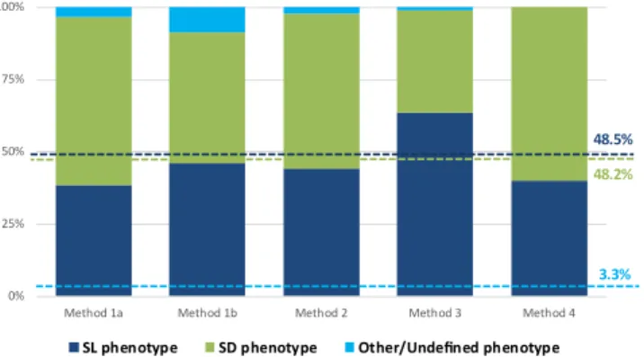
Most of the eligible studies used a single method to identify different sweet taste liker phenotypes; accordingly, a methods-based structure was chosen to organize the eligible papers, versus a purely chron-ological summary. For each method, the relevant studies are discussed and their main characteristics are summarized in a table (Tables 1–5). In cases that used more than one method on the same group of parti-cipants, those studies are included in the relevant tables for each method they used. To assess the impact of these different approaches on phenotype identification, the proportions of the main sweet taste liker phenotypes are graphically presented (Fig. 2). A discussion of the strengths and weaknesses of each classification approach follows, along with recommendations for future research.
2.3. Statistical analysis
Across the studies reviewed, the proportions of individuals within each phenotype varied. These differences could be due to either the sensitivity of the method, or may reflect underlying differences in characteristics of the participant cohort being tested. To assess these hypotheses, two-tailed Z-tests for independent samples (Formula 1) were conducted to determine whether sweet taste liker phenotypes and sex significantly differed across classification methods. The formula used considers the best available estimate for the variance of each pairwise difference under the null hypothesis. Differences in age and BMI between methods were estimated by non-parametric Kruskal Wallis tests (H) for independent samples, followed by Mann Whitney post-hoc tests with adjusted p-values. To account for the different sample sizes, raw age and BMI mean values were transformed into z-scores before these analyses (Formula 2). Effect sizes were calculated for the pairwise comparisons by dividing the Z statistic of the Mann Whitney test with the squared root of the study samples being relevant to each comparison (Field, 2013). Participants’ characteristics are re-ported as percentages in case of categorical variables and as means (M) ± standard deviations (s.d.) for continuous data. All values were
weighted based on the different sample sizes as seen below (Formula 3–5). = + = = + + Z P P P P H P P and P N P N P N N ( ) (1 )
for null hypothesis ( ) : N N 1 2 1 1 0 1 2 1 1 2 2 1 2 1 2
Formula 1.Equation for z-statistic for independent proportions (Z) =
Zscore M M
s d. . pooled
Formula 2.Equation for z-score estimation (Z score)
= + + + + + + P N P N P N P N N N pooled k 1 1 2 2 k k 1 2
Formula 3.Equation for pooled percentage estimation (Ppooled)
= + + + + + + M N M N M N M N N N pooled k 1 1 2 2 k k 1 2
Formula 4.Equation for pooled mean estimation (Mpooled)
= + + + + + + s d N s d N s d N s d N N N k . . ( 1) . . ( 1) . . ( 1) . . ( ) pooled k k k 1 12 2 22 2 1 2
Formula 5. Equation for pooled standard deviation estimation (s.d.pooled)where:
– P1, P2, …, and Pkare the samples’ proportions that have the char-acteristic in question
– N1, N2, …, and Nkare the samples’ size – k is the number of independent samples – M is the mean
– s.d. is the standard deviation
Studies with missing or incomplete data and those using in-compatible measures (e.g. BMI percentiles or categories instead of BMI
Table 6
Z statistics for pairwise comparisons of sex proportions across the different sweet taste liker classifications methods.
% male Method 1a (N= 1290) Method 1b (N= 1335) Method 2 (N= 2591) Method 3 (N= 1990) Method 4 (N= 82)
Z p Z p Z p Z p Z p Method 1a 35.5 0.00 1.000 −3.24 0.001 9.16 < 0.001 −7.89 < 0.001 0.87 0.384 Method 1b 29.6 3.24 0.001 0.00 1.000 12.85 < 0.001 −4.36 < 0.001 2.04 0.041 Method 2 51.1 −9.16 < 0.001 −12.85 < 0.001 0.00 1.000 −19.41 < 0.001 −1.93 0.054 Method 3 22.9 7.89 < 0.001 4.36 < 0.001 19.41 < 0.001 0.00 1.000 3.64 < 0.001 Method 4 40.3 −0.87 0.384 −2.04 0.041 1.93 0.054 −3.64 < 0.001 0.00 1.000 Notes Z, Z-statistic;p,p-value.
Bold text indicates a significant difference with a p-value less than 0.05.
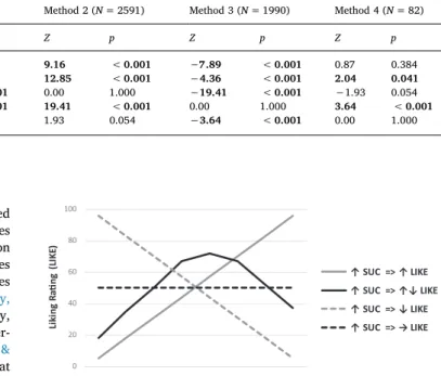
0 20 40 60 80 100 Li ki ng R ati ng ( LIK E)
Sucrose Concentration (SUC)
↑ SUC => ↑ LIKE ↑ SUC => ↑↓ LIKE ↑ SUC => ↓ LIKE ↑ SUC => → LIKE
Fig. 1.Graphical representation of the most commonly reported sweet taste liker phenotypes as they are illustrated by methods interpreting the shape of hedonic response curves.
raw values, median instead of mean values, etc.) were excluded from analysis. To ensure the independence of the various study cohorts, studies with stated or suspected overlap in sampling were excluded. All formula-based calculations were performed in Microsoft Excel 2013 software for Windows. Remaining analyses were carried out using IBM SPSS Statistics version 24.0. An alpha level of .05 was considered for all statistical tests.
3. Results
3.1. Identification of key methodological approaches to classifying sweet taste liker phenotypes
Our literature search identified sixty nine relevant papers describing seventy one studies that met the eligibility criteria including fourteen manually retrieved from the reference lists of the search results; 256 records in Scopus and 192 records in MEDLINE/PubMed were excluded after the screening process was completed. After adjusting for possible overlapping samples, 7543 subjects (37% men; data from 61 studies) who were tested for their hedonic responses to sweet taste and classi-fied to different sweet taste liker phenotypes were included into the final analysis. All but six studies recruited only adults. Average age and BMI for adults were 31.9 years (s.d.= 10.3 years; data from 46 studies) and 26.9 kg/m2(s.d.= 6.6 kg/m2; data from 24 studies), respectively. Research groups from the United States published the most (63%), followed by studies in the UK and elsewhere.
Across the eligible papers four different classification methods were identified: 1a. Visual discrimination of hedonic responses to multiple sucrose concentrations (N= 23 including 2 studies that used two classification methods; Table 1) where individual liking ratings are plotted as a function of concentration, 1b. Statistical discrimination of hedonic responses to multiple sucrose concentrations (N= 5;Table 2) where participants are statistically merged to homogenous groups based on their hedonic responses, 2. The ‘highest preference using ratings’ method (N= 32; Table 4) where the specific sucrose con-centration associated with the highest liking rating was identified, 3. The ‘average liking above mid-point’ or ‘positive/negative liking’ method (N= 10 including 1 study that used two classification methods; Table 4) where liking ratings are compared to a particular cut-off score, and 4. The ‘highest preference via paired comparisons’ method (N= 5 including 1 study that used two classification methods;Table 5) where the sucrose concentration of optimal palatability is identified. These different approaches are described in detail in the subsequent sections. Study populations also vary across methods. One reason for this is that some methodological approaches tend to be used consistently in particular academic fields of study. For example, Method 2 has been widely used in studies relating sweet taste responses to medical con-ditions such as alcoholism, a disorder being more prevalent among males (NSDUH, 2017). In contrast, Methods 1b and 3 are often used by researchers investigating different aspects of sweet-liking such as as-sociations with other sensory characteristics in healthy (i.e. medication free) non-smoking individuals and, correspondingly, young (Kantor, Rehm, Haas, Chan, & Giovannucci, 2015; Moody & Mindell, 2017) women (Jamal et al., 2016; OPN, 2018) of relatively low BMI (Conolly & Saunders, 2017; Fryar, Carroll, & Ogden, 2016) dominate in those cohorts. Accordingly, as can be seen inTable 6, sex distribution differed significantly between methods across all but two pairwise comparisons (Method 4vs. Method 1a:Z= 0.87,p= .384; Method 4vs. Method 2: Z = 1.93, p = .054; p< 0.05 for remaining comparisons). Just over half of those who were assessed via the ‘highest preference’ rating method were men (51.1%), whereas the largest sex disparity was ob-served in studies using the ‘average liking above mid-point’/’positive/ negative liking’ method with barely one out of 4 participants being men (22.9%). Likewise, BMI and age were significantly different across the various classification methods, H(3) = 12.30, p= .006, and H (3) = 9.37, p= .025, respectively. Note that because full data were
only available from a study testing a paediatric population, Method 4 was not included in these comparisons. Follow-up analysis indicated that in studies using Method 2, participants had a considerably greater body size compared to those in Method 1a (p= .001,r= .583), and participants tested were also significantly older than those in Method 1a and 3 (p= .014,r= .299;p= .013,r= .363, respectively). Method 3 tended to test individuals with a lower BMI when contrasted with Method 1b (r= .756, p= .064). Overall, comparisons of age yielded slightly smaller effect sizes relative to the BMI contrasts.
3.2. Classification by interpreting the shape of individual hedonic response curves (Method 1a & Method 1b)
The interpretation of the shape of individual hedonic response curves to different sweet taste stimuli was the first methodology used to identify distinct sweet taste liker phenotypes, following a seminal re-port by Pangborn (1970). In brief, liking ratings (or average liking ratings in case of replicates) across different stimuli are plotted so that the effects of increasing sucrose concentration (x-axis) on the perceived liking at individual level (y-axis) can be visually inspected. A simplified summary of the most commonly reported sweet taste liker phenotypes resulting from visual inspection of the shape of these individual hedonic response curves is shown inFig. 1.
3.2.1. Visual discrimination of hedonic responses to multiple sucrose concentrations (Method 1a)
Simple visual interpretation of response curves to classify partici-pants into different groups presumed to reflect different sweet taste liker phenotypes prevailed for more than four decades (Table 1). In 1970, Pangborn observed three distinct hedonic responses to increasing sucrose concentrations among men: increased liking (‘like’), increased disliking (‘dislike’), and increasing liking ratings followed by a reduc-tion for solureduc-tions with added sucrose above 0.094 M ('like-dislike': Pangborn, 1970). When a range of stronger sucrose solutions was pre-sented to an age diverse population including both men and women, although the intermediate (‘like-dislike’) phenotype was associated with a three times higher breakpoint, an otherwise consistent set of results was revealed (Enns, et al., 1979). Specifically, the ‘liker’ phe-notype was dominant in both experiments (55.0 and 63.3%, respec-tively), while the remaining of the participants were split roughly equally between the two other phenotypes. Age and sex differences aside, participants inPangborn (1970)also tasted nearly twice as many solutions (replicates included) as those inEnns et al. (1979); adaptation (Lawless & Heymann, 2010) and sensory specific satiety (Rolls, Rolls, Rowe, & Sweeney, 1981) could, then, partially explain the qualitative difference observed regarding the intermediate phenotype. A sub-sequent study exclusively in women using a similar range of sucrose concentrations as Enns et al. (1979) but reporting a sucrose con-centration breakpoint closer to that ofPangborn (1970), identified the same three sweet taste liker phenotypes, but failed to confirm these particular proportions (Franko, Wolfe, & Jimerson, 1994). Half of those women had a current diagnosis of bulimia nervosa which is likely to underlie altered or biased sensory evaluations (Drewnowski, 1989).
Those three sweet taste liker phenotypes continue to be reported in more recent studies (Table 1). However, participants who exhibit either an increasing disliking or an inverted U-shaped hedonic pattern are now typically considered as a single group, the SD phenotype. Inter-estingly, although relevant cohorts mainly consisted of young women of normal body weight and the concentration range of sweet taste stimuli tested was relatively similar, the representation of SL-SD phenotypes significantly varied: it ranged between 3:1 inYeomans et al. (2007)to 1:5 inHolt et al. (2000), with almost a 50–50 proportion observed elsewhere (Drewnowski, Henderson, Shore, & Barratt-Fornell, 1997; Oleson & Murphy, 2017). This lack of concordant findings with regard to the number of SLs and SDs identified in studies where this over-simplifying merging occurred, is probably indicative of the implications
of the subjectivity attached to visual inspection-dependent methods. In contrast,Thompson et al. (1976)recognized only two different phenotypes when they visually interpreted the hedonic response curves to sweet taste stimuli; an inverted U-shaped curve characterized by an increased liking up to a sucrose concentration equal to 0.30 M and then a decline (Type I response/phenotype) and an increased liking with concentration (Type II response/phenotype). When they replicated their protocol in another sample of young adults, a similar 70:30 Type I to Type II sweet taste liker phenotypes proportion to that of Group 1 in Thompson et al. (1976) was observed (Thompson, Moskowitz, & Campbell, 1977). In the other studies that used the same classification methodology (Drewnowski & Schwartz, 1990; Grinker & Hirsch, 1972; Johnson, Keane, Bonar, & Downey, 1979; Malcolm, et al., 1980; Thai, et al., 2011; Travers et al., 1993), different proportions of Type I and Type II responders, or sweet dislikers (SDs)-sweet likers (SLs) as they were subsequently renamed byDrewnowski and Schwartz (1990)were reported. It should be noted, though, that except the comparable su-crose concentration breakpoint observed in the Type I responders (0.18–0.32 M), participant characteristics greatly varied across the different studies (Table 1).
A potentially replicable methodology was suggested when the SL-SD classification was attributed to individuals exhibiting a simple mono-tonically ascending and monomono-tonically descending hedonic function to increasing sucrose concentration; SLs were systematically outnumbered by SDs (Drewnowski, Henderson, Shore, & Barratt-Fornell, 1998; Drewnowski, Henderson, & Shore, 1997; Eikemo et al., 2016; Grinker, 1977; Looy, et al., 1992; Looy & Weingarten, 1991, 1992). It is note-worthy that in the studies by Looy and colleagues, although additional sweet taste liker phenotypes were also identified, no further details on those subjects exhibiting either a neutral, an erratic, or an inverted U-shaped response were provided.
3.2.2. Statistical discrimination of hedonic responses to multiple sucrose concentrations (algorithmic classification: Method 1b).
To overcome the possible limitations resulting from the subjective visual discrimination of the different sweet taste liker phenotypes, a statistically-based approach has been suggested recently (Table 2). The hierarchical cluster analysis (HCA) technique produces relatively homogeneous sub-groups (clusters) of cases based on selected char-acteristics either through an agglomerative (successive fusion of in-dividuals into groups) or a divisive (successive separation of inin-dividuals into finer groups) approach (Everitt, Landau, Leese, & Stahl, 2011). Essentially, this method determines how many likely clusters of data are present in the dataset based on the statistical relationship between liking ratings and sucrose concentration for each individual. Wherever the information has been available (Asao, et al., 2015; Garneau, Nuessle, Mendelsberg, Shepard, & Tucker, 2018; Methven, et al., 2016), the agglomerative method was selected, i.e. hierarchical decomposition was formed in a “bottom-up” fashion.
Researchers in Korea were the first to introduce the use of HCA in the relevant literature (Kim, Prescott, & Kim, 2014). In their initial experiment in a sample of young healthy Korean women three clusters were recognized: two clusters where both the hedonic response curves followed the inverted U-shaped pattern but with different breakpoints (0.35 and 0.70 M), and one with increasing liking with increasing su-crose concentration (Kim et al., 2014). It should be noted that in Cluster 2 the gap between the highest and the lowest ratings was only 2 points, similar to the neutral response noted using the visual inspection method discussed earlier. When the protocol was replicated in a comparable study sample (Kim, Prescott, & Kim, 2017), five clusters were reported and interpreted as three distinct sweet taste liker phenotypes evenly distributed across participants. However, unlike their first experiment, only one inverted U-shaped pattern was observed with the maximum liking at 0.35 M. A strong disliking (SDs) and a strong liking (SLs) pattern were also reported each representing approximately one third of the study sample.
Irrespective of the divergent representation of the distinct sweet taste liker phenotypes, the relatively steep increasing slope with in-creasing sucrose concentration (SL phenotype) was also consistent across the rest of the experiments using HCA (Table 2). In a US-based large-scale study of 953 participants from various ethnicities and age groups (Garneau et al., 2018) children’s hedonic responses were clas-sified into two clusters: a SL cluster representing 3 out of 4 children and a second cluster for those with a SD phenotype. HCA for the adults’ sub-group revealed an additional cluster that included both individuals with a relatively neutral liking pattern and those with the inverted U-shaped hedonic response (40.3% and 17.7% of the total adult sample, respec-tively). InMethven et al. (2016)where only two clusters of hedonic responses were identified among UK adults, there were almost half as many SLs as there were SDs. It is worth mentioning that ratings for the two lower sucrose concentrations were only slightly above neutral across those SDs. Another study with a similar small sample size as that inMethven et al. (2016)but which used double the number of sweet taste stimuli, reported an equal number of SLs and SDs in a US cohort (Asao et al., 2015). SD phenotype was, however, expressed by a definite inverted U-shaped hedonic response curve.
3.3. Highest preference using ratings classification method (Method 2) Identifying the sweet taste stimuli associated with the highest pre-ference using ratings from a small set of samples (seeTable 3for the range of stimuli used) and accordingly assigning participants into par-ticular sweet taste liker phenotypes is another commonly used classi-fication method. Following the lead of Kampov-Polevoy and colleagues as originators of this approach (Kampov-Polevoy, Garbutt, Davis, & Janowsky, 1998; Kampov-Polevoy, Garbutt, & Janowsky, 1997), most subsequent studies investigating links between sweet liking and ad-dictive behaviors or mental disorders have used a similar approach. Two distinct sweet taste liker phenotypes were described: a SL pheno-type and a SD phenopheno-type. The SL phenopheno-type was defined as preferring the highest sucrose concentration (or the two higher sucrose con-centrations) typically being at 0.83 or 0.97/0.99 M, whereas subjects rating one of the remaining concentrations (or one of the two lower concentrations) as the most likable were classified as SDs.
A first screening for addiction-related experiments listed inTable 3 revealed that in 6 out of 8 studies under a case-control design that tested participants with a diagnosed alcohol or substance dependence, SLs represented more than 50% of the total study sample ( Bogucka-Bonikowska et al., 2001; Kampov-Polevoy et al., 1997; Krahn et al., 2006; Kranzler, Sandstrom, & Van Kirk, 2001; Tremblay, Bona, & Kranzler, 2009; Wronski et al., 2006). Notably, in half of those studies, the classification criteria that were used for the identification of the distinct sweet taste liker phenotypes may influence the final count in favor of the SL group. For example,Kampov-Polevoy et al. (1997) and Kranzler et al. (2001)attributed the SL phenotype to subjects expres-sing preference for either the first or the second highest sucrose con-centration, whileTremblay et al. (2009)used a much stricter definition for the SDs (maximum liking rating for the lowest sucrose concentra-tion). The two remaining addiction-related studies are split between those where the two discrete sweet taste liker phenotypes were evenly distributed across participants (Bogucka-Bonikowska et al., 2002), and those where SLs were less than one third of the total study sample (Kampov-Polevoy et al., 1998).
Regarding studies testing psychiatric patients and their matched healthy controls, regardless of the heterogeneity in age and underlying disorders, less variability among the proportions of the distinct sweet taste liker phenotypes was reported. In these studies, SLs were either more than (Sienkiewicz-Jarosz et al., 2013; Swiecicki et al., 2015; Swiecicki et al., 2009) or as many as (Damiano et al., 2014) the SDs in all but one (Dichter, Smoski, Kampov-Polevoy, Gallop, & Garbutt, 2010) study. Unlike with the addiction-related trials, women overall outnumbered men, while inSienkiewicz-Jarosz et al. (2013), Swiecicki