Subsymbolic methods for data mining in
hydraulic engineering
Anthony W. Minns
Anthony W. Minns
International Institute for Infrastructural, Hydraulic and Environmental Engineering (IHE), P.O. Box 3015,
2601 DA Delft, The Netherlands E-mail:[email protected] ABSTRACT
This paper describes the results of experiments with artificial neural networks (ANNs) and genetic programming (GP) applied to some problems of data mining. It is shown how these subsymbolic methods can discover usable relations in measured and experimental data with little or noa priori knowledge of the governing physical process characteristics. On the one hand, the ANN does not explicitly identify a form of model but this form is implicit in the ANN, being encoded within the distribution of weights. However, in cases where the exact form of the empirical relation is not considered as important as the ability of the formula to map the experimental data accurately, the ANN provides a very efficient approach. Furthermore, it is demonstrated how numerical schemes, and thus partial differential equations, may be derived directly from data by interpreting the weight distribution within a trained ANN. On the other hand, GP evolutionary force is directed towards the creation of models that take a symbolic form. The resulting symbolic expressions are generally less accurate than the ANN in mapping the experimental data, however, these expressions may sometimes be more easily examined to provide insight into the processes that created the data. An example is used to demonstrate how GP can generate a wide variety of formulae, of which some may provide genuine insight while others may be quite useless.
Key words| artificial neural networks, data mining, genetic programming, subsymbolic methods
INTRODUCTION
Data mining constitutes one part of the multi-step knowledge-discovery process for extracting useful pat-terns and models from raw data stores. Fayyadet al.(1996,
p. 44) describe a variety of data mining procedures that include:
•
classification:in which a function is learned that maps (classifies) a data item into one of several predefined classes;•
regression:in which a function is learned that maps a data item to a real-valued prediction variable;•
clustering:in which one seeks to identify a finite set of categories or clusters to describe the data;•
summarisation:in which a compact description isfound for a subset of the data;
•
dependency modelling:in which a model is found that describes significant dependencies between variables;•
change and deviation detection:which focuses on discovering the most significant changes in the data from previously measured or normative values. The other steps in the knowledge discovery process are those of data preparation, data selection, data cleaning, the incorporation of appropriate prior knowledge and the proper interpretation of the discovered results. Knowledge is only useful if it is in a form that can be accessed and used reliably by different people. The raw data involved here are usually so numerous that the more traditional, manual methods of data mining must now make way for computer-based methods, which are much better suited tounearthing meaningful patterns and structures from vast databases rapidly and reliably.
The goal of the knowledge discovery steps may be simply to condense the data into a short, printed report, or it may be to find a model of the process that generated the data and which may be used to estimate values in future cases. The fitted models play the role of inferred knowl-edge. This is similar to the problem of systems investi-gation, or systems identification, defined as the field of study which is concerned with the direct solution of technological problems subject only to the constraints imposed by the available data and so not subject to ‘physi-cal’ considerations (Amorocho & Hart1964).
Following Iba et al. (1993), we may define systems
identification in the following way. Imagine that a system produces an output value,y, and that thisyis dependent onminput values, thus:
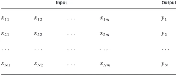
y=f(x1,x2,x3, . . . ,xm). (1) Given a set ofNobservations of input–output tuples, as shown in Table 1, the system identification task is to approximate the true function f with an approximating functionf.
Once this approximate functionfhas been estimated, a predicted outputycan be found for any input vector (x1,
x2. . .xm) from:
y=f(x1,x2,x3, . . . ,xm). (2) The f is called the complete form of f. As pointed out by Minns (1998a), artificial neural networks (ANN)
constitute one class of sub-symbolic paradigms that lends itself very easily to the problem of searching for and storing the complete form off.
An ANN is an electronic knowledge encapsulator that encapsulates its knowledge at the level of thetaxonomia by establishing some useful relation between a collection of signs on the input side and a collection of signs on the output side. The actual relation is stored electronically at the subsymbolic level as a series of weights and connec-tions between nodes. It is usually not possible to extract and interpret an exact, symbolic, mathematical formu-lation of this reformu-lation. At the level of the mathesis, this relation becomes extremely complex owing to the non-linear nature of the transformations that take place upon the weighted sums of the signals through the application of sigmoid threshold functions.
Artificial neural networks provide an extremely powerful paradigm for only some of the data mining procedures mentioned above (e.g. classification and regression). In some other procedures, the use of the existing types of ANNs may be entirely inappropriate. This paper describes the performance of ANNs when applied to various problems of data mining and system identifi-cation. Some of the results are compared to the results obtained from more traditional manual methods, as well as some other computer-based methods. In particular, a comparison is made with results obtained from another subsymbolic approach called genetic programming (GP).
GP is one of the evolutionary algorithms that can actually generate models in a symbolic form (Koza1992).
Whereas traditional genetic algorithms typically operate by combining binary strings which encode real-valued independent variables (see, for example, Babovic1993), in
the case of GP, the symbolic expressions themselves are subject to the genetic operators of recombination and mutation (Babovic & Abbott1997). In this way GP may, at
first, appear to be entirely symbolic in nature. This is, however, not at all true. As explained by Babovic (1996,
p. 248), both ANNs and GP are subsymbolic in the sense that a manipulation of data occurs at a level which is below that of the symbol. The tokens that are manipulated are, at best,indicative signs, but do not have any expres-sivecapability in and by themselves. GP manipulates tree
Table 1| An input–output example set.
Input Output
x11 x12 . . . x1m y1
x21 x22 . . . x2m y2
. . . .
structures that only acquire any meaning, or semantic content, once the tree has been interpreted as an algebraic expression in Reverse Polish Notation, or prefix notation, of standard computer science (Babovic & Abbott 1997,
p. 402).
GENERATION OF EQUATIONS FROM DATA
Minns (1998a,b) showed that, in the simplest case of pure
advection with a constant velocity, a linear ANN (i.e. a multi-layer perceptron with linear threshold functions) is capable of learning the exact solution, which is also exactly equivalent to the partial differential equation description, from only discrete measured data points. The ANN in fact functions as a numerical operator that con-tains the same knowledge, or has the same semantic content, as the governing partial differential equations. It was shown that the governing continuum equations could actually be restored by analysing the weights of the ANNs that are trained with the measured data. This procedure was extended by Dibike et al. (1999) to the problem of
simple, short-period wave equations. The usual pro-cedures of numerical modelling were adapted in these studies to become a knowledge discovery procedure as schematised in Figure 1.
This procedure can be applied to the problem of modelling the advection and dispersion of a conservative pollutant along a channel. The basic continuum equation for the advection-dispersion process in one dimension is:
wherec is the concentration of pollutant (mg/l),u is the velocity (m/s) andDis the dispersion coefficient (m2/s).
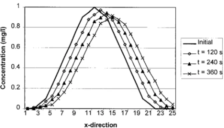
In order to demonstrate the validity of the above knowledge discovery procedure, a set of data describing the advection and dispersion of a cloud of pollutant along a channel had to be collected. For this experiment, these data were generated using the MIKE11 modelling system of the Danish Hydraulic Institute, which uses equation (3) for modelling advection–dispersion (AD) processes. The data could be therefore generated for ‘known’ pre-determined values ofuandD.The objective of the exper-iment is then to regenerate equation (3), together with the correct values ofuandD, from the ‘raw’ data alone.
The concentration profile generated using MIKE11 is shown in Figure 2 for three consecutive timesteps. These results were obtained using a velocity of 0.833 m/s, a dispersion coefficient of 50 m2/s, a grid size of∆x= 100 m and a timestep of∆t= 120 s. The velocity, grid size and timestep were chosen carefully so that the Courant number, defined as Cr=u ∆t/∆x, was equal to 1.0. The numerical results were therefore free from the effects of numerical diffusion or dispersion.
Figure 1|Schematisation of (a) the usual procedures of numerical modelling and (b) the
knowledge discovery procedure (adapted from Dibikeet al.1999, p. 82).
(a) (b) NUMERICAL MODELLING PROCEDURE KNOWLEDGE DISCOVERY PROCEDURE Partial differential equation Data=
{set of numbers in space and time}
↓ ↓
Taylor series ANN weights
↓ ↓
Finite difference scheme Finite difference scheme
↓ ↓
Solution algorithm Taylor series
↓ ↓
Solution= {set of numbers in
space and time}
Partial differential
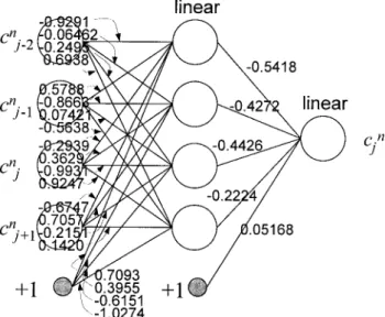
The value of the concentration at any general gridpointjat any time levelnmay be denoted ascn
j. The values in the gridpoints immediately adjacent to this point on the left and right are then denoted as cn
j− 1 andcnj+ 1 respectively. The value of the concentration at the grid-pointjat the following time step is denotedcn+ 1
j . A set of input-output tuples, as described in Table 1, was then created from these data with cn
j− 2, cnj− 1, cnj and cnj+ 1 as inputs andcn+ 1
j as the single output. A tuple was created for each gridpoint for three consecutive timesteps. This gave a total of 85 tuples.
A linear ANN was then trained on this data using the standard methods of error-backpropagation (Rumelhart et al. 1986). This network rapidly converged to a small
residual error and the final distribution of weights that were obtained after training is shown in Figure 3.
The configuration of the ANN in Figure 3 can be expressed mathematically as:
cn+ 1 j = − 0.5418[ − 0.9291cnj− 2+ 0.5788cnj− 1 − 0.2939cn j − 0.6747cnj+ 1+ 0.7093] − 0.4272[ − 0.06462cn j− 2− 0.8663cnj− 1 + 0.3629cn j + 0.7057cnj+ 1+ 0.3955] − 0.4426[ − 0.2495cn j− 2+ 0.07421cnj− 1 − 0.9931cn j − 0.2151cnj+ 1− 0.6151] − 0.2224[0.6938cn j− 2− 0.5638cnj− 1 + 0.9247cn j + 0.1420cnj+ 1− 1.0274] + 0.05168
that reduces to: cn+ 1
j = 0.4871cnj− 2+ 0.1490cnj− 1+ 0.2381cnj + 0.1278cn
j+ 1− 0.0008. (4)
It is apparent in equation (4) that the value of the constant term is almost zero and can therefore be neglected. Taylor series expansions of the terms in equation (4), about the centre point of the scheme at (j∆x, n∆t), provide the following expansions:
where ‘hot’ stands for higher-order terms in the Taylor series expansion. The terms in equation (5) can be substituted into equation (4) to obtain:
Rearranging the terms in equation (6) and dividing by∆t then leads to:
We see that the coefficient in front of the last term in equation (7) is extremely small so that thecn
j term can be neglected.
Now if we differentiate equation (3) once with respect to x and once with respect to t, and then subtract the two resulting expressions in order to cancel the cross derivative terms, and then neglect the terms that are of third-order and above, we get the following order relation:
Substituting equation (8) into equation (7) then provides the expression:
which is obviously an advection–dispersion equation of the same form as equation (3) and with an expression for the velocityu =0.9955∆x/∆t. Substituting this expression for the velocity into the dispersion coefficient on the right-hand side of equation (9) results in an advection– dispersion equation of the form:
where
u= 0.9955∆x/∆t (11)
and
D= 0.6172∆x2/∆t. (12)
Substituting our values of∆x= 100 m and∆t= 120 s into equations (11) and (12) we obtain values for the velocity and dispersion coefficient of u= 0.830 m/s and D= 51.4 m2/s respectively. These values compare very closely with the actual values ofu= 0.833 m/s and D= 50 m2/s that were originally used to generate the data.
These results confirm that it is possible to derive numerical schemes and thus partial differential equations
directly from raw data using ANNs as data mining tools. Dibike et al. (1999) further argue that if numerical
sol-utions of partial differential equations are used to provide the data sets that are used to train the ANNs, and the resulting weights of the ANNs are able to reinstate the original differential equations, then data taken from nature should just as well provide ANNs that can in turn produce partial differential equation descriptions of the natural processes. The results of this analysis then go some way toward refuting the scepticism of the ‘traditional’ engineering and science community about the ability of artificial neural networks to encapsulate knowledge that has been ‘traditionally’ encapsulated in the form of con-tinuum equations. They also serve to induce a greater confidence in the predictive abilities of ANNs.
RAINFALL-RUNOFF MODELLING
Perhaps one of the fastest growing applications of neural networks to geophysical sciences is in the area of rainfall-runoff modelling. At the time of writing, the author is aware of at least two new books currently in preparation that will be entirely devoted to hydrological applications of ANNs. The general approach to rainfall-runoff model-ling using ANNs has been described extensively by Hall & Minns (1993), Minns (1996, 1998a) and Minns & Hall
(1996,1997).
In particular, Minns & Hall (1996) describe
exper-iments using flow data generated from synthetic storm sequences routed through a conceptual hydrological model. It was shown that the best results were obtained for an ANN with an input array consisting of the concurrent and fourteen antecedent rainfall depths and three ante-cedent flow ordinates. The output consisted of the concur-rent flow ordinate only. The time interval of the input rainfall data broadly encompassed the range of centroid-to-centroid lag times of the catchment. Although the results of these experiments show that an ANN is capable of learning an extremely accurate relation between the runoff ordinates and the antecedent rainfall depths, it is not possible to identify theformof the modelling relation thus obtained. As shown in the previous section, the form
of the model is implicit in the ANN within the distribution of weights and this distribution is obtained automatically with no user intervention. Minns & Hall (1996) refer to the
ANN as theultimate black box.
In an attempt to extract more information about the form of the relation that exists between the input data and the outputs, Babovic (1996, but see also Babovic & Abbott, 1997) performed data mining experiments using genetic
programming on the same rainfall-runoff data created for the Minns & Hall (1996) experiments. Based upon the
results of Minns & Hall (1996), the training data for the GP
were chosen as the concurrent and fourteen antecedent rainfall depths (i.e. [rt, rt− 1,rt− 2, . . . , rt− 14]), as well as two antecedent flow values (i.e. [qt− 1, qt− 2]).The output data consisted only of the concurrent flow valueqt.
After a sufficient number of generations of the GP, two expressions were generated that fitted the training data with fairly similar accuracy. Babovic (1996) gives the
simplified form of these two expressions as: qt= 1.1052qt− 1− 0.1367rt− 12− 0.6636rt− 11
+ 0.0003 (13)
and
qt= 1.1000qt− 1− 0.7214rt− 11− 0.0201rt− 10
− 0.0035. (14)
That is, the GP has found that the entire rainfall-runoff process can be described by a superposition of pure advec-tion processes. (For a more detailed discussion of this interpretation see Babovic & Abbott1997, p. 416.) Purely
from the viewpoint of data mining, the GP has found that only three input variables are necessary to describe the rainfall-runoff modelling process in each case. Regardless of whether one accepts expressions (13) and (14) as being ‘physically realistic’ or not, the GP has achieved one of the primary goals of data mining—that of finding a compact description of the data set. It is now interesting to compare the performance of expressions (13) and (14) with the solution obtained by the three-layer ANN that was trained on the same data by Minns & Hall (1996). The coefficients
of efficiency for the training data sequence and for the verification data sequence are given in Table 2 for the ANN model and for both of the GP expressions.
Table 2 indicates that efficiencies of more than 99% have been achieved for both methods in fitting a function to the given data. The ANN model performs slightly better than the GP expressions on both training and verification data; however, the ANN model requires eighteen input variables, whereas the GP expressions require only three input variables each. As mentioned above, the total time interval of the window of input rainfall data should encompass the centroid to centroid lag times of the catch-ment runoff data. The GP expressions then confirm this conclusion by selecting only the rainfall ordinates with these lag times. All other rainfall ordinates have been neglected by the GP.
It is not possible here, nor even very prudent, to draw conclusions about the superiority of the one method over the other. For example, the advantage of the extra accuracy of the ANN approach in one application may be counteracted by the advantage of the extreme compact-ness of the GP expressions in another. In fact, a truly superior method is most likely to be obtained when the two techniques are combined in a so-called ‘hybrid’ approach. This approach can be demonstrated by con-sidering in more detail how the strengths of each separate technique can be used to enhance the performance of the other.
In the above example, the use of 15 rainfall ordinates in the input data set to the GP was decided upon after several ANN models with different configurations had been tested to discover the optimal length of the input window. This initial testing of a number of variations can be done much more rapidly with an ANN than with GP,
Table 2 |Performance overview in terms of coefficients of efficiency for an ANN model
and for two GP expressions on training and verification data from a synthetic catchment.
Model
Coefficients of efficiency
Training data Verification data
Three-layer ANN 0.9987 0.9941
GP expression(13) 0.9903 0.9926
due to the extreme simulation time required for every application of the GP algorithm as compared to the train-ing time of an ANN. Havtrain-ing established this optimum window length, the input data to the GP were then selected and the resulting expressions (13) and (14) resulted from the evolution process.
Subsequently, expressions (13) and (14) can be used to further enhance the performance of the ANN. For example, expression (13) indicates that a very accurate solution can be found with only the three input variables: rt− 11, rt− 12, and qt− 1. This information was therefore used to configure a new ANN model using only these three input variables. The results of using an ANN model with five hidden nodes, and using sigmoid threshold functions throughout, produced coefficients of efficiency of 0.9915 for the training data and 0.9933 for the validation data. Comparing these results with the coefficients of efficiency given in Table 2, it is seen that these new results are only slightly less accurate than the original ANN model. How-ever, they are still more accurate than the GP expressions, but now utilising the same amount of input data as the GP model. The new ANN model is of course much more compact than the original model and is subsequently much easier and faster to train.
Lastly, it is also possible to use the power of the ANN learning algorithm to improve directly upon the given GP expressions. The linear nature of the GP expressions means that these expressions can be exactly represented by a simple two-layer ANN that uses linear threshold functions. Two linear ANNs were therefore configured and trained using [rt− 11,rt− 12,qt− 1] as input data in the first case, and [rt− 10, rt− 11, qt− 1] as input data in the second case. These small, linear ANNs converged very rapidly using the back-propagation learning algorithm to provide the solutions:
qt= 1.0962qt− 1− 0.5238rt− 12− 0.1812rt− 11
− 0.0845 (15)
in the first case, and:
qt= 1.0970qt− 1− 0.6478rt− 11− 0.0320rt− 10
− 0.1090 (16)
in the second case.
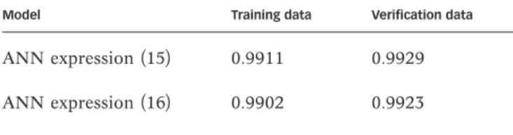
The coefficients of efficiency for expressions (15) and (16) are summarised in Table 3, which can be compared to the results in Table 2 for GP expressions (13) and (14).
The most significant result of this experiment is the extreme similarity that exists between the GP expression (14) and the ANN-induced expression (16). The coef-ficients of efficiency for these expressions differ only very slightly and thus indicate that both the GP and ANN have found the near-optimum values of the coefficients in the linear expression that relates these three input variables. The more significant differences between the GP expres-sion (13) and the ANN-induced expresexpres-sion (15) indicate that the GP had probably not yet arrived at the optimum values for the coefficients in this case. This is not neces-sarily due to an error in the GP algorithm, but rather indicates that the evolutionary process for this particular expression was halted prematurely.
SEDIMENT TRANSPORTATION
Another comparison between the performance of ANNs and GPs in data mining can be made using the results of experiments performed by Minns (1995) and Babovic &
Abbott (1997). The data sets used in this study were taken
from the work of Zyserman & Fredsøe (1994), which were
in turn derived from Guyet al. (1966). This work involved
the determination of the bed concentration of suspended sediment cb from flume experiments. The experimental data provided the total, steady-state sediment load for a range of hydraulic conditions including varying discharge, bed-slope and water depths. Zyserman & Fredsøe (1994)
Table 3 | Coefficients of efficiency for linear ANN models on training and verification data
from a regular catchment.
Model
Coefficients of efficiency
Training data Verification data
ANN expression(15) 0.9911 0.9929
derived the bed concentration of sediment cb for each experiment from the total measured load. The physical set-up and hydraulic conditions of each experiment were described by a set of six parameters incorporating all of the measured data. These parameters wereO,O′,uf,u′f,d
50, and
ws, whereOandO′ are the Shield’s parameters related to the average shear velocityuf and the skin friction shear velocityu′
frespectively, d50is the median grain diameter andwsis the settling velocity of suspended sediment.
In order to derive an expression relating the extremely difficult-to-measure bed concentration,cb, to other, easy-to-measure, hydraulic parameters, Zyserman & Fredsøe applied dimensional analysis techniques to all of the avail-able measured data described above. The resulting rela-tion arrived at by Zyserman & Fredsøe (1994) was given
as:
Expression (17) implies that theonlysignificant parameter for determining the bed concentration is the skin friction Shield’s parameter O′. The discussion of expression (17) given by Zyserman & Fredsøe indicates that this expres-sion gives comparable, if not better, accuracy than several other, more complex, empirical formulations. The ques-tion remains, however, whether this result could be improved by includingallof the measured data instead of only one parameter. Artificial neural networks can be used very easily to assess this hypothesis.
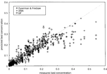
An ANN was subsequently set up with six nodes in the input layer, one node for each of the parameters given above, four nodes in the hidden layer and a single node in the output layer consisting of the bed concentration,cb. The ANN was trained using all of the data that was available to Zyserman & Fredsøe. The results of the train-ing are depicted in Figure 4, which is a scatter plot of the measured bed concentrations compared to the bed con-centrations as calculated by the trained ANN and by the Zyserman & Fredsøe equation (17).
It can be seen from Figure 4 that the ANN has a smaller scatter from the diagonal compared to the results from equation (17), especially for the higher values of bed concentration. To compare the accuracy of the ANN to that of equation (17), the coefficient of efficiency was
calculated for each method. The coefficient of efficiency for the ANN results was 0.905 compared to 0.802 for expression (17). This indicates a significant improvement in the predictive capability on the part of the ANN, as compared to the more traditional approach. Furthermore, the ANN makes use of all of the available data and hence provides a solution that will be sensitive to variations in any of the hydraulic parameters and not justO′ as is the case with equation (17).
An ANN has therefore demonstrated the capacity to discover and learn a relation between easy-to-measure hydraulic flow parameters and the bed concentration of suspended sediment with significantly more accuracy than that achieved by more traditional regression analysis and dimensional analysis techniques. Furthermore, whereas dimensional analysis may reject some hydraulic parameters in order to simplify the resulting expressions, the ANN makes use of all of the available measured data, thus improving the accuracy and sensitivity of the result-ing relation without the need for any preliminary analysis to select the most significant parameters, or to disregard less significant parameters.
A GP analysis of this same data is described in detail by Babovic & Abbott (1997). In this case, the GP performs
slightly better than the dimensional analysis approach, but produces algebraic expressions of remarkably similar form
Figure 4|Scatter plot of bed concentrations calculated by an ANN with six input
parameters compared to results from the Zyserman & Fredsøe equation (17) and the genetic programming derived equation (19).
to expression (17) that again utilise only some of the six parameters that encapsulate all of the measured data. The best performing GP expression was given in algebraic form as:
Further experiments on this same data using the genetic programming tool described by Keijzer & Babovic (1999)
produced many other equations of various forms that significantly outperformed equations (17) and (18). How-ever, very little insight into the processes of sediment transportation could be gained by examining any of these formulae. One of the best performing equations can be written as:
cb= 4u′f− 2ws−u′f((d50+ws)2−O′) −uf. (19) Equation (19) has a coefficient of efficiency of 0.825, which is an improvement over the original Zyserman & Fredsøe expression but still does not approach the accuracy of the ANN. Moreover, the GP has found the simplest expression that contains only the ‘most signifi-cant’ parameters in the relation. The GP has found an expression with correct syntax but with little or no semantic content. The results of Equation (19) are also plotted in Figure 4 for comparison.
Subsequently, Babovic & Keijzer (1999) have
extended GP to produce dimensionally correct formulae during the evolutionary process. This ‘dimensionally aware’ GP produced an expression of the form:
Equation (20) is dimensionally correct and appears to use the most relevant physical properties in the relevant con-text. For example, the dimensionless term u′
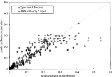
fws/gd50 is effectively a ratio of shear and gravitational forces. This is indeed an improvement over the original formulation of Zyserman & Fredsøe that only involved a relation usingO′. Interestingly enough, if the ANN used above is simpli-fied and trained to calculate cb from only one input parameter, namelyO′, then results are obtained that are of
very similar accuracy to Equation (17). For the sake of comparison, an ANN was trained with only this one input parameter. The scatter plot of the results is illustrated in Figure 5. In this experiment, the ANN results have a coefficient of efficiency of 0.815 and the scatter of points about the diagonal line in Figure 5 is remarkably similar to the results from equation (17).
Now, if equations (17), (18) and (19) are accepted as having no deeper physical meaning (i.e. they have no semantic content), so that they are only computational tools to calculate cb, then the only major difference between these computational tools and the ANN is that equations (17), (18) and (19) can be written down exactly on paper while the ANN is stored, usually electronically, as a series of weights and connections between nodes. The evaluation of equations (17), (18) and (19), however, also requires the use of some sort of modern computational device and so the restriction of ANNs to be used only on computers is not considered as an extraordinarily limiting factor here.
If we compare the accuracy of the ANN model to the accuracies of equations (17), (18) and (19), it becomes clear that the exclusion of even only some of the ‘less significant’ parameters can still affect the overall accuracy of the final solution quite significantly when dealing with the more complex physical relations typical of those that exist in sediment transportation problems. In effect, the
Figure 5|Scatter plot of bed concentrations calculated by an ANN with only one input
GP approach can become subjected to the same limi-tations of a restricted symbol system as does any algebraic system, whereas the ANN, being much more ‘sub-symbolic’, largely escapes from this restriction. For a more complete discussion of the problems of reading a physical ‘meaning’ into equation (17) (18) or (19), refer-ence is made to the paper of Babovic & Abbott (1997,
pp. 416–420).
CONCLUSIONS
It has been shown that subsymbolic methods like artificial neural networks (ANNs) and genetic programming (GP) may be used as data-mining techniques to discover usable relations in measured or experimental data. Experiments have demonstrated the possibility of deriving numerical schemes and thus partial differential equations directly from data by interpreting the weight distribution within a trained ANN. This finding may serve to induce some confidence in the predictive ability of ANNs. GP will generate symbolic-algebraic expressions that also fit the data quite well, however these expressions are not guaranteed to necessarily provide a deeper insight into the underlying physical processes.
A common, more traditional, approach to the analysis of measured and experimental data is through dimen-sional analysis and statistical curve fitting. Generally, the objective of such an analysis is simply to relate quantities that are very difficult to measure outside a specialised laboratory to parameters that can be easily measured in the field. Although the empirical formulae thus derived often fit the experimental data to a high degree of accu-racy, these formulae often present the aspect of extremely complex, nonlinear combinations of parameters and con-stants that do not really give much insight into the physi-cal system being described. In addition, the form and accuracy of the formulae are often very sensitive to the choice of parameters, dimensionless or otherwise. In many cases, for the sake of simplicity, several parameters, and hence measured data, may be disregarded entirely, at the cost of some accuracy in the final formulation of the relation. The fact that the exact form of the empirical
relation is thus not as important as the ability of the formula to map the experimental data accurately indicates that this kind of analysis may be very efficiently carried out using ANNs. Dimensionally-aware GP may provide a better approach to generating more ‘meaningful’ relations. The true strength of the subsymbolic paradigms lies in their ability to identify relations between measured data without requiring a detailed knowledge of physical pro-cess characteristics a priori. The ANN is indeed a ‘very black’ box, where the user of the model has very little (if any) influence upon the form of model to be fitted to the measured data. The ANN does not explicitly identify a form of model but this form is implicit in the ANN, being encoded within the distribution of weights. With tra-ditional conceptual modelling techniques the modeller applies his or her measured data together with some physical insight in order to adjust modelling parameters and equations manually and so eventually to calibrate the model. In ANN modelling, one could almost speak of an automatic calibrationprocedure.
This superior performance characteristic of the ANN paradigm over the more traditional, manual methods of data mining and analysis can also be claimed by genetic programming (GP). Although essentially subsymbolic at its most basic level, GP will supply a symbolic-algebraic relation between the measured data through a process of evolution and competition between all possible solution expressions. An ANN, on the other hand, will usually find a relation between the input and output data that has a much higher accuracy, but then the resulting relations can only be represented subsymbolically and are therefore essentially ‘hidden’ from the user of the model. In certain cases, it has been shown that a ‘hybrid’ approach, which uses the ‘best’ characteristics of both GP and ANNs, can provide even more accurate solutions than just one approach on its own.
ACKNOWLEDGEMENTS
The tool used to produce the genetic programming results in this study was developed under the Talent Project No. 9800463 entitled ‘Data to Knowledge–D2K’ funded
by the Danish Technical Research Council. More informa-tion on the D2K project can be obtained throughhttp:// projects.dhi.dk/d2k.
REFERENCES
Amorocho, J. & Hart, W. E.1964A critique of current methods in
hydrologic systems investigation.Trans. Am. geophys. Un.45,
307–321.
Babovic, V.1993Evolutionary algorithms as a theme in water
resources. InScientific Presentations of AIO Meeting ‘93: AIO
Network Hydrology(ed. R. H. Boekelman), pp. 21–36. Delft
University of Technology, The Netherlands.
Babovic, V.1996Emergence, Evolution, Intelligence;
Hydroinformatics.Balkema, Rotterdam.
Babovic, V. & Abbott, M. B.1997The evolution of equations from
hydraulic data, Parts I & II.J. Hydraulic Res.35(3), 397–430.
Babovic, V. & Keijzer, M.1999Data to knowledge—the new
scientific paradigm. InProceedings of Computing and Control
for the Water Industry, Exeter, U.K.
Dibike, Y., Minns, A. W. & Abbott, M. B.1999Applications of
artificial neural networks to the generation of wave equations
from hydraulic data.J. Hydraulic Res.37(1), 81–97.
Fayyad, U., Piatetsky-Shapiro, G. & Smyth P.1996From data
mining to knowledge discovery in databases.AI Magazine
(American Association for Artificial Intelligence)17(3), 37–54.
Guy, H. P., Simons, D. B. & Richardson, E. V.1966Summary of
alluvial channel data from flume experiments:1956–61.
Professional Paper 462-I, U.S. Geological Survey, Washington, D.C.
Hall, M. J. & Minns, A. W.1993Rainfall-runoff modelling as a
problem in artificial intelligence:experience with a neural
network. InProceedings of the 4th National Hydrology
Symposium, Cardiff, pp. 5.51–5.57. British Hydrological
Society, London.
Iba, H., de Garis, H. & Sato, T.1993Solving Identification Problems
by Structured Genetic Algorithms. ETL-TR-93–17.
Keijzer, M. & Babovic, V.1999Dimensionally aware genetic
programming. InProceedings of the Genetic and Evolutionary
Computation Conference, GECCO ‘99, Orlando, Florida.
Koza, J.1992Genetic Programming: On the Programming of
Computers by Means of Natural Selection.MIT Press,
Cambridge, MA.
Minns, A. W.1995Analysis of experimental data using artificial
neural networks.HYDRA 2000, Proc. XXVI Congress IAHR,
London, Vol. 1, Thomas Telford, London, pp. 218–223.
Minns, A. W.1996Extended rainfall-runoff modelling using artificial
neural networks.Hydroinformatics ‘96, Proc. 2nd International
Conference on Hydroinformatics, ETH-Zu¨rich, pp. 207–213.
Balkema, Rotterdam.
Minns, A. W.1998a Artificial Neural Networks as Sub-symbolic
Process Descriptors. Balkema, Rotterdam.
Minns, A. W.1998bModelling of 1-D pure advection processes
using artificial neural networks. InHydroinformatics ‘98, Proc.
3rd International Conf. on Hydroinformatics,Copenhagen(ed.
V. Babovic & L. C. Larsen), vol. 2, pp. 805–812. Balkema, Rotterdam.
Minns, A. W. & Hall, M. J.1996Artificial neural networks as
rainfall-runoff models.J. hydrolog. Sci.41(3), 399–417.
Minns, A. W. & Hall, M. J.1997Living with the ultimate black box:
more on artificial neural networks. InProceedings of the 6th
National Hydrology Symposium, Salford, pp. 9.45–9.49. British
Hydrological Society, London.
Rumelhart, D. E., McClelland, J. L. & PDP Research Group1986
Parallel Distributed Processing–Explorations in the
Microstructure of Cognition.Two volumes. MIT Press,
Cambridge, MA.
Zyserman, J. A. & Fredsøe, J.1994Data analysis of bed
concentration of suspended sediment.J. hydraul. Engng120(9),