NBER WORKING PAPER SERIES
DO TRUST AND TRUSTWORTHINESS PAY OFF?
Joel Slemrod Peter Katuscak
Working Paper 9200
http://www.nber.org/papers/w9200
NATIONAL BUREAU OF ECONOMIC RESEARCH 1050 Massachusetts Avenue
Cambridge, MA 02138 September 2002
We would like to thank members of the University of Michigan Public Finance workshop, and particularly John Bound and Matthew Shapiro, for helpful comments on an earlier version of this paper. The views expressed herein are those of the authors and not necessarily those of the National Bureau of Economic Research.
© 2002 by Joel Slemrod and Peter Katuscak. All rights reserved. Short sections of text, not to exceed two paragraphs, may be quoted without explicit permission provided that full credit, including © notice, is given to the source.
Do Trust and Trustworthiness Pay Off? Joel Slemrod and Peter Katuscak NBER Working Paper No. 9200 September 2002
JEL No. J30, H40
ABSTRACT
Are individuals who trust others better off than those who do not? Do trustworthy people prosper more than untrustworthy ones? We first pose these questions in a search model where individuals face repeated choices between trusting (initiating an investment transaction) and not trusting, and between being trustworthy (not stealing the investment) and cheating. We then derive predictions for the relationship between observed individual behavior, aggregate attitudes, and individual prosperity. Finally, we evaluate these predictions empirically using household-level data for eighteen (mostly developed) countries from the World Values Survey. We find that, on average, a trusting attitude has a positive impact on income, while trustworthiness has a negative impact on income. In addition, we find evidence of complementarity between these two attitudes and the aggregate levels of the complementary attitudes. Most strikingly, the payoff to being trustworthy depends positively on the aggregate amount of trust in a given country.
Joel Slemrod Department of Economics University of Michigan and NBER E-mail: [email protected] Peter Katuscak Department of Economics University of Michigan E-mail: [email protected]
1
Introduction
The notions of trust and trustworthiness have received much recent attention in social science, stimulated in part by the work of Putnam (1993) and Fukuyama (1995), but with antecedents in, for example, Coleman (1990). Economists have for a long time recognized the critical role played by trust in economic performance. Arrow (1972), for example, remarks: “Virtually every commercial transaction has within itself an element of trust, certainly any transaction conducted over a period of time. It can plausibly be argued that much of the economic backwardness in the world can be explained by the lack of mutual confidence.” In high-trust societies, individuals need to spend less resources to protect themselves from being exploited in economic transactions. Knack and Keefer (1997) argue that trusting societies tend to have stronger incentives to innovate and to accumulate both physical and human capital and, as a result, grow faster. Zak and Knack (2000) corroborate the positive effect of aggregate trust on growth. Alesina and La Ferrara (2000) investigate the individual-level determinants of trust within the United States and find that income and education are strongly positively correlated with trust.
The flip side of trust is trustworthiness. Glaeser et al (2000) distinguish between trusting behavior, which they define as “the commitment of resources to an activity where the outcome depends upon the cooperative behavior of others,” and trustwor-thy behavior, which “increases the returns to people who trust you.” The idea of reputation–the level of trust one is perceived to merit–has also been examined. As Axelrod (1986) puts it, an individual’s reputation derives from adherence to or
vio-lation of a norm that others view as a signal about the individual’s future behavior in a wide variety of situations.
In this paper, we begin the task of linking the microeconomic theory to empir-ical evidence based on micro data. We start by developing an equilibrium search model in which individuals face repeated choices between trusting and not trusting, and between being trustworthy and cheating. Each person possesses individual-specific intrinsic predispositions to trust and trustworthiness. In addition to these intrinsic preferences, the person is strategic: he considers how his actions may af-fect his chance of developing and sustaining a current match and forming beneficial matches in the future. In equilibrium, his strategic actions are guided by the equi-librium distribution of his opponents’ actions, i.e., by the equiequi-librium probability that a randomly chosen individual will trust, and will act in a trustworthy man-ner. Given the individual heterogeneity in the intrinsic predispositions to trust and trustworthiness, equilibrium entails both trusting and mistrusting individuals, and both trustworthy and cheating individuals.
There have been several recent theoretical contributions addressing the issue of trust. Tirole (1996) develops a dynamic model where there may exist a certain level of trust between individuals due to the considerations of individual and collective reputation.1 Although there is some heterogeneity in the tendency towards
trust-worthy behavior in his model, he does not consider heterogeneity in the tendency towards trusting behavior. On the other hand, Chen (2000) develops a model in 1Dixit (2001) studies the role of individual reputation and informational intermediaries in a similar framework.
which individuals differ in their intrinsic preferences for being honest, or trustwor-thy, as captured by the notion of a population distribution of trustworthiness. But his focus is on the role of trust in contracting, and he takes a reduced-form approach where dynamic effects are not explicitly considered.
The present model overcomes these limitations by integrating individual het-erogeneity in the behavioral predisposition toward both trusting and trustworthy behavior with the dynamic considerations. In contrast to Tirole (1996), the in-troduction of heterogeneity in the behavioral predisposition for both trusting and trustworthy behavior leads to the joint determination of the behavioral predispo-sition cutoffs separating trusting and trustworthy behavior in equilibrium. One implication of this enrichment of the model is that a change in the distribution of either of the two predispositions affects the extent of both trusting and trustworthy behavior. In addition, the resulting two-sided behavioral heterogeneity allows us to compare the equilibrium monetary payoffs associated with acting in a trusting versus untrusting manner as well as acting in a trustworthy manner versus untrustworthy manner, which is the central question addressed in this paper.
Based on our theoretical framework, we estimate a model of the private return to trust and trustworthiness, using data from eighteen countries from the 1990 World Values Survey. We find evidence that the return to trustworthiness is negative on average and depends (in a statistically significant way) on the average amount of trust in the society. In particular, this return is negative in low-trust countries and positive in high-trust countries. We also find that the return to trust is positive on average and some of our results suggest that it is related in a positive way to the
average amount of trustworthiness in the society. However, this relationship appears to be statistically less robust than the previous one, although the sign pattern is consistent throughout various specifications. Strikingly, these results suggest the possibility that a country might be in an equilibrium trap where it is not in most people’s interest to invest in either trust or trustworthiness.
The paper is structured in the following way: Section 2 develops the theoretical model. Section 3 discusses comparative statics results and empirical predictions of the model. Section 4 reviews previous empirical work. Section 5 describes the dataset we use. Section 6 contains our empirical results. Section 7 concludes. Technical proofs can be found in the Appendix.
2
Model
2.1
Setup
There is a continuum of individuals with a total measure normalized to 1. The output in the economy is created from business transactions. Each transaction has two parties to it: an initiator and a respondent. Each individual simultaneously participates in both roles. An initiator initiates a transaction by ’investing’ 1 unit of a generic good, and a respondent, who if responding honestly, contributes to a successful completion of the transaction. In such case the total payoff from the transaction is 2a+ 1 and the net output of 2a is shared equally by the two parties, giving a net payoff a to each party. However, the respondent may also respond
dishonestly by ’stealing’ the investment. In such case the net payoff to the initiator is −1 and the net payoff to the respondent is 1− d, where d measures inherent disutility from being dishonest, or intrinsic honesty. The value of d is individual-specific with support [d, d] and with a continuous distribution function F that is strictly increasing on [d, d]. To make the dishonest response potentially attractive to at least some respondents, we assume that a <1−d. In light of this possibility, the initiator may decide not to initiate a transaction in the first place. In such case the net payoff to the initiator is−mand the net payoff to the respondent is 0, where m is an individual-specific inherent propensity to trust, captured by the disutility m of mistrust. The value of m has support [m, m] and a continuous distribution functionGthat is strictly increasing on [m, m].23 If a transaction is not initiated or
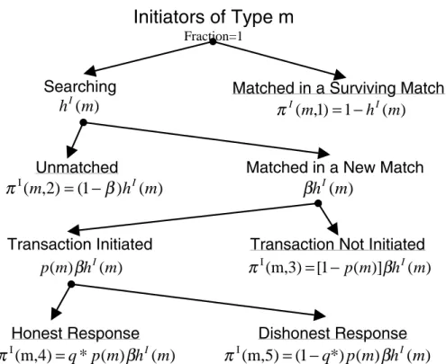
if an initiated transaction is met with a dishonest response, there is no net output produced (the theft is just a transfer). The extensive form of the transaction game is pictured in Figure 1.
This setup tries to capture the distinction between trust and trustworthiness and the impact both of these have on individual prosperity. Successful completion of a transaction requires both a trusting approach of the initiator and a trustworthy ap-proach of the respondent.4 In case either of them is missing, the transaction fails and
no net output is produced (although some existing wealth might be redistributed). Each period a subgroup of initiators interacts with a subgroup of respondents by 2The assumptions ofF andGbeing strictly increasing on the two supports are only made for presentational convenience. None of the results is affected by dropping this assumption.
3Note that we do not assume that d andm are distributed independently across individuals. Indeed, they may be correlated. Whether they are correlated or not, however, is immaterial to the subsequent analysis since each individual acts independently in his initiator and respondent roles.
Initiate the Transaction Do Not Initiate the Transaction Honest Response Dishonest Response
FIGURE 1: Extensive form of the transaction game
participating in an initiator-respondent match. Even though each individual has a dual role in each period, acting both as an initiator in one match and a respondent in another, it is helpful to separate these two roles and to think of the initiators and the respondents as two separate groups of the same size.5 At the beginning of each
period there are equally sized groups of matched initiators and matched respondents and equally sized groups of unmatched initiators and unmatched respondents. Those matched participate in their ”surviving” matches from the previous period. Each unmatched initiator gets matched with probability β ∈ (0,1) to some unmatched respondent and vice versa. Then, by the law of large numbers, β is also the fraction of both the searching initiators and the searching respondents who get matched in a new match within a period. If an initiator or a respondent is unmatched, 5This simplification is valid since the two matches of an individual (one in the initiator role and one in the respondent role) are generically different (their coincidence is a zero probability event).
his or her payoff for the current period is 0. If an initiator and a respondent are matched (in a new or a surviving match), they play the transaction game outlined above and collect their payoffs. If the transaction is completed successfully (i.e. it is initiated and responded to honestly), the match survives to the next period with probability α ∈ (0,1). Otherwise it is dissolved and both participants will enter the next period as unmatched. The latter is also the case if the transaction is completed successfully but, conditional on that, the match does not survive until the next period for exogenous reasons, which happens with probability 1−α. In turn,αis then also the fraction of matches with successfully completed transactions that actually survive to the next period. Intuitively, even if the match is ”working”, exogenous events such as population mobility or business turnover may cause the match to break up. All individuals are risk neutral and have a discount factor δ ∈ (0,1). We assume that α > β, i.e., that a working match is more likely to survive than a search is to result in a new match.
To make the analysis tractable, we restrict our attention to steady states and make the following additional assumptions.
Assumption 1: All the disclosed or inferred information about a partner in a transaction is specific to and lasts only during a given repeated match (i.e., there is no social learning and no memory).
Assumption 2: Both the initiators and the respondents condition their strate-gies only on what happened within the current period, on whether the present match is new or surviving and on the aggregate steady state probability of an initiator
ini-tiating (p) and a respondent responding honestly (q) in a new match.6
Assumption 3:If an initiator or a respondent is indifferent between two actions, she or he chooses to initiate or respond honestly, respectively.
In the next subsection, p and q are taken as given and the implied behavior of individual initiators and respondents is derived. The following subsection then aggregates these individual decisions to determine p and q endogenously.
2.2
Partial Equilibrium
At the beginning of a period, after both the initiators and the respondents have realized whether they are matched or not and whether the match is new or surviving, an initiator (of type)mmay find herself in the following states with their associated discounted payoff values (or value functions):
I1: Not matched: I1(m, q)
I2: Matched in a new match: I2(m, q)
I3: Matched in a surviving match: I3(m, q)
The value of q enters into the decisionmaking and value functions of initiators 6This Markovian strategy assumption is made in order to simplify the analysis. Given that a necessary condition for a match survival is a successful completion of the transaction in each period while the match lasts, a general strategy space would allow strategies to condition on the age of the match, since that is the only variable that may differ from one surviving match to another. Indeed, one could envision an equilibrium in which, conditional on match survival, initiators of type m
initiate until periodx(m) and respondents of typedrespond honestly until periody(d), wherex(·) and y(·) are (weakly) increasing and potentially infinitely valued. In such an equilibrium, given the age of a particular match, optimal initiator and respondent decisions would be determined by the intrinsic behavioral propensities and the updated distributions of match partner types (where the support of the latter only includes opponent types whose strategies prescribe cooperation until at least the realized age of the match). Intuitively, we focus on equilibria where x(·) and y(·) only assume values of zero or infinity. Although the general class of strategies and equilibria may be interesting from a purely theoretical standpoint, we believe that the subclass we focus on sufficiently captures the essentials of trust and trustworthiness in an equilibrium setting.
because it captures how likely one is to encounter an honest response in a new match.7
Based on the realization of whether he is matched or not, whether the match is new or surviving and whether the initiator has initiated a transaction or not, a respondent (of type)dmay find himself in the following states with their associated discounted payoff values (or value functions):
R1: Not matched: R1(d, p)
R2: Matched in a new match, but without an initiated transaction: R2(d, p)
R3: Matched in a new match with an initiated transaction: R3(d, p)
R4: Matched in a surviving match, but without an initiated transaction: R4(d, p)
R5: Matched in a surviving match with an initiated transaction: R5(d, p)
The value of p enters into the decisionmaking and value functions of initiators because it captures how likely one is to encounter a trusting initiator in a new match.8
First, consider the decisionmaking of a respondent d given p (for simplicity of notation, we omit p from the list of arguments in the value functions). In states R1, R2 or R4, there is no current decision to be taken and the respondent simply collects a payoff 0 in the current period. Then he goes searching at the beginning of the next period, since any existing match is dissolved at the end of the current 7The value of pdoes not enter into the initiators’ decisionmaking because it only matters to them to the extent it affects q. Hence q is a sufficient statistic from the point of view of the initiators.
8The value of q does not enter into the respondents’ decisionmaking because it only matters to them to the extent it affects p. Hencepis a sufficient statistic from the point of view of the respondents.
period. This implies that
R1(d) = R2(d) = R4(d) (1)
In addition to getting the payoff 0 in the current period, in the next period the respondent gets matched in a new match with probability β and, conditional on the latter, he will face an initiated transaction with probability p. Therefore the Bellman equation for R1(d) is
R1(d) = 0 +δ[(1−β)R1(d) +β(1−p)R2(d) +βpR3(d)] (2)
Using (1), this gives
R1(d) =R2(d) =R4(d) =
βδp
1−δ+βδpR3(d) (3)
If in state R3 or R5, the respondent must decide whether to respond to the initiated transaction honestly or dishonestly. If responding dishonestly, he collects 1−d in the current period and goes searching at the beginning of the next period. This is quantitatively equivalent to collecting 1−dcurrently and being in state R1 currently. If responding honestly, with probability 1−α the respondent collects a in the current period and the match dissolves, in which case the respondent goes searching at the beginning of the next period. This is quantitatively equivalent to collecting a currently and being in state R1 currently. With probability α the respondent collectsa in the current period and the match survives.
respondent has to form a belief about the initiator initiating in the next period in such scenario. This poses no complication if the current state is R5 because of the conditioning states used by the initiator in formulating her strategies (Assumption 2). In particular, the initiator will initiate again in the next period because she has done so in the current period. In other words, the fact that the initiator initiated in the current period perfectly reveals what action her strategy prescribes for surviving matches. Hence, in state R5 and conditional on the survival of the match, the respondent will again find himself in state R5 in the next period. Therefore the Bellman equation for R5(d) is
R5(d) = max{1−d+R1(d); (1−α) [a+R1(d)] +α[a+δR5(d)]} (4)
The first term in the maximand corresponds to the value of responding dishonestly while the second term corresponds to the value of responding honestly.
Analyzing (4) gives the following result:
Lemma 1 All the respondents (irrespective of d) respond honestly in state R5.
Intuitively, if in state R5, the respondent must have chosen to respond honestly in the previous period (in state R3) even in the presence of uncertainty about whether the initiator would or would not initiate in the current period. It then follows that the respondent will also opt to respond honestly once it is certain that the initiator will initiate in the next period.
This lemma and (4) then imply that
R5(d) = (1−α) [a+R1(d)] +α[a+δR5(d)]
which gives, by using (3),
R5(d) =
a 1−αδ +
(1−α)βδp
(1−αδ)(1−δ+βδp)R3(d) (5)
If in state R3, however, it is not obvious from the fact that the initiator has initiated in the current period that she will do so also in the next period (if the match survives until then) because the initiator’s strategy may prescribe different actions for states I2 and I3. Hence let k ∈ [0,1] be the belief of the respondent that the initiator will initiate in the next period if the match survives till then. Because k is defined conditionally on the initiator initiating and the respondent responding honestly in the current period, its value is, on the same conditioning set, independent of d and m that characterize the two participants to the current match. This is because, in the next period, the initiator will only observe that the match has survived, if it does, not a particular value of d. Similarly, when forming his belief, the respondent only observes that the transaction has been initiated in the current period, not a particular value of m. If the initiator does not initiate, the respondent will get to state R4. In the opposite case the respondent will get to
state R5. Then, in analogy with (4),
R3(d) = max{1−d+R1(d); (1−α) [a+R1(d)] +α[a+ (1−k)δR4(d) +kδR5(d)]}
(6) Again, the first term in the maximand corresponds to the value of responding dis-honestly while the second term corresponds to the value of responding dis-honestly.
Before continuing the analysis of respondents’ actions in state R3, it is useful to consider the decisionmaking of the initiators. Hence consider the decisionmaking an initiator m given q (for simplicity of notation, omit q from the list of arguments in the value functions). If in state I1, there is no current decision to be taken and the initiator simply collects a payoff 0 in the current period. In the next period she gets matched in a new match, hence getting into state I2, with probability β and does not get matched, hence getting into state I1, with probability 1−β. Therefore the Bellman equation for I1(m) is
I1(m) = 0 +δ[(1−β)I1(m) +βI2(m)] (7)
giving
I1(m) =
βδ
1−δ+βδI2(m) (8)
If in states I2 or I3, the initiator must decide whether to initiate a transaction or not. If not initiating, she collects−m in the current period and goes searching at the beginning of the next period. This is quantitatively equivalent to collecting −m currently and being in state 1 currently. If in state I3 and initiating, it follows by
Lemma 1 that the respondent will respond honestly. Then with probability 1−αthe initiator collects a in the current period and the match dissolves, in which case the initiator goes searching at the beginning of the next period. This is quantitatively equivalent to collectingacurrently and being in state I1 currently. With probability αthe initiator collects ain the current period and the match survives, in which case the respondent will be in state I3 in the next period. Therefore the Bellman equation for I3(m) is
I3(m) = max{−m+I1(m); (1−α) [a+I1(m)] +α[a+δI3(m)]} (9)
The first term in the maximand corresponds to the value of not initiating while the second term corresponds to the value of initiating.
If in state I2 and initiating, however, it is not certain that the respondent will re-spond honestly. In particular, since the matching process is random, the probability of the respondent responding honestly is q. If the respondent responds dishonestly, the initiator will collect−1 in the current period and will go searching at the begin-ning of the next period. This is quantitatively equivalent to collecting−1 currently and being in state I1 currently. If the respondent responds honestly, reasoning analogous to state I3 applies. Therefore
I2(m) = max{−m+I1(m); (1−q) [−1 +I1(m)] (10)
Again, the first term in the maximand corresponds to the value of not initiating, while the second term corresponds to the value of initiating.
Lemma 2 All the initiators (irrespective of m) initiate in state I3.
Intuitively, if in state I3, the initiator must have chosen to initiate in the previous period (in state I2) even in the presence of uncertainty about whether the respondent would respond honestly or dishonestly. Consequently, the initiator will also initiate once it is certain that the respondent will respond honestly.
This lemma and (9) then imply that
I3(m) = (1−α) [a+I1(m)] +α[a+δI3(m)]
which gives, by using (8),
I3(m) =
a 1−αδ +
(1−α)βδ
(1−αδ)(1−δ+βδ)I2(m) (11)
Note the importance of Lemma 1 and Lemma 2: they imply that a successful completion of the transaction in the initial period of a match is a sufficient signal for both sides for developing trust and trustworthiness between them. This manifests itself in successful completion of the transaction in every subsequent period for as long as the match lasts.9
Now we can finalize the partial equilibrium analysis. Using the result of Lemma 2,k, which is the belief of the respondent in state R3 that the initiator will initiate 9Once trust and trustworthiness have been established, the expected survival time of a match is α
in the next period if the match survives until then, becomes 1 in (6). The latter, combined with (3) and (5), then gives
R3(d) = max ½ 1−δ+βδp 1−δ (1−d); 1−δ+βδp (1−δ)(1−αδ)a− αβδp 1−αδR3(d) ¾ (12)
where, as before, the first term in the maximand corresponds to the value of re-sponding dishonestly, while the second term corresponds to the value of rere-sponding honestly.
Lemma 3 A respondent d responds honestly in state R3 if and only if d ≥d(p)≡
1− a
1−αδ+αβδp.
This result is a straightforward implication of (12) and Assumption 3 and its proof is left to the reader.
Lemma 3 says that, in a new match, respondents with a relatively high level of intrinsic honesty will behave in a trustworthy way and reply honestly, while respondents with a relatively low intrinsic honesty will not behave in a trustworthy way and they will reply dishonestly. This is so because the latter group will find theft attractive because of their low ”moral barriers”, even though it entails termination of the match. On the other hand, the former group will not find theft attractive either because of their high ”moral barriers” or because of reputation reasons, since it is more profitable for them to continue the match, even though they would behave dishonestly in a non-repeated setting. The threshold d(p) is an increasing function ofp, the aggregate steady state probability of an initiator initiating in a new match. Note that this implies that trust breeds untrustworthiness. The more trusting the
population, the more attractive acting in an untrustworthy way is. This is because the more likely the initiators are to trust strangers, the easier it is to get into state R3 (new match with an initiated transaction) if unmatched at the beginning of a period, and hence the less costly it is to forego reputation (and hence break up the match) by stealing relative to the gain from stealing, which is unchanged. Consequently, more respondents will choose to respond dishonestly in a new match with an initiated transaction. Note, however, that respondents with d ≥ 1 never choose to behave dishonestly.
In a similar way, using (8) and (11) for substitution into (10) yields
I2(m) = max ½ −1−δ+βδ 1−δ m; (q+aq−1 +αδ−αδq)(1−δ+βδ) (1−δ)(1−αδ) − αβδq 1−αδI2(m) ¾ (13) where, as before, the first term in the maximand corresponds to the value of not initiating, while the second term corresponds to the value of initiating.
Lemma 4 An initiator m initiates the transaction in state I2 if and only if m ≥
m(q)≡ (1−q1−αδ)(1−αδ+αβδq)−aq.
Again, this result is a straightforward implication of (13) and Assumption 3 and its proof is omitted.
Lemma 4 says that, in a new match, initiators with a relatively high level of intrinsic trust will behave in a trusting way and initiate, while initiators with a relatively low intrinsic trust will not trust and thus will not initiate. The threshold m(q) is a decreasing function of q, the aggregate steady state probability of a re-spondent responding honestly in a new match. This is intuitive. The more likely the
respondents are to behave honestly in a new match, the more initiators will choose to trust them. In particular, a higher value of q implies a decreased likelihood of theft and an increased likelihood of a mutually profitable long-term relationship.
Lemmata 1through 4 completely characterize initiator and respondent behavior in all states where they need to make a decision. They relate this behavior to aggregate measures of trusting (p) and trustworthy (q) behavior in new matches. Of course, the latter are not exogenous and should themselves be treated as aggregates of individual behavior. The next section turns to this task.
2.3
General Equilibrium Analysis
This section builds on Lemmata 1 through 4 in characterizing the general equi-librium in the society. The central idea is simple: an equiequi-librium is a pair (p, q) that is mutually consistent under the initiator-respondent interactions. To elaborate in more detail, consider a particular value of p and how this value maps to a value of q consistent with it. By Lemma 3, the respondents with d ≥d(p) respond hon-estly if called to respond in a new match, while the others respond dishonhon-estly. To simplify the language, call the former ones ”trustworthy” and call the latter ones ”untrustworthy”. It follows that the measure of trustworthy respondents is Q ≡
1−F [d(p)] and the measure of untrustworthy respondents is 1−Q = F [d(p)].10 10To clarify the notation, note that q is the conditional steady state probability measure of trustworthy respondents, where the conditioning is based on the set of searching respondents. When multiplied by the steady state measure of searching respondents, it gives the measure of searching respondents whostand readyto behave in a trustworthy way in the current period (or any other specific period). On the other hand,Qis theunconditional steady state probability measure of trustworthy respondents. That is, it is the measure of respondents who would behave in a trustworthy way if they happened to find themselves in a new match with an initiated transaction in the current period (or any other specific period).
Sinceqis the aggregate steady state probability of a respondent responding honestly in a new match, it must be equal to the fraction of trustworthy searching respon-dents among the searching responrespon-dents. Because all the untrustworthy responrespon-dents search at the beginning of each period (since they never participate in a surviving match), we only need to find the fraction of trustworthy respondents that search in order to deduce q. Denote the latter fraction hR. Since this fraction has to stay
constant over time in a steady state, in any period the measure of new matches involving trustworthy respondents that survive until the following period has to be equal to the measure of surviving matches involving trustworthy respondents that get dissolved in the current period. As for the former, the fraction hR of
trustwor-thy respondents that search results in the fraction βhR of trustworthy respondents
involved in new matches, the fraction pβhR of trustworthy respondents involved in
new matches experiencing an initiated transaction, the fractionpβhRof trustworthy
respondents involved in new matches experiencing a successfully completed trans-action and, finally, the frtrans-action αpβhR of trustworthy respondents involved in new
matches that survive until the following period. As for the latter, the fraction 1−hR
of trustworthy respondents participating in surviving matches results in the fraction (1−α)(1−hR) of trustworthy respondents participating in surviving matches that
get dissolved in the current period. In equilibrium, then, αpβhR= (1−α)(1−hR),
which gives
hR = 1−α
Consequently, the measure of searching respondents isF [d(p)]+ 1−α
1−α+αβp{1−F [d(p)]}. The previous analysis then implies that the value of q that is consistent with p is given by q =T(p), where T : [0,1]−→[0,1] is defined by
T(p)≡ 1−α 1−α+αβq{1−F [d(p)]} F [d(p)] + 1−α 1−α+αβq{1−F [d(p)]} = (1−α){1−F [d(p)]} 1−α+αβpF [d(p)] (15) ∀p∈[0,1].
Now consider a particular value of q and how this value maps to a value of p consistent with it. By Lemma 4, the initiators with m ≥ m(q) initiate in a new match, while the others do not. Call the former ones ”trusting” and the latter ones ”mistrusting”. It follows that the measure of trusting initiators is P ≡ 1−
G[m(q)] and the measure of mistrusting initiators is 1−P =G[m(q)].11 Sincep is
the aggregate steady state probability of an initiator initiating in a new match, it must be equal to the fraction of trusting searching initiators among the searching initiators. Because all the mistrusting initiators search at the beginning of each period (since they never participate in a surviving match), we only need to find the fraction of trusting initiators that search in order to deducep. Denote the latter hI.
Then, following a similar logic as above, we get that
hI = 1−α
1−α+αβq (16)
11Again, to clarify the notation, note thatpis theconditional steady state probability measure of trusting initiators, where the conditioning is based on the set of searching initiators. When multiplied by the steady state measure of searching initiators, it gives the measure of searching initiators whoactuallybehave in a trusting way in the current period (or any other specific period). On the other hand,P is theunconditional steady state probability measure of trusting initiators. That is, it is the measure of initiators who would behave in a trusting way if they happened to find themselves in a new match in the current period (or any other specific period).
Consequently, the measure of searching initiators isG[m(q)]+ 1−α
1−α+αβq{1−G[m(q)]}. The previous analysis then implies that a value ofpthat is consistent withqis given byp=V(q), where V : [0,1]−→[0,1] is defined by V(q)≡ 1−α 1−α+αβq{1−G[m(q)]} G[m(q)] + 1−α 1−α+αβq{1−G[m(q)]} = (1−α){1−G[m(q)]} 1−α+αβqG[m(q)] (17) ∀q∈[0,1].
We now define a general equilibrium formally:
Definition 1 Ageneral trust/trustworthiness equilibrium is a pair (p∗, q∗)∈[0,1]2 that satisfies p∗ =V(q∗) and q∗ =T(p∗).1213
12A reader may wonder why we do not impose an additional equilibrium condition requiring that the measure of searching initiators be equal to the measure of searching respondents, i.e., that
G[m(q∗)] + 1−α
1−α+αβq∗{1−G[m(q
∗)]}=F[d(p∗)] + 1−α
1−α+αβp∗{1−F[d(p
∗)]} (18)
However, this additional requirement is redundant since this equality is guaranteed for any existing equilibrium. To see that, the two equilibrium conditions imply that
G[m(q∗)] = (1−p∗)(1−α)
1−α+αβp∗q∗ (19)
and
F[d(p∗)] = (1−q∗)(1−α)
1−α+αβp∗q∗ (20)
Using these results, both sides of the (18) are equal to
h= 1−α
1−α+αβp∗q∗ (21)
wherehdenotes a common measure of searching initiators and respondents in an equilibrium. 13Given a particular general equilibrium (p∗, q∗)of aggregate steady state probabilities of
initia-tors initiating and respondents responding honestly in a new match, one can deduce the equilibrium measures of trusting initiators and trustworthy respondents, that is P∗ andQ∗, by
P∗= 1−G[m(q∗)] (22)
and
The next theorem establishes existence of a general equilibrium.
Theorem 1 There exists a general trust/trustworthiness equilibrium.
Although existence can be established by a routine argument, uniqueness is not guaranteed by the previous assumptions. To see this, note that because d(.) is increasing, T is decreasing. However, although m(.) is decreasing, an increasing property ofV cannot be deduced. Intuitively, an increase inphas two effects. First, the trustworthiness threshold d(p) increases and hence there will be less trustwor-thy and more untrustwortrustwor-thy respondents in the overall population of respondents. Second, as can be seen from (14), a lower fraction of trustworthy respondents will be searching. Ceteris paribus, each effect tends to reduce the share of trustworthy searching respondents among the searching respondents. That is, both effects work in the same direction and T(p) decreases as a result. Similarly, an increase in q has two effects. First, the trust threshold m(q) decreases and hence there will be more trusting and less mistrusting initiators in the overall population of initiators. Second, as can be seen from (16), a lower fraction of trusting initiators will be searching. Ceteris paribus, the first effect tends to increase the share of trusting searching initiators among the searching initiators, while the second effect has just the opposite impact. Hence the two effects work in opposite directions, and it is not in general possible to say which one will prevail.14 Figure 2 illustrates a case when
bothT and V are monotone, which results in a unique general equilibrium.
14Facing a possibility of multiple equilibria, one may wonder whether there would be a convenient sufficient condition that would rule such case out. (19) and (20) imply that
q
p 0 q* 1 1 * p)
(q
V
)
(
1q
T
−FIGURE 2: Illustration of general equilibrium
3
Empirical Predictions for Individual Prosperity
We are interested in how individual prosperity depends on whether one trusts or not and on whether one is or is not trustworthy. To be able to do that, we need to pick a measure of prosperity. Because the inherent utility of honesty and the inherent utility of trust are unobservable, our primary measure of individual prosperity is an expected, or average, payoff in a single period, net of either type of inherent utility.Conceptually, there is a particular steady state equilibrium in the background. in any general equilibrium. Suppose there are at least two equilibria. Then (24) has to be satisfied for at least two different equilibrium pairs (p∗
1, q∗1) and (p∗2, q2∗), where, without loss of generality,
p∗
1 < p∗2. Since T is strictly decreasing, it must also be the case that q∗1 > q∗2. Now consider a shift from the first to the second equilibrium. Because m(.) is decreasing, the right-hand side of (24) increases and hence so must the left-hand side to preserve the equality. Therefore a convenient sufficient condition to rule out multiplicity of equilibria is to require that (1−p)F[d(p)] is nonincreasing inp. However, we do not wish to impose this assumption since it is not essential for our objectives.
In that equilibrium, an individual, be it an initiator or a respondent, may find herself or himself in five different outcomes at the end of a typical period.15 First, (s)he may
be matched in a surviving match. Second, (s)he may be unmatched. Third, (s)he may be matched in a new match without an initiated transaction. Fourth, (s)he may be matched in a new match with an initiated transaction and an honest response. Fifth, (s)he may be matched in a new match with an initiated transaction, but with a dishonest response. Let the steady state probabilities of these five outcomes be, in the same order, πI(m, i) and πR(d, i), i∈ {1,2,3,4,5}, for initiators of type m and
respondents of type d, respectively. The per period payoffs for both the initiators and the respondents are a in outcome 1 and 4, 0 in outcome 2 and 3, and they are
−1 for the initiators and 1 for the respondents in outcome 5. Hence the expected payoff ΠI(m) for an initiator of type m is
ΠI(m) =£πI(m,1) +πI(m,4)¤a−πI(m,5) (25)
and the expected payoff ΠR(d) for a respondent of typed is
ΠR(d) = £πR(d,1) +πR(d,4)¤a+πR(d,5) (26)
In order to be able to compute these expected payoffs, we need to find the steady state equilibrium probability distribution over the five outcomes for each initiator and for each respondent. This is the task to which we turn now.
15Note that the concept of outcome is different from the concept of state. While states are various ex ante decisionmaking situations, outcomes are various ex post payoff situations.
The first step in this process involves finding the fraction (or conditional mea-sure) of initiators and the fraction of respondents of each type who search at the beginning of a generic period. Given the latter, the probability distribution over the individual outcomes for each type can be computed using the exogenous match-ing probability β together with an equilibrium degree of trusting and trustworthy behavior, both on the aggregate and the individual level. As in the previous sec-tion, one only needs to distinguish between trusting and mistrusting initiators and trustworthy and untrustworthy respondents, since behavior is uniform within each of these groups. Letp: [0,1]→[0,1] be a function that maps initiator types to equi-librium probabilities of (initiators of that type) initiating if having an opportunity. By Lemma 6, p(m)≡ 1 if m≥m(q∗) (trusting initiators) 0 otherwise (mistrusting initiators)
(27)
Also let q : [0,1] −→ [0,1] be a function that maps respondent types to equilib-rium probabilities of (respondents of that type) responding honestly to an initiated transaction. By Lemma 5, q(d)≡ 1 if d≥d(p∗) (trustworthy respondents) 0 otherwise (untrustworthy respondents)
(28)
Now lethI : [0,1]−→[0,1] be a function that maps initiator types to equilibrium
let hR : [0,1] −→ [0,1] be a function that maps respondent types to equilibrium
fractions (of respondents of that type) that search at the beginning of each period. Then, using the results of the previous section, we get that
hI(m) = 1−α 1−α+αβq∗ if m ≥m(q∗) (trusting initiators)
1 otherwise (mistrusting initiators)
(29) and hR(d) = 1−α 1−α+αβp∗ if d≥d(p∗) (trustworthy respondents)
1 otherwise (untrustworthy respondents)
(30)
Given the functional forms ofpI,pR,hI andhR, Figures 3 and 4 depict the
prob-ability distribution over the five outcomes for initiators of type m and respondents of typed, respectively.
Combining (25), (26) and the information from Figure 3 and Figure 4 then gives
ΠI(m) =£1−hI(m) +q∗p(m)βhI(m)¤a−(1−q∗)p(m)βhI(m) (31)
and
ΠR(d) =£1−hR(d) +q(d)p∗βhR(d)¤a+ [1−q(d)]p∗βhR(d) (32)
Finally, after using (27), (28), (29) and (30) to substitute into (31) and (32), the expected per period payoff for a trusting initiator is
Fraction=1 ) (m hI πI(m,1)=1−hI(m) ) ( ) 1 ( ) 2 , ( I m h m
β
Iπ
= −β
h
I(
m
)
) ( ) (m h m p β I πI(m,3)=[1− p(m)]βhI(m) ) ( ) ( * (m,4) I m h m p qβ
Iπ
=π
I(m,5)=(1−q*)p(m)β
hI(m)FIGURE 3: Probability distribution over outcomes for initiators of type m
Fraction=1 ) (d hR πR(d,1)=1−hR(d) ) ( ) 1 ( ) 2 , ( R d
β
hR dπ
= −β
h
R(
d
)
) ( * h d p β R πR(d,3)=(1− p*)βhR(d) ) ( * ) ( (d,4) R q d pβ
hR dπ
=π
R(d,5)=[1−q(d)]p*β
hR(d)ΠI
trusting =
β[q∗a−(1−q∗)(1−α)]
1−α+αβq∗ , (33)
the expected per period payoff for a mistrusting initiator is
ΠI
mistrusting = 0, (34)
the expected per period payoff for a trustworthy respondent is
ΠR
trustworthy =
βp∗
1−α+αβp∗a, (35)
and the expected per period payoff for an untrustworthy respondent is
ΠRuntrustworthy =βp∗. (36)
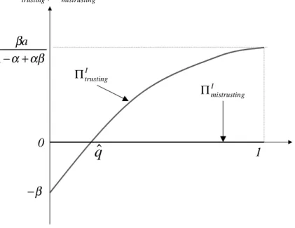
In general, ΠI
trusting may be more or less than ΠImistrusting, depending on the value of the parameters and the shapes of F and G. So it is not possible to con-clude in general whether trust does or does not increase expected income (i.e., ”pay off”). However, for q∗ = 0 we have ΠI
trusting = −β < ΠImistrusting, for q∗ = 1 we have ΠI
trusting = βa/(1−α +αβ) > ΠImistrusting, and ΠItrusting is continuous and strictly increasing in q∗. Therefore we can conclude that trust does not pay off in low trustworthiness societies, but it does pay off in high trustworthiness societies. Furthermore, it pays off more the more trustworthy a society is. The threshold value of q∗ that makes the two payoffs equal is qb≡ 1−α
*
q
I g mistrustin I trusting Π Π , 0 1qˆ
αβ α β + − 1 a β − I trusting Π I g mistrustin ΠFIGURE 5: Expected equilibrium payoffs of trusting and mistrusting initiators as functions of q∗
and it does not pay off if q∗ <q. This is illustrated in Figure 5.b Similarly, ΠR
trustworthy may be more or less than ΠRuntrustworthy and hence it is not possible to conclude in general whether trustworthiness does or does not pay off. For p∗ = 0 we have ΠR
trustworthy = ΠRuntrustworthy. Since ΠRtrustworthy is strictly increasing and strictly concave in p∗, three scenarios, depicted in Figure 6, are possible. First, if a ≥ 1−α+αβ, the ”high” case, trustworthiness pays off no matter what the social level of trust p∗ is. Second, if 1−α+αβ > a > 1−α, the ”medium” case, trustworthiness pays off for low levels of social trust, in particularp∗ ≤pb≡ a−(1−α)
αβ , but it does not pay off for high levels of social trust, i.e. when p∗ > p. Third, ifb 1−α > a, the ”low” case, trustworthiness does not pay off for any level of social trust.
*
p
thy untrustwor R y trustworth R Π Π , 0 1 (high) y trustworth R Π (low) y trustworth R Π (medium) y trustworth R Π thy untrustwor R Π pˆFIGURE 6: Payoffs of trustworthy and untrustworthy respondents as functions of p∗
aspects of countries that determine the equilibrium values of p∗ and q∗ - the distri-butions G(.) and F(.) of inherent attitudes, and the values of α, β, δ and a—also affect the difference in expected income between trusting and not trusting for any given level ofq∗, and between being and not being trustworthy for any given level of p∗. For this reason, one cannot interpret Figures 5 and 6 as directly revealing how the expected difference in income depends on the values of p∗ and q∗. Many of the variations in fundamentals that affect p∗ andq∗ will also affect the expected income of a person conditional on their attitude.
This stylized model of how individual attitudes combine to generate an equilib-rium provides the framework we use in the empirical analysis of whether trust and trustworthiness pay off that we develop in Sections 5 and 6. In particular, we will
examine the model’s prediction that the payoff to exhibiting each of these behav-iors depends on the aggregate prevalence of the complementary attitude. Before we begin the empirical analysis, though, we briefly review the empirical literature that is related to our investigation.
4
Empirical Literature Review
16There is some empirical evidence that trust and civic duty among a country’s citizens contribute to growth. Knack and Keefer (1997) tested the impact of these attitudes on both growth and investment rates in a cross-section of 29 countries, using measures of trust and civic norms from the World Values Surveys of 1981 and 1990. They find that social capital variables exhibit a strong and significant positive relationship to economic growth. As they note, the causality of this relationship could go in either direction: trust could be a product of optimism generated by high or growing incomes, or it could be that trust facilitates prosperity. However, they find that trust is more correlated with per capita income in later years than with income in earlier years, suggesting that the causation runs from trust to growth more so than vice versa.
Zak and Knack (2001) extend the Knack and Keefer framework by separately testing for the effect on growth of proxies for the presence of formal institutions, social distance, and discrimination and for whether their effect remains significantly 16In this review, we focus on the impact of trust and trustworthiness on economic
outcomes. There is also literature studying the determinants of trust. See Alesina and Ferrara (2000) for a recent contribution.
correlated with growth controlling for measures of trust. They find that trust is positively and significantly related to growth even in the presence of measures of formal institutions or of social distance, but that most of the influence of the latter on growth occurs through their impact on trust. The one exception is a measure of property rights, which retains its independent positive association with growth even in the presence of a trust variable. They justify this finding by noting that this index includes government actions against private agents. In contrast, the trust measure is “likely to be little affected by perceptions of the trustworthiness of government. . . ” (p. 316)
La Porta, Lopez-de-Silvanes, Shleifer, and Vishny (1999) find that, across coun-tries, a one-standard deviation increase in the measure of trust increases judicial efficiency by 0.7 of a standard deviation and reduces government corruption by 0.3 of a standard deviation. Putnam (1993) examines cross-regional Italian data and concludes that local governments are more efficient where there is greater civic engagement.
In what follows, we use a somewhat different empirical strategy by examining household-level rather than country-level data from 18 countries. In particular, we estimate regression equations explaining household income with a specification that is based on the standard earnings equations from labor economics, but that is augmented to test for the impact of trust, trustworthiness and their interaction with aggregate levels of the complementary attitude. The theoretical model of Sections 2 and 3 frames our approach.
5
Data
Although the theory provides a consistent framework in which to evaluate data, it leaves open the precise relationship between income and personal and country characteristics. To shed empirical light on the issues discussed in the previous section, one needs measures of individual well-being, personal trust, trustworthiness and, preferably, some additional sociodemographic variables. To our knowledge, only two datasets provide this information: the National Opinion Research Center’s General Social Survey (GSS) and the World Values Survey (WVS). In order to identify the impact of aggregate trust and trustworthiness within the society, we must use WVS, as it, unlike the GSS, provides individual-level data for multiple countries.
The purpose of the WVS is to facilitate cross-national comparisons of values, norms, and attitudes. The survey was conducted in multiple waves, with limited national modifications, in several dozen countries. It asked about attitudes concern-ing work, family, religion, politics, and contemporary social issues and gathered a limited amount of demographic data as well. Although the data are subject to the usual reservations about attitude surveys, and in particular cross-country attitude surveys, the data has been widely and fruitfully used by political scientists and so-ciologists, not to mention Knack and Keefer (1997) and Zak and Knack (2001). For an extensive, albeit incomplete, list of its use in research, see Inglehart, Basanez, and Moreno (1998). We use the data from the 1990-93 wave for 18 developed and
developing countries.17 We excluded the former communist countries because their
economic and incentive structure as of the time of the survey was not conducive to trust and trustworthiness having much effect on individual prosperity.18 We
supple-ment the WVS data with Summers and Heston (1991) Penn World Tables (PWT), Mark 5.6 to be able to make real income comparisons across countries.
Our measure of trust is based on the following WVS question: ”Generally speak-ing, would you say that most people can be trusted or that you can’t be too careful in dealing with people?” This question offered two responses: ”can’t be too careful” and ”most people can be trusted”. We associate the former answer with ”mis-trusting” individuals and the latter answer with ””mis-trusting” individuals. Based on these survey responses, we create a binary variable TRUST indicating the trusting individuals. Our measure of trustworthiness is based on the following WVS ques-tion: ”Please tell me whether you think lying in your own interest can always be justified, never be justified, or something in between.” This question offered 10 re-sponses ordered from 1 (never justified) to 10 (always justified). In order to measure trustworthiness, we reversed the scale and call the resulting variable TRUSTW.
Glaeser et al. (2000) measure trust and trustworthiness by conducting experi-ments with monetary rewards. They find that the standard question used to measure 17We use the following countries: Austria, Belgium, Brazil, Britain, Canada, Chile, Finland, India, Italy, Japan, Mexico, The Netherlands, Portugal, South Africa, Spain, Turkey, USA, and West Germany.
18As for the remaining countries in the 1990-93 wave, we could not use Argentina, Denmark, Ireland, Nigeria, Norway, Sweeden, and Switzerland because the income category thresholds that we use for measuring real household income (see below) were not available. We could not use France because the household income data records did not precisely match with the available income category thresholds. We could not use Iceland because of the missing household income data. Finally, we could not use South Korea because of the missing education data.
trusting behavior - used in the WVS as well as the GSS - does not have a significant correlation with trusting choices in either of two experiments. Two other questions, specifically about trusting strangers, do, though, predict trust (of strangers, in their experiments). Furthermore, the answers to questions about trustworthiness are not significantly related to trustworthy behavior. Surprisingly, a self-reported trusting attitude does appear to predict trustworthy behavior. Danielson and Holm (2002) conduct a similar experiment in Tanzania. They confirm that the standard survey question used to measure trust does not predict actual trusting behavior in their ex-perimental setting. Unlike Glaeser et al. (2000), though, they find that the specific trust questions do not predict actual trusting behavior and that the general trust question does not predict trustworthy behavior. They also find that self-reported trustworthiness does in fact predict trustworthy behavior, but this effect disappears when donation motives are controlled for.
Glaeser et al. (2000) and Danielson and Holm (2002) conclude that empirical work based on the WVS/GSS survey questions about trust needs to be reinterpreted. While we take seriously the possibility that self-reported attitudes and behavior may not be highly correlated, we do find below that these self-reports help explain individual incomes with a systematic pattern, and so we conclude that they do reflect individual behavior in an important sense. Finally, although experimental evidence could certainly extend our knowledge of these issues, we expect that such evidence will not be available across countries in the near future, rendering the current study infeasible from this angle.
follow-ing WVS question: ”Here is the scale of incomes and we would like to know in what group your household is, counting all wages, salaries, pensions and other incomes that come in. Just give the letter of the group your household falls into, before taxes and other deductions.” This question offered 10 country-specific ranges for income. We convert the thresholds into 1990 purchasing power parity U.S. dollars using the PWT measure of PPP-based exchange rates. Our measure of real household income is a midpoint of each range and 150% of the highest threshold for the top range. Summary statistics for household income, trust and trustworthiness by country are reported in Table 1.
Because individual trust and trustworthiness are certainly not to be the only determinants of individual income, we examine additional sociodemographic infor-mation provided by WVS. Our measure of respondent education is based on the following WVS question: ”At what age did you or will you complete your full time education, either at school or at an institution of higher education? Please exclude apprenticeships.” This question offered a 10-point scale ranging from 1 (12 years of age or earlier) to 10 (21 years of age or older). In addition, we use the data on respondent age and gender. It is important to note that the measure of income we investigate relates to the household, but both the attitude indicators and sociode-mographic variables refer to the respondent. We will have more to say later about how that affects the interpretation of our results.
T ABLE 1: Summary statistics of real household income, trust and trust w orthiness by coun try HOUSEHOLD INCOME TR UST TR USTW OR THINESS COUNTR Y Obs. Mean Std. Dev. Obs. Mean Std. Dev. Obs. Mean Std. Dev. Austria 1414 18.28 11.65 1301 0.318 0.466 1440 8.27 2.04 Belgium 1705 21.14 13.29 2576 0.332 0.471 2730 7.04 2.62 Brazil 1679 6.36 9.69 1766 0.067 0.249 1774 8.20 2.73 Britain 1101 24.80 17.47 1440 0.436 0.496 1473 8.17 2.08 Canada 1461 35.88 23.50 1673 0.524 0.500 1712 8.18 2.24 Chile 1470 6.74 7.22 1458 0.227 0.419 1495 8.65 2.23 Finland 586 29.52 15.13 558 0.627 0.484 580 8.13 1.97 India 2429 4.77 3.87 2365 0.343 0.475 2480 8.76 2.03 Italy 1424 21.52 23.12 1932 0.371 0.483 1987 8.33 2.19 Japan 896 32.39 18.98 911 0.417 0.493 968 8.75 1.83 Mexico 1451 19.29 29.68 1384 0.335 0.472 1513 6.76 2.95 Netherlands 790 23.60 15.26 965 0.558 0.497 1010 7.49 2.11 P ortugal 1124 13.24 10.27 1149 0.214 0.410 1169 7.47 2.68 South Africa 2456 24.68 18.69 2594 0.283 0.450 2681 8.05 2.89 Spain 3431 11.19 8.04 3887 0.338 0.473 4042 8.07 2.32 T urk ey 1007 12.50 18.27 1012 0.100 0.300 1017 8.72 2.23 USA 1696 34.83 22.44 1782 0.500 0.500 1821 8.59 2.02 W est German y 1932 23.68 14.27 1725 0.378 0.485 2013 7.46 2.34 TOT AL 28052 20.24 19.28 30478 0.354 0.478 31905 8.06 2.40 Notes: All summary statistics are w eigh ted av erages based on surv ey w eigh ts pro vided with the data, with the sums of w eigh ts equalized across coun tries.
6
Empirical Results
6.1
Baseline Results
Table 2 reports our baseline results.19 It presents the results of regressing the
logarithm of real household income against variables that are standard in micro earn-ings equations plus indicators of the individual’s level of trust and trustworthiness, sometimes interacted with the mean level of these variables in the respondent’s coun-try. All of the regressions include country dummy variables (coefficients of which are not reported here), and so all the estimated coefficients are identified from within-country variation only. In all reported specifications, these within-country dummies are jointly significant at 1 percent level. The specification in Column (1) contains only the standard variables in an earnings equation. The results are in line with the empirical literature discussed above, lending credence to the survey-based measures of income, education, age, and gender. The marginal return to the respondent’s ed-ucation level is always positive within the observed range (between 6 and 15 years), although decreasing. Based on the estimated coefficients, going from zero to ten years of education adds 87 percent to income. Furthermore, the marginal return is 11.1 percent per year at 0 years, and falls to 6.29 percent at 10 years. These results are within the range reported in the literature , as discussed earlier.20 The respon-19The regressions are calculated using observations unweighted within countries and with sums of weights equalized across countries. We have also estimated analogous regressions without any (cross-country) weight adjustment and with weighting within and across countries combined. None of the principal results reported in this section are affected by this change.
20In the human capital earnings approach standard in labor economics, more recent estimates of the return to education fall anywhere between 0.023 (Isacsson (1999)) and 0.153 (Harmon and Walker (1995)) per additional year of schooling, depending on the dataset used, the set of control variables and the econometric technique. Card (1999) provides a good summary of this literature.
T ABLE 2: Regressions results: The impact of trust and trust w orthiness on real household income Dep enden t variable: Log of Real Household Income (1) (2) (3) (4) (5) (6) (7) Education 0.111 0.111 0.109 0.110 0.112 0.106 0.108 (0.0175)*** (0.0180)*** (0.0176)*** (0.0181)*** (0.0180)*** (0.0176)*** (0.0181)*** Education Squared 0.241 -0.247 -0.230 -0.244 -0.250 -0.217 -0.235 × 10 − 2 (0.0778)*** (0.0799)*** (0.0781)*** (0.0802)*** (0.0799)*** (0.0781)*** (0.0801)*** Age 0.368 0.362 0.374 0.370 0.361 0.375 0.370 × 10 − 1 (0.0192)*** (0.0198)*** (0.0193)*** (0.0199)*** (0.0198)*** (0.0193)*** (0.0199)*** Age Squared -0.474 -0.469 -0.477 -0.474 -0.469 -0.479 -0.475 × 10 − 3 (0.0204)*** (0.0211)*** (0.0206)*** (0.0212)*** (0.0211)*** (0.0205)*** (0.0212)*** Male 0.0837 0.0866 0.0822 0.0855 0.0870 0.0836 0.0874 (0.0108)*** (0.0111)*** (0.0109)*** (0.0111)*** (0.0111)*** (0.0109)*** (0.0111)*** T rust 0.0733 0.076 -0.448 -0.394 (0.0118)*** (0.0118)*** (0.197)** (0.198)** T rust w orthiness -0.117 -0.124 -0.362 -0.347 × 10 − 1 (0.0246)*** (0.0251)*** (0.0718)*** (0.0721)*** T rust*Av.T rust w orthiness 0.0647 0.0581 (0.0241)*** (0.0243)** T rust w orthiness*Av.T rust 0.0750 0.0685 (0.0193)*** (0.0192)*** Coun try Fixed Effects Y es Y es Y es Y es Y es Y es Y es Observ ations 26046 24544 25675 24235 24544 25675 24235 R-squared 0.42 0.42 0.42 0.43 0.42 0.42 0.43 Note 1: The regressions are calculated using observ ations un w eigh ted within coun tries and with the sums of w eigh ts equalized across coun tries. Note 2: Heteroscedasticit y consisten t robust standard errors are in paren theses. Significance lev el notation: ∗at 10%, ∗∗ at 5%, ∗∗∗ at 1%.