Cambridge Working Papers in Economics: 1968
A UNIT COMMITMENT AND ECONOMIC DISPATCH
MODEL OF THE GB ELECTRICITY MARKET –
FORMULATION AND APPLICATION TO HYDRO PUMPED
STORAGE
Chi Kong Chyong David Newberry Thomas McCarty16 July 2019
We present a well calibrated unit commitment and economic dispatch model of the GB electricity market and applied it to the economic analysis of the four existing hydro pumped storage (PS) stations in GB. We found that with more wind on the system PS arbitrage revenue increases: with every percentage point (p.p) increase in wind capacity the total PS arbitrage profit increases by 0.21 p.p.. However, under a range of wind capacity, the PS’ modelled revenue from price arbitrage is not enough to cover their ongoing fixed costs. Analysing the 2015-18 GB balancing and ancillary services data suggests that PS stations were not active in managing transmission constraints and in fact about 60% of constraint payments went to gas-fired units. However, the PS stations are active in provision of ancillary services such as fast reserve, response and other reserve services with a combined market share of at least 30% in 2018. Stacking up the modelled revenue from price arbitrage with the 2018 balancing and ancillary services revenues against the ongoing fixed costs suggests that the four existing PS stations are profitable. Most of the revenue comes from balancing and ancillary services markets – about 75% – whereas only 25% comes from price arbitrage. However, the revenues will not be enough to cover capex and opex of a new 600 MW PS station. The gap in financing will have to come from balancing and ancillary services market opportunities and less so from purely price arbitrage. Finally, we found that the marginal contribution of most of the existing PS stations to gas and coal plant profitability is negative, while from the system point of view, PS stations do contribute to minimizing the total operating cost.
Cambridge Working Papers in Economics
www.eprg.group.cam.ac.uk
A Unit Commitment and Economic Dispatch
Model of the GB Electricity Market –
Formulation and Application to Hydro Pumped
Storage
EPRG Working Paper 1924
Cambridge Working Paper in Economics 1968
Chi Kong Chyong, David Newbery, and
Thomas McCarty
Abstract We present a well calibrated unit commitment and economic dispatch model of the GB electricity market and applied it to the economic analysis of the four existing hydro pumped storage (PS) stations in GB. We found that with more wind on the system PS arbitrage revenue increases: with every percentage point (p.p) increase in wind capacity the total PS arbitrage profit increases by 0.21 p.p.. However, under a range of wind capacity, the PS’ modelled revenue from price arbitrage is not enough to cover their ongoing fixed costs. Analysing the 2015-18 GB balancing and ancillary services data suggests that PS stations were not active in managing transmission constraints and in fact about 60% of constraint payments went to gas-fired units. However, the PS stations are active in provision of ancillary services such as fast reserve, response and other reserve services with a combined market share of at least 30% in 2018. Stacking up the modelled revenue from price arbitrage with the 2018 balancing and ancillary services revenues against the ongoing fixed costs suggests that the four existing PS stations are profitable. Most of the revenue comes from balancing and ancillary services markets – about 75% – whereas only 25% comes from price arbitrage. However, the revenues will not be enough to cover capex and opex of a new 600 MW PS station. The gap in financing will have to come from balancing and ancillary services market opportunities and less so from purely price arbitrage. Finally, we found that the marginal contribution of most of the existing PS stations to gas and coal plant profitability is negative, while from the system point of view, PS stations do contribute to minimizing the total operating cost. Keywords economic modelling; unit commitment; economic dispatch; electricity market modelling; hydro pumped energy storage; wind energy; solar energy; electrical energy storage investment
JEL Classification C61; C63; L94; L98; Q40; Q41; Q48 Contact [email protected]
Publication July 2019
1
A Unit Commitment and Economic Dispatch Model of the GB Electricity Market
– Formulation and Application to Hydro Pumped Storage
Chi Kong Chyong1, David Newbery2, and Thomas McCarty3
July 11, 2019
Abstract
We present a well calibrated unit commitment and economic dispatch model of the GB electricity market and applied it to the economic analysis of the four existing hydro pumped storage (PS) stations in GB. We found that with more wind on the system PS arbitrage revenue increases: with every percentage point (p.p) increase in wind capacity the total PS arbitrage profit increases by 0.21 p.p.. However, under a range of wind capacity, the PS’ modelled revenue from price arbitrage is not enough to cover their ongoing fixed costs. Analysing the 2015-18 GB balancing and ancillary services data suggests that PS stations were not active in managing transmission constraints and in fact about 60% of constraint payments went to gas-fired units. However, the PS stations are active in provision of ancillary services such as fast reserve, response and other reserve services with a combined market share of at least 30% in 2018. Stacking up the modelled revenue from price arbitrage with the 2018 balancing and ancillary services revenues against the ongoing fixed costs suggests that the four existing PS stations are profitable. Most of the revenue comes from balancing and ancillary services markets – about 75% – whereas only 25% comes from price arbitrage. However, the revenues will not be enough to cover capex and opex of a new 600 MW PS station. The gap in financing will have to come from balancing and ancillary services market opportunities and less so from purely price arbitrage. Finally, we found that the marginal contribution of most of the existing PS stations to gas and coal plant profitability is negative, while from the system point of view, PS stations do contribute to minimizing the total operating cost.
Keywords: economic modelling; unit commitment; economic dispatch; electricity market modelling; hydro pumped energy storage; wind energy; solar energy; electrical energy storage investment
JEL classification: C61; C63; L94; L98; Q40; Q41; Q48
1 Corresponding author. Research Associate and Director of Energy Policy Forum, EPRG, Cambridge
Judge Business School, University of Cambridge, email: [email protected]
2 Emeritus Professor of Economics at the Faculty of Economics and Director of EPRG, University of
Cambridge
2
Table of Contents
Abstract ... 1
1. Introduction ... 3
2. Literature Review ... 4
2.1. Top-down and bottom-up modelling approaches ... 4
2.2. Bottom-up modelling of an electricity system – unit commitment and economic dispatch ... 5
3. Formulation ... 7
3.1. Notation ... 7
3.2. Equations ... 10
3.2.1 Objective function ... 10
3.2.2 System constraints ... 11
3.2.3. Thermal generation constraints ... 11
3.2.4. Unit commitment constraints ... 12
3.2.5. Energy Storage Constraints ... 13
3.2.6. Interconnector Flows Constraints ... 13
3.3. Optimization routines ... 13
3.3.1. Implementing a rolling horizon ... 13
4. Application: A GB Unit Commitment and Economic Dispatch Model ... 15
4.1. Motivation ... 15
4.2. Data input and assumptions ... 16
4.2.1. Generation technologies modelled ... 16
4.2.2. Time horizon and granularity ... 16
4.3. Calibration ... 17
4.4. Sensitivity analysis ... 20
4.4.1. Impact of modelling horizon length on results and solution time ... 20
4.4.2. Operating reserve and fast-ramping generation units ... 23
4.4.3. Plant flexibility and commitment ... 26
4.5. A case study: a simple economic analysis of hydro pumped storage ... 31
5. Conclusions ... 38
6. References ... 41
Appendix 1: Data Input and Assumptions for the GB electricity market ... 47
A.1 Notation for data inputs and parameters ... 47
A.2 GB electricity demand ... 47
A.3. Operating reserve requirements ... 48
A.4. Dispatchable fossil fuel plant dataset ... 50
A.5. Pumped Hydro Storage in GB ... 53
A.6. Interconnectors ... 53
A.7. Other costs ... 54
3
1. Introduction
This paper describes a simple unit commitment (UC) model that can be rapidly calibrated for an electricity system and used to study the impacts of varying levels of renewable electricity supply. Its distinctive features are that it handles a reasonable range of generation technologies at plant or unit level and hydro pumped storage capability at an hourly dispatch resolution while keeping the solution time on a PC to manageable times (about 10-20 minutes to solve for a time horizon of one calendar year) so that it can explore a range of fuel and carbon prices and levels of renewable penetration. Its advantage over existing more sophisticated commercial models is that it is cheap, fast to solve, and less impenetrable than more complex black box models as more simulations can be carried out to understand better the drivers of the often rather counter-intuitive results.
Modern societies depend heavily on reliable and affordable energy for social and economic development. As such, understanding the various features of energy systems that influence the markets, and the supply and demand of energy is of interest to international bodies, governments, and private sector companies. In the second half of the twentieth century, the supply and demand of energy changed dramatically, as a result of the switch of generation from coal to oil, nuclear and then gas in response to technical change and
geopolitical events such as the oil crises of the 1970’s. In the electricity supply industry, restructuring, liberalization, often accompanied by privatization, and widespread
decentralisation was started in Europe by the UK in the 1990’s and then adopted more widely from 1994 (Newbery, 2001). Energy systems modelling became increasingly important to understand the impact of new technologies like wind and solar PV, and support economists and governments in designing policies to meet the growing climate change challenge.
While planning models for investment decisions in centralised electricity systems are not new, the increasing emphasis on global sustainability, climate change and environmental impacts, require models to include new capabilities. Models are called on to investigate the effects of climate-focussed policies on changes made to energy pricing (e.g., HM
Government, 2010; Spataru et al., 2013; Strachan, 2010). Other research investigates the role that certain technologies will play in meeting decarbonisation targets (e.g., Pye et al., 2017; Denholm et al., 2013). While it is costly and/or difficult to decarbonise heating, industry and transport, it is relatively simple to decarbonise electricity, as low-carbon technologies are available and the final product needs no change (CCC, 2016; Pfenninger et al., 2014; MIT Energy Initiative, 2016). Consequently, electricity systems modelling is a key area within the wider energy systems modelling domain and considered by Pfenninger et al. (2014) as one of the four main pillars of twenty-first century’s energy system models.
Electricity has specific characteristics that require a careful choice of modelling approach. First, supply (including from storage and imports) must equal demand at each moment and at each location. That requires the ability to control and rapidly vary output. Second, physical constraints are important, whether in generation or transmission capacity. Third, it is costly to start and stop fossil generators and may require minimum up and down-times. Taken together, minimizing system cost means taking a sufficiently long-time horizon over which plant output can be varied to minimize cost over the whole period. The model should satisfy all the physical (and other) constraints representing the operations of a real electricity system. Standard linear programming techniques cannot handle the
non-4
convexities of plant operation (start-up costs, minimum commitment time, falling average costs), and at the least mixed integer linear programs (MILP) are needed to model and understand the operation of an efficiently dispatched electricity system.
The MILP make use of well-studied search algorithms to identify feasible optimal solutions. In the case of an electricity system, feasibility is determined by the operational limits of the various generators – for example, their maximum capacity and speed of
increasing output. The optimal solution is the configuration of generation that meets demand at every moment at least-cost over a suitable time period. Within the model, assumptions are made about demand levels, plant operating costs, and when they are available. The
optimisation routines can be solved over varying periods, from days, to weeks, to years to identify the most cost-effective method of meeting demand.
By formulating the program with a set of constraints that respect each of the requirements of the system (e.g., demand, reserve, emissions, technology limits), the optimum dispatch and generating mix can be found for a specified future electricity system which may be quite different from the existing system, with a much higher penetration of variable renewable electricity (VRE). A good model can be used to investigate market design changes (e.g. capacity markets, new ancillary service markets, different low-carbon contracts) needed to support possible future low carbon generation scenarios.
This paper has two practical objectives. First, we want to formulate and apply a standard unit commitment (UC) model to a real market context – the GB electricity market. Second, as demonstration case studies, we used the model to analyse the: (a) the impact of a carbon tax on the CO2 emissions reduction of wind (see Chyong et al., 2019), (b) role of
operational flexibility and merit order on gas power with CCS (see Schnellmann et al., 2018), (c) economics of existing hydro pumped storage (PS) (see §4.5 of this paper). The rest of our paper is organised as follows. The next section provides a literature review. Section 3
describes the UC model, followed by its application to the GB electricity market. The final section concludes with the main findings and suggestions for future work.
2. Literature Review
2.1. Top-down and bottom-up modelling approaches
Energy economics models can be divided into two groups: top-down and bottom-up models (Wene (2006), Hourcade et.al. (2006)). Each approach employs a specific set of assumptions and modelling methodologies, and consequently yields results specific to its approach (IPCC, 2001). Top-down modelling evaluates an energy system from a long-term and “energy-system wide” perspective (which includes not just electricity but a vector of energy carriers and related environmental impacts of energy use) (see e.g., Henry Chen et al., 2016; Annicchiarico et al., 2016). They are most often used to understand possible energy and climate “pathways” under various assumptions and scenarios about economic growth, technology evolution, climate and environmental policy objectives.
While top-down models are useful for long-term policy analysis they offer limited functionality in understanding the detailed operations of a modern electricity system. (although the distinction between the two modelling approaches is not that clear cut, see discussion in IPCC, 2001). For example, Tapia-Ahumada et al. (2015) in assessing whether economy-wide top-down (TD) equilibrium models are suitable to model intermittent
5
renewable energy sources concluded that the traditional TD simulation models have to be enhanced and that detailed power system models that capture system reliability and adequacy constraints are needed to properly assess the potential of renewable energy.
The bottom-up approach instead focuses on the individual components/technologies of a system. This is done using a "technology explicit" approach (Loulou et. al., 2004), by considering individual features (e.g., capacity, efficiency, life, availability factor, fuel consumption) which when parameterised, capture relevant behaviour and constraints. The market allocation model (MARKAL) is a good example and has become a benchmark reference (Loulou et. al., 2004). MARKAL is designed to capture entire energy systems and uses an integrated approach to analyse policy options, for example, investigating how carbon pricing policy may influence electricity demand.
However, large integrated models such as MARKAL/TIMES lack the spatial or temporal resolution required to analyse the behaviour of the electricity sector under various conditions. This is especially true in high VRE scenarios where there is great locational dependence on variable renewable energy output, and where its variability can stress transmission and the flexibility of other generation. Given the resulting size of aggregated bottom-up models, they are also often forced to reduce simulation windows to a week-long period. Typically, models such as MARKAL and TIMES will take a peak summer or winter week as representative of an annual scenario. These traditional bottom-up models often ignore such important techno-economic features (which are quite specific to an electricity system) as unit commitment and ramping constraints (exceptions include Panos and Lehtila, 2016). Including these electricity-specific features in models with multiple energy vectors could result in a “curse of dimensionality” leading to excessive solution times. However, there are some advances in applied economic modelling dealing with large-scale optimisation problems (but this has been limited to optimization problems with continuous variables only and not with integer ones) (see e.g., Kompas and Ha, 2018). Further, linking the two
modelling paradigms has also been proposed in the literature (see e.g., Dixon, et al., 2017; Andersen, et al., 2019).
The emphasis now is on how bottom-up models can be improved to include individual components of energy systems and capture the various features of these changing markets (Hobbs et al., 2001). For electricity systems of the future, this means a much greater time and spatial resolution (MIT Energy Initiative, 2016; Pfenninger et al., 2014; Hobbs et al., 2001) and greater depth of technical features of the changing system (e.g. better representation of balancing and ancillary services as well as different market timeframes).
2.2. Bottom-up modelling of an electricity system – unit commitment and economic
dispatch
Unit commitment and economic dispatch (UC) models can more accurately capture the techno-economic features of different generation technologies in a system. The level of complexity in a UC model influences both the accuracy of the results and the difficulty of solving the model. Improving the solve time is of great importance, as it allows more options to be considered in a shorter period, streamlining the decision-making process. In general, there are at least three ways to speed up the solution time of a complex UC:
6
(ii) improving solution algorithms (e.g., trying different solvers, decomposition techniques etc.), and
(iii) improving the mixed integer UC formulation.
The key to improving the MILP-based UC formulation is to get the trade-off between the number of binary variables (e.g. start-up and shut-down binary variables) and the number of constraints right. The number of binary variables limits the speed of the solvers in
determining the optimal solution. On the other hand, reducing the number of binary variables almost always means increasing the number of constraints to be modelled (i.e., making the problem less compact) and hence the size of the optimization problem.
The tightness of a MILP defines the search space that the solver needs to explore to find the solution whereas its compactness defines the searching speed (how much data the solver needs to process to find the solution). We refer the reader to an excellent review performance issues of MILPs by Morales-España et. al. (2013) and Knueven et. al. (2018). Thus, a given UC model formulated as a MILP problem has many possible formulations (Morales-España et. al., 2013). The reader is referred to Hobbs et al. (2001) and Abujarad et al. (2017) for an excellent review of the history of UC models. The rest of this section reviews some applications of UC models to real world case studies.
As energy policy increasingly concentrates on decarbonising electricity, there is growing interest in electricity systems with high levels of renewable energy capacity.
‘Flexible’ generation that can ramp output up and down rapidly in response to the variability of renewable energy offers value by improving reliability. Cebulla and Fichter (2017), Pandzžić et.al. (2014), Magnago et.al. (2015), Vijay et.al. (2017) present models that study the value of a range of flexible generation sources in high-renewables electricity markets. Magnago et al. (2015) includes demand-side response modelling in its UC formulation, as a useful technology analogous to generation, but reducing demand as opposed to increasing supply. Pandzžić et.al. (2014), Hemmati and Saboori (2016), Pudjianto et al. (2014) and Pozo et al. (2014) each present UC models which investigate the value of bulk and distributed storage in an electricity system. Pudjianto et al. (2014) presents an important development by modelling both the transmission and distribution system. The level of storage can be allocated between voltage levels, providing valuable insights into where to locate storage to increase its value. Gerber et al. (2011) presented a UC model that simulates the GB market in 2030 with varying assumptions about the future generation mix and their costs. Their model includes interconnectors as an electricity source, but its supply cost is not based on neighbouring market costs but on an average of historical prices. Qadrdan et al. (2014) model the part-loading of plants, and the efficiencies across their electrical energy output. Given the non-linear relation of efficiency with load, this would normally require a mixed-integer non-non-linear programme which they solved using sequential linear programming.
It is worth noting that most of the UC models mentioned above are deterministic and assume perfect competition and hence are not well-designed to deal with stochasticity of demand as well as with strategic behaviour of generators. While stochastic UC models have been successfully developed and well-researched (see e.g., Takriti et al., 1996; Takriti et al., 2000), incorporating market power in a traditional UC model would potentially lead to an equilibrium problem with equilibrium constraints (EPEC) which, with just continuous decision variables, is well-known to be an extremely hard problem to solve.
7
3. Formulation
This section describes the notation of the model and its formulation. As set up the model deals with interconnector capacity constraints but not explicitly with constraints within the system modelled. Although the formulation can be easily adapted to a multi-zonal model (see e.g., Chyong et al.,2019). The formulation of this model was inspired by a number of other unit commitment model formulations such as by Arroyo and Conejo (2000), Takriti et al. (2000), Carrión and Arroyo (2006), Morales-España et. al. (2013), Damci-Kurt et al. (2016) and Huang et. al. (2017). Note, however, that our formulation was tailored to account for such features as:
1. Synchronized and non-synchronized spinning reserve provided by conventional generation and hydro pumped storage units;
2. endogenous modelling of interconnector flows; 3. ramp rates of HVDC interconnectors.
3.1. Notation
This section gives details about symbols used in our unit commitment model. For clarity of presentation, all parameters are capitalised whereas decision variables are written as lowercase and italicized. Subscripts are used for indexation while superscripts are used to clarify the meaning of variables and parameters when necessary.
Sets and Indices
t, tt ∊ T Set of all time periods in a modelling horizon T.
j, jj ∊J Set of all generators and pump storage units in the model; j ∊J(f) – subset of all thermal generation units; j ∊ J(s) – subset of all hydro pumped storage (PS) units; j ∊ J(i) – subset of all interconnectors where i denotes an external market; Decision Variables
Name Description/Comment Unit
Binary Variables
𝑢𝑢𝑗𝑗,𝑡𝑡 Commitment status of a thermal plant j ∊J(f) at time t. 1 – committed, otherwise 0
n.a.
𝑣𝑣𝑗𝑗,𝑡𝑡 Start-up status of a thermal plant j ∊J(f) at time t. 1 – the unit j starts up, otherwise 0
n.a.
𝑤𝑤𝑗𝑗,𝑡𝑡 Shut-down status of a thermal plant j ∊J(f) at time t. 1 – the unit j shuts down, otherwise 0
n.a.
8
𝑝𝑝𝑗𝑗,𝑡𝑡 Electrical energy output of a unit j ∊J(f) at time t MWh 𝑟𝑟𝑟𝑟𝑗𝑗,𝑡𝑡 Synchronised ramp-up capability of a unit j ∊J(f) at time t
participating in operating reserve (positive/upward) market
MW/hour
𝑟𝑟𝑟𝑟𝑗𝑗,𝑡𝑡 Synchronised ramp-down capability of a unit j ∊J(f) at time t participating in operating reserve (negative/downward) market
MW/hour
𝑟𝑟𝑟𝑟𝑗𝑗,𝑡𝑡 Non-synchronised ramp-up capability of a unit j ∊J(f,s) at time t participating in operating reserve (positive/upward) market. Note that we allow fast-ramping fossil generators as well as hydro PS stations to fulfil spinning up reserve requirement as non-
synchronised units
MW/hour
𝑑𝑑𝑗𝑗,𝑡𝑡 Discharge of pump storage unit j ∊ J(s) at time t MWh 𝑐𝑐𝑗𝑗,𝑡𝑡 Charge of pump storage unit j ∊ J(s) at time t MWh
𝑥𝑥𝑗𝑗,𝑡𝑡 Flows over interconnector j∊ J(i) at time t; 𝑥𝑥𝑗𝑗𝑡𝑡> 0 – import flow, while 𝑥𝑥𝑗𝑗𝑡𝑡< 0 export flow
MWh
𝑟𝑟𝑡𝑡+ Load shedding for upward operating reserve requirement at time t MW/hour 𝑟𝑟𝑡𝑡− Load shedding for downward operating reserve requirement at
time t
MW/hour
𝑙𝑙𝑟𝑟𝑡𝑡𝐷𝐷 Load shedding for electricity demand at time t MWh
𝑟𝑟𝑡𝑡𝐶𝐶 Electrical energy curtailed at time t MWh
Exogenous Parameters and Functions
General
Dt Electricity demand at time t MWh
R+t Operating reserve requirement (ramp-up requirement) at time t MW/hour R−t Operating reserve requirement (ramp-down requirement) at
time t
MW/hour
Xj Capacity of an interconnector j∊J(i) MW/hour
XjRU Maximum ramp-up rate of an interconnector j∊J(i) MW/hour XjRD Maximum ramp-down rate of an interconnector j∊J(i) MW/hour
9
TL Transmission losses, % of gross supply injected into the transmission grid
n.a.
Thermal Generation
HRj Heat rate of a generation unit j∊J(f) MWhth/MWhe
SUj Maximum ramp-up rate of a generation unit j∊J(f) during start
up
MW/hour
SDj Maximum ramp-down rate of a generation unit j∊J(f) during
shut down
MW/hour
RUj Maximum ramp-up rate of a generation unit j∊J(f) when
committed
MW/hour
RDj Maximum ramp-down rate of a generation unit j∊J(f) when
committed
MW/hour
Pj Minimum stable generation of a unit j∊J(f) MW/hour
P�ȷ Maximum power output of a unit j∊J(f) MW/hour
EJ Carbon intensity of a generator j∊J(f) tCO2/MWh
PLj Parasitic loss factor, % of maximum power output (𝑃𝑃�) 𝚥𝚥 %
Unit Commitment
DTj Minimum down-time of a generation unit j∊J(f) hour
UTj Minimum up-time of a generation unit j∊J(f) hour
Lj Minimum down-time of a generation unit j∊J(f) at the start of
the modelling horizon
hour
Gj Minimum up-time of a generation unit j∊J(f) at the start of the
modelling horizon
hour
Hydro Pumped Storage
SEj Efficiency of charging a storage unit j ∊ J(s) %
Kj Maximum charge and discharge capacity of a storage unit j ∊
J(s)
MW/hour
SjINIT Initial energy stored at the beginning of a modelling horizon MWh
10
Costs
CjF,t Fuel cost of a generator j ∊ J(f) at time t £/MWhth
CtC Carbon cost £/tCO2
CjVAR Variable operating cost of a generator j∊J(f) and pump storage units j∊J(s)
£/MWhe
CjSU Cost of starting up a generator j∊J(f) £/start
CjSD Cost of shutting down a generator j∊J(f) £/shut
VD Value of loss load £/MWh
VR+ Cost of loss of spinning up reserve requirement £/MW/hour VR− Cost of loss of spinning down reserve requirement £/MW/hour
CCL Cost of curtailing electrical energy output £/MWh
PjIC,t Wholesale prices of external interconnected market j ∊ J(i) £/MWh
CR+ Payment for spinning up reserve availability £/MW/hour
3.2. Equations
3.2.1 Objective function
The objective of this optimization problem is to minimize total power system costs (eq. 1). The optimization assumes a central planner who has perfect information about the cost structure of all generation units, the levels of demand and all other technical conditions and as such assumes perfect foresight over the modelling horizon T when searching for optimal commitment statuses and economic dispatch of generation units while meeting a set of constraints (eq.2-24). min� � � 𝑝𝑝𝑗𝑗,𝑡𝑡�CjF,tHRj+ CjVAR+ EjCt𝐶𝐶� 𝑗𝑗𝑗𝑗𝑗𝑗(𝑓𝑓) + � (𝑣𝑣𝑗𝑗,𝑡𝑡CjSU+𝑤𝑤𝑗𝑗,𝑡𝑡CjSD) 𝑗𝑗𝑗𝑗𝑗𝑗(𝑓𝑓) 𝑡𝑡 + � 𝑑𝑑𝑗𝑗,𝑡𝑡CjVAR 𝑗𝑗𝑗𝑗𝑗𝑗(𝑟𝑟) + �𝑥𝑥𝑗𝑗,𝑡𝑡Pj,tIC 𝑗𝑗𝑗𝑗𝑗𝑗(𝑖𝑖) +CR+� � (𝑟𝑟𝑟𝑟 𝑗𝑗,𝑡𝑡+𝑟𝑟𝑟𝑟𝑗𝑗,𝑡𝑡) 𝑗𝑗𝑗𝑗𝑗𝑗(𝑓𝑓,𝑟𝑟) � +𝑟𝑟𝑡𝑡+V𝑅𝑅++𝑟𝑟𝑡𝑡_VR−+𝑙𝑙𝑟𝑟𝑡𝑡𝐷𝐷𝑉𝑉D+𝑟𝑟𝑡𝑡𝐶𝐶CCL� (1)
11
3.2.2 System constraints
First, electricity balance for every period t must be satisfied (eq. 2): ∀𝑡𝑡: � 𝑝𝑝𝑗𝑗,𝑡𝑡(1− 𝑃𝑃𝑃𝑃𝑗𝑗)(1− 𝑇𝑇𝑃𝑃) 𝑗𝑗∈𝑗𝑗(𝑓𝑓) + � 𝑑𝑑𝑗𝑗,𝑡𝑡(1− 𝑇𝑇𝑃𝑃) 𝑗𝑗∈𝑗𝑗(𝑠𝑠) + � 𝑥𝑥𝑗𝑗,𝑡𝑡 𝑗𝑗∈𝑗𝑗(𝑖𝑖) = (𝐷𝐷𝑡𝑡− 𝑙𝑙𝑟𝑟𝑡𝑡𝐷𝐷+𝑟𝑟𝑡𝑡𝐶𝐶) + � 𝑐𝑐𝑗𝑗,𝑡𝑡 𝑗𝑗∈𝑗𝑗(𝑠𝑠) (2)
Equations 3 and 4 specify requirement for upward and downward operating reserve requirements for each period t. We allow both synchronised and non-synchronised units to participate in the upward spinning reserve market. Fast ramping stations like gas-fired units and hydro pumped storage can bid as non-synchronised units.
∀𝑡𝑡: � 𝑟𝑟𝑟𝑟𝑗𝑗,𝑡𝑡 𝑗𝑗∈𝑗𝑗(𝑓𝑓) + � 𝑟𝑟𝑟𝑟𝑗𝑗,𝑡𝑡 𝑗𝑗∈𝑗𝑗(𝑓𝑓,𝑠𝑠) ≥ 𝑅𝑅t+− 𝑟𝑟𝑡𝑡+ (3) ∀𝑡𝑡: � 𝑟𝑟𝑟𝑟 𝑗𝑗,𝑡𝑡 𝑗𝑗∈𝑗𝑗(𝑓𝑓) ≥ Rt−− 𝑟𝑟𝑡𝑡− (4)
3.2.3. Thermal generation constraints
The next two constraints relate to the capability of thermal generation units j ∊ J(f) to ramp up (eq. 5) and down (eq. 6).
∀𝑗𝑗 ∈ 𝑗𝑗(𝑓𝑓),𝑡𝑡: 𝑝𝑝𝑗𝑗,𝑡𝑡+𝑟𝑟𝑟𝑟𝑗𝑗,𝑡𝑡− 𝑝𝑝𝑗𝑗,𝑡𝑡−1 ≤ 𝑆𝑆𝑆𝑆𝑗𝑗�2− 𝑢𝑢𝑗𝑗,𝑡𝑡− 𝑢𝑢𝑗𝑗,𝑡𝑡−1�+𝑅𝑅𝑆𝑆𝑗𝑗(1 +𝑢𝑢𝑗𝑗,𝑡𝑡−1 − 𝑢𝑢𝑗𝑗,𝑡𝑡) (5) ∀𝑗𝑗 ∈ 𝑗𝑗(𝑓𝑓),𝑡𝑡: 𝑝𝑝𝑗𝑗,𝑡𝑡−1− 𝑝𝑝𝑗𝑗,𝑡𝑡+𝑟𝑟𝑟𝑟𝑗𝑗,𝑡𝑡 ≤ 𝑆𝑆𝐷𝐷𝑗𝑗�2− 𝑢𝑢𝑗𝑗,𝑡𝑡− 𝑢𝑢𝑗𝑗,𝑡𝑡−1�+𝑅𝑅𝐷𝐷𝑗𝑗(1− 𝑢𝑢𝑗𝑗,𝑡𝑡−1 +𝑢𝑢𝑗𝑗,𝑡𝑡) (6)
Constraints 7 and 8 ensure that generating units are operated within their allowed range of outputs from its minimum generation level to its maximum allowed. Specifically, equation (7) specifies that every generating unit j ∊ J(f), if committed, should produce at least the minimum stable generating level accounting for the level of spinning down reserve committed in the reserve market, 𝑟𝑟𝑟𝑟𝑗𝑗,𝑡𝑡. Likewise, equation (8) ensures that power generated by a unit j ∊ J(f), if committed, should be less than the maximum power output given committed spinning up
reserve, 𝑟𝑟𝑟𝑟𝑗𝑗,𝑡𝑡. Equation (9) ensures that non-synchronous units’ bids into the spinning up reserve do not exceed their starting ramp capability.
12
∀𝑗𝑗 ∈ 𝑗𝑗(𝑓𝑓),𝑡𝑡: 𝑝𝑝𝑗𝑗,𝑡𝑡 ≤ 𝑢𝑢𝑗𝑗,𝑡𝑡𝑃𝑃� − 𝑟𝑟𝑟𝑟𝚥𝚥 𝑗𝑗,𝑡𝑡 (8)
∀𝑗𝑗 ∈ 𝑗𝑗(𝑓𝑓),𝑡𝑡: 𝑟𝑟𝑟𝑟𝑗𝑗,𝑡𝑡 ≤ (1− 𝑢𝑢𝑗𝑗,𝑡𝑡)𝑆𝑆𝑆𝑆𝑗𝑗 (9)
3.2.4. Unit commitment constraints
Logical constraint (10) ensures that start-up status, 𝑣𝑣𝑗𝑗,𝑡𝑡, and shut-down status, 𝑤𝑤𝑗𝑗,𝑡𝑡, take an appropriate value (0, 1) when the units j ∊ J(f) starts up or shuts down.
∀𝑗𝑗 ∈ 𝑗𝑗(𝑓𝑓),𝑡𝑡 𝑢𝑢𝑗𝑗,𝑡𝑡− 𝑢𝑢𝑗𝑗,𝑡𝑡−1= 𝑣𝑣𝑗𝑗,𝑡𝑡− 𝑤𝑤𝑗𝑗,𝑡𝑡 (10)
Constraints (11-13) relate to minimum uptime requirements for fossil fuel generators. Equation (11) ensures that those units which were online before the modelling horizon starts, that is 𝐺𝐺𝑗𝑗 ≠0 , must stay online for the remaining minimum uptime (𝐺𝐺𝑗𝑗). Constraint (12) makes sure that if a unit is switched on it should stay online for at least UTj hours. Lastly, equation (13)
ensure that if the remaining modelling hours are less than the minimum required uptime then the unit must stay online until the end of the modelling horizon, T, if it is committed.
∀𝑗𝑗 ∈ 𝑗𝑗(𝑓𝑓),𝑡𝑡 ∈ �1;𝐺𝐺𝑗𝑗�,𝐺𝐺𝑗𝑗 ≠ 0∶ �(1− 𝑢𝑢𝑗𝑗,𝑡𝑡) 𝐺𝐺𝑗𝑗 𝑡𝑡=1 = 0 (11) ∀𝑗𝑗 ∈ 𝑗𝑗(𝑓𝑓),𝑡𝑡 ∈ �1 +𝐺𝐺𝑗𝑗;𝑇𝑇 − 𝑆𝑆𝑇𝑇𝑗𝑗+ 1�: � 𝑢𝑢𝑗𝑗,𝑡𝑡𝑡𝑡 𝑡𝑡+𝑈𝑈𝑈𝑈𝑗𝑗−1 𝑡𝑡𝑡𝑡|𝑡𝑡𝑡𝑡≥𝑡𝑡 ≥ 𝑆𝑆𝑇𝑇𝑗𝑗�𝑢𝑢𝑗𝑗,𝑡𝑡− 𝑢𝑢𝑗𝑗,𝑡𝑡−1� (12) ∀𝑗𝑗 ∈ 𝑗𝑗(𝑓𝑓),𝑡𝑡 ∈ �𝑇𝑇 − 𝑆𝑆𝑇𝑇𝑗𝑗+ 2;𝑇𝑇�: � �𝑢𝑢𝑗𝑗,𝑡𝑡𝑡𝑡−[𝑢𝑢𝑗𝑗,𝑡𝑡− 𝑢𝑢𝑗𝑗,𝑡𝑡−1]� 𝑈𝑈 𝑡𝑡𝑡𝑡|𝑡𝑡𝑡𝑡≥𝑡𝑡 ≥0 (13)
Following the same logic applied to the minimum uptime, equations (14-16) ensure feasibility of minimum downtime requirements for generating units. Thus, eq. (14) applies to those units that were offline before the start of the modelling horizon T and hence must stay offline for at least Lj hours. Equation (15) applies to those units that go offline between t=1 and
T-DTjwhile the constraint (16) refers to units going offline after 𝑇𝑇 − 𝐷𝐷𝑇𝑇𝑗𝑗+ 2.
∀𝑗𝑗 ∈ 𝑗𝑗(𝑓𝑓),𝑡𝑡 ∈ �1;𝑃𝑃𝑗𝑗�,𝑃𝑃𝑗𝑗 ≠ 0∶ � 𝑢𝑢𝑗𝑗,𝑡𝑡 𝐿𝐿𝑗𝑗 𝑡𝑡=1 = 0 (14) ∀𝑗𝑗 ∈ 𝑗𝑗(𝑓𝑓),𝑡𝑡 ∈ �1 +𝑃𝑃𝑗𝑗;𝑇𝑇 − 𝐷𝐷𝑇𝑇𝑗𝑗+ 1�: � 𝑢𝑢𝑗𝑗,𝑡𝑡𝑡𝑡 𝑡𝑡+𝑈𝑈𝑈𝑈𝑗𝑗−1 𝑡𝑡𝑡𝑡|𝑡𝑡𝑡𝑡≥𝑡𝑡 ≥ 𝑆𝑆𝑇𝑇𝑗𝑗�𝑢𝑢𝑗𝑗,𝑡𝑡−1− 𝑢𝑢𝑗𝑗,𝑡𝑡� (15)
13 ∀𝑗𝑗 ∈ 𝑗𝑗(𝑓𝑓),𝑡𝑡 ∈ �𝑇𝑇 − 𝐷𝐷𝑇𝑇𝑗𝑗+ 2;𝑇𝑇�: � �1− 𝑢𝑢𝑗𝑗,𝑡𝑡𝑡𝑡−[𝑢𝑢𝑗𝑗,𝑡𝑡−1− 𝑢𝑢𝑗𝑗,𝑡𝑡]� 𝑈𝑈 𝑡𝑡𝑡𝑡|𝑡𝑡𝑡𝑡≥𝑡𝑡 ≥ 0 (16)
3.2.5. Energy Storage Constraints
Hydro pump storage facilities are modelled using equations (17-20). Charging (eq. 17) and discharging (eq. 18) cannot exceed capacity limitations while total energy volume stored cannot exceed storage volume capacity (eq. 19). Finally, eq. (20) makes sure that total energy discharging plus bids into the spinning up reserve market cannot exceed the energy volume that was stored before, 𝑆𝑆𝑗𝑗𝐼𝐼𝐼𝐼𝐼𝐼𝑈𝑈, and total net charging during the modelling horizon.
∀𝑗𝑗 ∈ 𝑗𝑗(𝑟𝑟),𝑡𝑡: 𝑐𝑐𝑗𝑗,𝑡𝑡 ≤ 𝐾𝐾𝑗𝑗 (17) ∀𝑗𝑗 ∈ 𝑗𝑗(𝑟𝑟),𝑡𝑡: 𝑑𝑑𝑗𝑗,𝑡𝑡 ≤ 𝐾𝐾𝑗𝑗 (18) ∀𝑗𝑗 ∈ 𝑗𝑗(𝑟𝑟),𝑡𝑡: � (𝑆𝑆𝑆𝑆𝑗𝑗𝑐𝑐𝑗𝑗,𝑡𝑡𝑡𝑡− 𝑑𝑑𝑗𝑗,𝑡𝑡𝑡𝑡) 𝑡𝑡𝑡𝑡|𝑡𝑡𝑡𝑡≤𝑡𝑡 +𝑆𝑆𝑗𝑗𝐼𝐼𝐼𝐼𝐼𝐼𝑈𝑈 ≤S�ȷ (19) ∀𝑗𝑗 ∈ 𝑗𝑗(𝑟𝑟),𝑡𝑡: � (𝑑𝑑𝑗𝑗,𝑡𝑡𝑡𝑡+𝑟𝑟𝑟𝑟 𝑗𝑗+,𝑡𝑡𝑡𝑡− 𝑆𝑆𝑆𝑆𝑗𝑗𝑐𝑐𝑗𝑗,𝑡𝑡𝑡𝑡) 𝑡𝑡𝑡𝑡|𝑡𝑡𝑡𝑡≤𝑡𝑡 ≤ 𝑆𝑆𝑗𝑗𝐼𝐼𝐼𝐼𝐼𝐼𝑈𝑈 (20)
3.2.6. Interconnector Flows Constraints
Finally, import and export flows are restricted by available interconnection capacity (eq. 21 and 22). Note that ramp limits are sometime imposed on HVDC interconnector flows for system security reasons4, thus we allow these limits by introducing constraints (23) and (24).
∀𝑗𝑗 ∈ 𝑗𝑗(𝑖𝑖),𝑡𝑡: 𝑥𝑥𝑗𝑗,𝑡𝑡 ≤Xj (21)
∀𝑗𝑗 ∈ 𝑗𝑗(𝑖𝑖),𝑡𝑡: 𝑥𝑥𝑗𝑗,𝑡𝑡 ≥ −Xj (22)
∀𝑗𝑗 ∈ 𝑗𝑗(𝑖𝑖),𝑡𝑡: 𝑥𝑥𝑗𝑗,𝑡𝑡− 𝑥𝑥𝑗𝑗,𝑡𝑡−1 ≤XjRU (23)
∀𝑗𝑗 ∈ 𝑗𝑗(𝑖𝑖),𝑡𝑡: 𝑥𝑥𝑗𝑗,𝑡𝑡−1− 𝑥𝑥𝑗𝑗,𝑡𝑡≤XjRD (24)
3.3. Optimization routines
This section discusses optimization routines that were developed and implemented for our modelling purposes.
3.3.1. Implementing a rolling horizon
The application of the UC model to a real-world electricity system may result in a large optimization problem, especially if it is to model every generation unit/plant, perhaps several
4 See Article 137(3) and (4) of the Commission Regulation (EU) 2017/1485 of 2 August 2017 establishing a
14
hundred. Rolling horizon optimisation was implemented for our UC model to increase
computational performance. A rolling horizon optimisation is one where the overall routine (for a full calendar year model) is reduced to a specified number of sub-problems to avoid excessive solve times or memory issues with the machine used for the optimisation. It assumes that if optimality is achieved in individual simulation runs which form part of a larger model, then overall optimality is achieved for the complete solve window. As a practical matter, the degree of uncertainty about future demand, renewables output and plant availability limit the time horizon over which operational systems optimize.
The approach for transitioning between two modelling periods (e.g., T1 to T2) is to take a snapshot of the system at a time prior to the point of transition: t2= T1 −q1, where T1 is equal to
K, the number of time intervals within each horizon roll, and q1 is the selected cut-off time (see
Figure 1).
Figure 1: Implementing Rolling Horizon optimization
This snapshot is logged with the dispatch status and generation levels of the various generators. It is also crucial that the energy storage level of storage systems is also recorded. The next optimisation window is then solved from t2 to T2 = K. Note that s1=s2=…=sm=sand
q1=q2=…=qm=q, where m is number of rolling horizons that will be required to cover the annual
modelling horizon (e.g. one year or 8760 hours). Clearly m depends on s and q. For example, if
K=100 hours and q=30 hours,hence s=70 hours then m=8760/70=126 rolling horizons that need to be modelled and solved; that is, there will be 126 rolling horizons with 70 hours each and the last 127th horizon will have only 60 hours. However, since q=30 hours, every next rolling
horizon the model ‘resolves’ the previous 30 hours of the preceding horizon. This creates ‘redundancy’ but this is needed to ensure that solution of each horizon is optimal and would be as close to solving the entire 8760 hours in one go as possible. In this sense, the larger is the q
the closer to full optimality the combined results of each horizon would be. Sensitivity analysis regarding setting the parameter K will reveal the trade-off between total solution time needed to solve 8760 hours vs. differences in results due to different values of K.
T1 T2 Tm q1 q2 qm s1 t1 t2 s2 tm sm
………
15
The inputs to the second simulation (T2) are the commitment and output status of every plant and the energy storage levels. This preserves the state of the system while the demand profile and other exogenous inputs for the new horizon are added. This process is repeated until the full modelling horizon (e.g., one year or 8760 hours) is satisfied.
4. Application: A GB Unit Commitment and Economic Dispatch Model
4.1. Motivation
The UK along with many other nations is focussed on delivering significant
decarbonisation in the power sector as part of emissions reduction efforts (CCC, 2018). Forecasts suggest that to meet the economy-wide emissions reduction targets set for 2030, the UK must reduce the emissions intensity of the power sector to approximately 100 gCO2/kWh. To reach
this target will require high levels of renewable generation. In 2017, renewable5 electricity
provided 29% of the total annual supply, while the expected levels of renewable generation in 2030 are required to increase to between 48-73%6 of total supply depending on scenarios (CCC, 2018). While a high renewables scenario satisfies one leg of the UK’s ‘energy trilemma’ (WEC, 2016), electricity markets also need to provide energy supply at least-cost and ensure reliability of supply.
Reliable operation of a power system is defined by the National Renewable Energy Council as one continuing to operate "within equipment and electric system thermal, voltage, and stability limits so that instability, uncontrolled separation, or cascading failures of such system will not occur as a result of a sudden disturbance, including a cybersecurity incident, or
unanticipated failure of system elements" (NERC, 2017). Ensuring reliability of supply in these high renewables scenarios can be challenging when considering the intermittency and seasonal variability of solar and wind. If renewable energy output is low then the power system must be able to replace it with alternative supply from flexible generation, demand reduction, imports or storage.
The UK energy regulator, OFGEM, defines a flexible source as one that has "the ability to ramp generation or demand up or down quickly in response to changing market conditions"
(Ofgem, 2015). Some examples of such sources include (but are not limited to) gas-fired power (both closed-cycle and open-cycle gas turbines, CCGT, OCGT), diesel or gas-fired reciprocating engines, pumped and battery storage and interconnectors, as well as demand response (not modelled here). These should be available in sufficient volumes to respond to the sudden and
5 This includes natural flow hydro, wind, wave and solar photovoltaics as well as thermal renewables
(biomass and non-biomass, e.g., biogas and other ‘renewable’ gases). See Digest of UK Energy Statistics (DUKES table 5.6) at:
https://assets.publishing.service.gov.uk/government/uploads/system/uploads/attachment_data/file/729385 /DUKES_5.6.xls (accessed March 2019).
6 Figure 2.7. in CCC (2018) report. We deem the following sources as ‘renewables’ using CCC scenarios:
Onshore wind, Offshore wind, Solar, Tidal, Biomass, Hydro. See accompanied excel file with projections available at: https://www.theccc.org.uk/wp-content/uploads/2018/06/02-Exhibits-Power-PR18.xlsx (accessed March 2019)
16
also persistent swings for a sufficiently high proportion of the time to maintain the specified reliability, such as controlled demand reductions not more than three hours per year on average.
A desirable market design of a future electricity system with high level of renewables is one that meets the targeted emissions reduction, provides the security of supply needed and is delivered at least cost to consumers.
Many energy models have been developed and calibrated for the UK (surveyed in Hall et al., 2016 and in §2.2). While these models have been widely used, there are fewer models of the GB electricity system specifically (also discussed in §2.2). Given that, the primary objective of this paper was to formulate a UC model (see §3) and apply it to the GB electricity market. A secondary objective was to report, document and assess the data sources used for calibrating the model. The model is calibrated to 2015, and subjected to a sensitivity analysis to test the
robustness of the model and the data quality. The rest of this section reports on data input and assumptions, calibration and sensitivity analysis.
4.2. Data input and assumptions
A full account of sources of data input and assumptions is given in Appendix 1. This section discusses the main assumptions used to calibrate the model.
4.2.1. Generation technologies modelled
Wind and solar generation have effectively zero marginal cost and so will always be dispatched first.7 Nuclear generation has a relatively low marginal cost so can be modelled exogenously. Biomass generation, like wind and solar, receives government renewables support (e.g., in the form of either ROCs or CfDs) and so they can also be modelled exogenously. Interconnectors are modelled ‘semi-endogenously’ in that we treat interconnectors as:
1. generators, taking their historical wholesale day-ahead prices from the market coupling algorithm as their marginal costs. Hence, interconnectors are part of GB’s merit order. or 2. loads, whenever their historical wholesale prices are higher than GB’s system marginal
cost and GB generators have spare capacity to supply those loads.
The current version of the model solves the dispatch and unit commitment problem for coal- and gas-fired generation plants as well as hydro pump storage operations (pumping and discharging) and interconnector flows to meet the defined residual demand (eq. 2 and Appendix 1, Section A.2).
4.2.2. Time horizon and granularity
We simulate the GB electricity market at hourly granularity. The simulation time horizon is one year (8760 hours). The initial period was set to be one month prior to the modelling horizon; also, in order to minimise ‘the end’ of model horizon issues we set the model to run for one additional month after the model horizon. Thus, for the year 2015, the initial time period is the 1st hour of the 1st of December 2014 while the last time period of the modelling is the last
7 Wind has a non-negligible variable cost that is less than the subsidy, so its perceived cost is low
17
hour of the 31st of January 2016. The model therefore runs for two additional months (14 months
in total) such that we have ‘optimal’ starting and end points for each plant and hydro pumped storage levels.
In addition, we assume that at the initial period all pumped storage (PS) stations are full – that is, in total, 23.9 GWh of electricity is available at the beginning of the modelling horizon (see Appendix 1, Section A.5). This assumption is not critical as the model runs for an additional month before the actual model timeframe so that the optimal storage level by the 1st hour of January 1, 2015 will be determined by the model.
4.3. Calibration
We chose to calibrate the model to 2015 as that was the latest comprehensive dataset of existing power plants (details in Appendix 1, Section A.6) reported by National Grid in its 2015 Electricity Ten Year Statement (National Grid, 2015). That report also maps the plants to GB transmission zones and boundaries (where physical network constraints are likely to occur) as well as providing forecasts of plant additions and retirements from 2015-2035. The calibration for 2015 is consistent with this power plant dataset. We use the actual annual generation mix of 2015 as a benchmark against which we report all our modelling and calibration results.
A number of factors could influence dispatch decisions and hence the resulting generation mix:
1. Fuel and interconnector prices, carbon and variable operating and maintenance costs (var. opex) faced by a generating unit
2. Generator’s cycling cost (start-up and shut-down costs) 3. Generator’s thermal efficiency and carbon intensity
4. Generator’s net vs gross output (parasitic loss factor) and its outage/capacity factor 5. operating reserve requirements, gross capacity of a unit and its ramping capability.
These techno-economic factors are the main ones which will determine the commitment status and dispatch order of plants. Some of these parameters are well defined (each unit’s generation capacity, fuel prices and carbon cost). Others are subject to numerous uncertainties (e.g., cycling costs, variable opex, thermal efficiency and hence carbon intensity). Some involve simplifications (e.g., operating reserve requirements, outage/capacity factors, parasitic loss factors). Details of data sources and assumptions are given in Appendix 1 and other sections of this paper. The calibration process involves ensuring that the dispatch delivers the fuel mix observed (at least on average) and for that we only adjust two parameters: (i) the cost function of a generator, and (ii) and wholesale prices of interconnected markets.
To manipulate the cost functions of a generator we use multiplicative fuel mix calibration parameters, Mj, as follows:
18
For tractability and simplicity, this calibration parameter is changed either to all coal or all gas units and not individual plants, j. We change the historical hourly prices for
interconnected markets by applying a similar multiplicative parameter for the whole year such that, on average, annual net interconnection flows match historically observed flows.
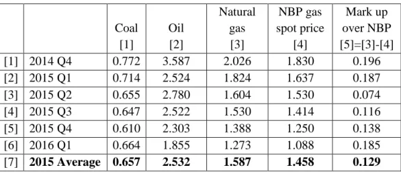
We use three set of fuel prices to see the impact of price granularity on our generation mix and interconnector flows from the modelling. The fuel prices are the averages of the prices delivered to major power stations as reported by DUKES statistics, which include transport and gas network charges, making these prices higher than the spot traded prices (see Table 2). As we treat all similar plants as identical, average rather than plant-specific fuel prices are appropriate. Table 1: Fuel prices used in the modelling (pence/kWhth)
Coal [1] Oil [2] Natural gas [3] NBP gas spot price [4] Mark up over NBP [5]=[3]-[4] [1] 2014 Q4 0.772 3.587 2.026 1.830 0.196 [2] 2015 Q1 0.714 2.524 1.824 1.637 0.187 [3] 2015 Q2 0.655 2.780 1.604 1.530 0.074 [4] 2015 Q3 0.647 2.522 1.530 1.414 0.116 [5] 2015 Q4 0.610 2.303 1.388 1.250 0.138 [6] 2016 Q1 0.664 1.855 1.273 1.088 0.185 [7] 2015 Average 0.657 2.532 1.587 1.458 0.129
Source: [1]-[3] DUKES (2018) Table 3.2.1; [4] Bloomberg terminal
First, we use 2015 average coal, oil and gas prices (columns 1-3, row 7, Table 2); secondly we use quarterly prices and finally we use quarterly coal and oil prices but daily NBP gas prices adjusted to account for costs of delivering from the NBP to the power stations (“mark up over NBP, column 5, Table 2). Then, we find a set of 𝑀𝑀𝑗𝑗 for coal, gas and interconnectors such that the difference between the model and real 2015 supply mix (annual resolution) is minimized.
Using either annual or quarterly fuel prices we were unable to obtain satisfactory results for the supply mix of 2015 – we could not find the multiplicative calibration parameter Mj that
would get us close to the observed supply mix of 2015. However, using daily gas and
interconnector prices with quarterly coal prices, Table 3 shows that there exists a set of Mj that
minimises the differences between annual supply in 2015 and the model results. The result delivers the annual supply mix extremely close to the actual 2015 mix.
19
Table 2: Calibration results for the year 2015 using daily gas prices and quarterly coal prices
Annual supply, TWh Supply mix
calibration parameter, 𝐌𝐌𝐣𝐣 2015 [1] Simulation [2] Delta [3]=[2]-[1] Interconnectors Britned (GB-NL) 8.00 7.93 -0.07 0.750 EWIC (GB-IE) -1.07 -1.10 -0.03 1.090 IFA (GB-FR) 13.85 13.92 0.07 0.800 Moyle (GB-NI) -0.19 -0.27 -0.08 1.090 Fossil fuel generation Coal 74.49 74.55 0.06 1.014 Gas 84.39 84.52 0.13 1.044 Hydro pumped storage Discharge 2.67 1.75 -0.92 n.a. Charge -3.57 -2.57 0.99 n.a.
The differences between the modelling results and the observed data is within 3% except for interconnector flows through Moyle and pumped storage stations. The absolute difference for flows over Moyle is relatively small but large in relative terms (42% over actual flows). We could further calibrate the flows for EWIC and Moyle by applying different calibration
parameters but deemed the results in Table 3 very satisfactory for our purposes. In 2015 neither EWIC nor Moyle were coupled to GB (IFA and BritNed were) and only managed to flow electricity in the right direction less than 60% of the time (SEM, 2017).
Differences in hydro PS reflect the fact that in the model the PS results are driven only by price arbitrage opportunities whereas in reality PS stations fulfil a number of balancing and ancillary services that are not captured in the current model. Further, Cruachan PS station has access to a catchment area and so enjoys natural inflows that might offer “free” storage. It is reported that 10% of annual electricity output from the Cruachan PS station is produced using rain and to that extent operates as a conventional run-of-river hydropower station (Scottish Power, 2011).
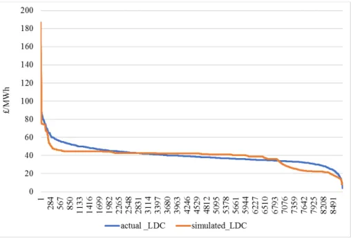
Finally, we compared the calibrated system marginal prices (SMP) with the 2015 GB day-ahead prices and found that, on average, our SMPs are 7.6% higher than the 2015 actual day-ahead prices. This is a result of ‘marking up’ fuel (gas by 4.4% and coal by 1.4%) and interconnector prices to achieve the 2015 supply mix (see Table 3). Therefore, we adjust the entire supply curve down by 7.6% and re-run the model to achieve the best possible fit in terms of annual supply mix (Table 3) and SMPs (Figure 2).
Applying these multiplicative fuel mix calibration parameters addresses the systematic biases in the quality of input data, such as fuel prices which are very heterogenous (specific to each plant and location), as well as systematic biases inherent to the modelling approach, such as determinism and perfect foresight. Using these multiplicative correction biases parameters for sensitivity and further scenario-based analysis appears defensible and more plausible than application of specific hourly mark-up parameter which is calibrated to historical data to get a very close match between model output and real data. In this regard, using this multiplicative
20
correction biases parameter for sensitivity and further scenario-based analysis is more plausible than, for example, hourly mark-up parameters calibrated to historical data.
Figure 2: GB load duration curves (LDC) – 2015 vs simulated results
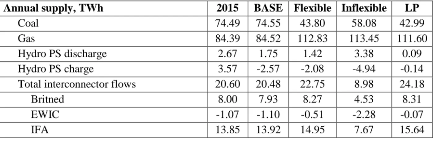
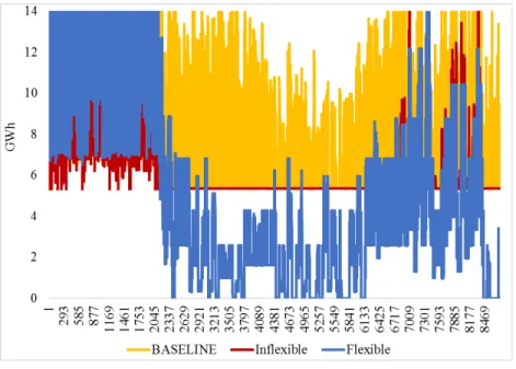
4.4. Sensitivity analysis
This section reports the sensitivity to structural features of the model. We take the calibrated baseline from §4.3 as the reference point and change the model structure along three key dimensions:
1. The length of the rolling modelling horizon, 2. The size of operating reserve requirements,
3. Binary and commitment decisions, plant flexibility parameters and simple economic dispatch solution without binary decisions.
4.4.1. Impact of modelling horizon length on results and solution time
The baseline sets the rolling horizon at 100 hours, that is, K=100. The cut-off time is 30% of this, i.e., 30 hours (see §3.3.1). One very important implication is that due to hydro PS
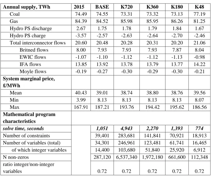
constraints (eq. 19 and 20) the longer is K the less the problem is ‘compact’ – the size of the model due to the summing over ‘t’ becomes huge. Table 4 shows this has a dramatic impact on the solution time without any meaningful improvement in the ‘quality’ of the results.
One can see that increasing the number of hours from 100 hours (baseline) to 720 hours (K720) increases the total solution time by a factor of five. However, the impact on the results is only a slight improvement in PS dispatch (i.e., an increase in PS utilization). This confirms our initial expectation that the number of hours in each horizon will most likely influence dispatch of units with intertemporal constraints such as eq. (19-20) for PS and conventional generation constraints related to minimum up and down time (eq. 11-16). It is interesting that the higher PS utilization is associated with higher outputs from gas plants, probably because gas prices varies
21
daily and hence PS can realize daily arbitrage opportunities more efficiently compared to coal quarterly prices.
There is some non-linearity in the relationship between the number of hours and PS utilization – K180 seems to produce the highest PS utilization while in K48 we see the lowest PS utilization. Again, this might be due to fuel price dynamics (gas prices in particular) in that a moving 180-hour optimization window might capture most of gas price volatility and hence higher PS utilization rather than a moving 720-hour window.
Table 3: Impact of modelling horizon length on results
Annual supply, TWh 2015 BASE K720 K360 K180 K48
Coal 74.49 74.55 73.31 73.32 73.13 77.19
Gas 84.39 84.52 85.98 85.95 86.26 81.25
Hydro PS discharge 2.67 1.75 1.78 1.79 1.84 1.67
Hydro PS charge -3.57 -2.57 -2.63 -2.64 -2.70 -2.46
Total interconnector flows 20.60 20.48 20.28 20.31 20.20 21.06
Britned flows 8.00 7.93 7.93 7.93 7.87 8.04
EWIC flows -1.07 -1.10 -1.12 -1.12 -1.13 -0.98
IFA flows 13.85 13.92 13.78 13.79 13.77 14.22
Moyle flows -0.19 -0.27 -0.30 -0.29 -0.30 -0.21
System marginal price, £/MWh Mean 40.43 39.01 38.74 38.80 38.76 39.56 Min 3.99 8.13 8.13 8.13 8.13 8.07 Max 167.91 187.21 193.76 194.42 195.62 186.56 Mathematical program characteristics
solve time, seconds 1,051 4,943 2,270 1,393 774
Number of constraints 39,401 283,681 141,841 70,921 18,913 Number of variables (total) 34,301 246,961 123,481 61,741 16,465 of which integer variables 14,400 103,680 51,840 25,920 6,912
N non-zeros 287,120 6,537,340 1,972,180 661,600 112,348
ratio integer/non-integer
variables 0.72 0.72 0.72 0.72 0.72
Note: solve time is reported for the entire modelling horizon of 14 months or 10248 hours.
All in all, one can see that a rather drastic change in the length of one modelling horizon from 48 hours to 720 hours produces results which are very similar. At least for this unit
commitment model of the GB electricity market the model time horizon should be 48-180 hours to reduce the solution time. As already noted, uncertainty about future demand, renewables
22
output and plant availability limit the time horizon over which operational systems optimize so optimizing beyond a couple of days may not make much sense.
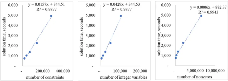
In general, the solution time increases linearly with the size of the optimization problem (Figure 3). However, the number of non-zeros (data that the model needs to process) slightly better explains the solution time than the number of constraints and variables. This highlights the importance of model’s compactness and the influence of this has on the solution time. For example, comparing model characteristics for the baseline and K720 shows that while the number of constraints and variables increases by a factor of 7.2, the number non-zeros increases by a factor of 22.8; and this increases the solution time by a factor of 4.7.
Figure 3: Solution time and the size of the unit commitment problem
The length of time horizon should be guided by the minimum up/down times as well as the total storage volume, as these parameters influence the optimality of each modelling horizon. For example, if coal stations have a minimum up (and down) time of 24 hours then it would be desirable to model at least 25 hours in one modelling horizon to ensure the model can decide on their commitment status. Similarly, if all PS stations can store up to 24 hours’ worth of energy then the modelling horizon should be at least twice 24 hours to account for one cycle of charge and discharge. This will ensure that we are not constraining the model and the search space when it comes to PS dispatch decisions.
The baseline and all the sensitivities were modelled on a 64-bit Windows 7 PC with 32 GB of RAM and 2 multi-core Intel Xeon CPU E5-2650 2.6 GHz processors (16 cores in total).8 The baseline has also been modelled on two other machines with different specifications to see how sensitive the solution time is to the spec of the PC:
23
1. 64-bit Windows 10 PC with 8 GB of RAM and one multi-core (4 cores in total) i5-4590 with 3.3 GHz processor;9
2. 64-bit Windows 10 Laptop with 16 GB of RAM and one multi-core (4 cores in total) i7-4702HQ with 2.20 GHz processor.10
We use AIMMS11 as the modelling environment and CPLEX solver version 12.7.1 with the MIP absolute optimality tolerance of 1e-6 and the relative optimality tolerance of 0.01. Rather surprisingly the solution time for the baseline on the i5-4590 machine was 593 seconds, almost twice as fast as the 2 multi-core processors machine. On a laptop, the solution time as significantly slower – 10,665 seconds. Clearly CPU clock speed significantly influences the solution time rather than the number of cores. This is principally because our model calibrated to the 2015 GB electricity market has a relatively small branch and bound tree and hence the number of cores does not matter too much.
4.4.2. Operating reserve and fast-ramping generation units
Dimensioning (sizing) operating reserve requirements is important in that it could greatly influence the dispatch order. For example, spin-up reserve requirement (eq. 3) will make sure that a certain amount of reserve capacity will be taken ‘off’ the dispatch order (supply curve). Traditionally, the spin-up reserve is equal to the capacity of the largest generation (or
interconnector) plus a percentage of demand to reflect possible errors in demand forecasting. But with the rapid uptake of VRE, the spin-up requirement also needs to consider forecast errors of the VRE resources (wind and solar). This means that operating reserves will become increasingly volatile. The volatility will be dependent on VRE capacity but also how much assurance a
system operator wants to have to hedge against forecasts errors. For example, the assurance will involve a decision whether to hedge against 99% of possible swings in demand and VRE
generation forecast errors (three standard deviations of forecast errors) or less (more) (see Appendix 1, A.3 for further discussions on this point). This section examines the impact of (i) sizing of the operating reserve, and (ii) types of units who can fulfil reserve requirements on modelling results.
In the baseline we define spinning up requirement as the sum of the capacity of the largest generator plus three standard deviations (SD, σ) of demand and wind forecast errors (see eq. A.6 in Appendix 1). Three SDs will cover 99% of the distribution of errors while four SDs will cover 99.99% while two SDs will cover 95%. Taking a zero SD means not considering errors in demand and VRE resource forecasts. The operating reserve is then static over the entire modelling horizon and equal to the capacity of the largest generating unit connected to the system. We also model a case without operating reserve (“no reserve” case) equations (3 and 4).
In eq. (3) both synchronized and non-synchronized units can bid into the spinning up reserve market. Non-synchronized units are fast ramping generators that can spin up very quickly
9 3.3 GHz base frequency and 3.7 GHz max turbo frequency 10 2.2 GHz base frequency and 3.2 GHz max turbo frequency 11 https://aimms.com/
24
(usually within an hour to reach full capacity). We allow both hydro PS and gas-fired generation to bid as synchronized units. In a sensitivity analysis we allow only hydro PS to bid as non-synchronized units, thus excluding all fast-ramping gas units from this market. The rationale here is to see whether this will impact hydro PS utilization.
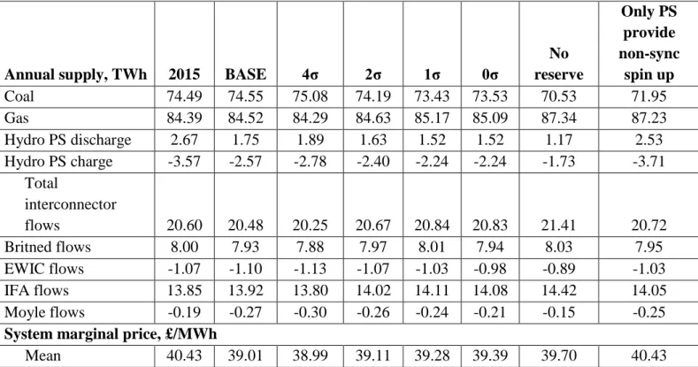
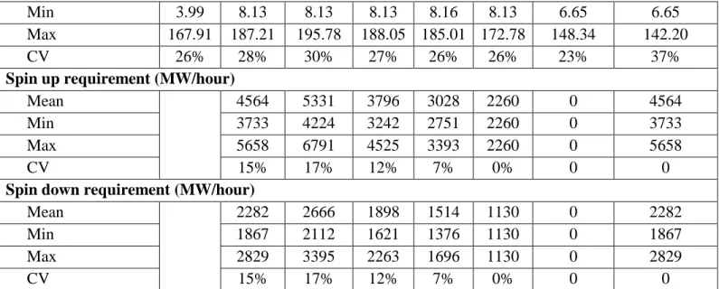
Table 5 reports our modelling results for different input assumptions around operating reserves. First, as we increase the ‘coverage’ of demand and VRE forecast errors in sizing of the operating reserve (from 0σ to 4σ), the volatility (measured as the coefficient of variation, CV) of hourly reserve requirements increases. Greater volatility implies a higher use of PS. With higher wind and solar penetration, the requirement for electric energy storage will likely increase, but more as a balancing and ancillary service provider rather than as purely price arbitrage. This can be seen by comparing the PS utilization in the “no reserve” case with the baseline Furthermore, the importance of PS in providing ancillary services (in our case non-synchronous spin-up capability) can be seen in the case when we restrict PS to provide spin-up capability as non-synchronous units only – in this case, the PS utilization is very close to the actual 2015 utilization level.
Second, higher volatility of reserve requirements means higher SMP volatility (compare baseline with 4SD and other cases in Table 5). It is also interesting that if PS is restricted to provide spin-up capability as the only non-synchronous units, the SMP volatility is the highest amongst all cases considered as it puts substantial pressure on synchronized units (coal and gas units who are already committed in the energy only market) to fulfil reserve requirements. Table 4: Impact of operating reserve requirements on modelling results
Annual supply, TWh 2015 BASE 4σ 2σ 1σ 0σ
No reserve Only PS provide non-sync spin up Coal 74.49 74.55 75.08 74.19 73.43 73.53 70.53 71.95 Gas 84.39 84.52 84.29 84.63 85.17 85.09 87.34 87.23 Hydro PS discharge 2.67 1.75 1.89 1.63 1.52 1.52 1.17 2.53 Hydro PS charge -3.57 -2.57 -2.78 -2.40 -2.24 -2.24 -1.73 -3.71 Total interconnector flows 20.60 20.48 20.25 20.67 20.84 20.83 21.41 20.72 Britned flows 8.00 7.93 7.88 7.97 8.01 7.94 8.03 7.95 EWIC flows -1.07 -1.10 -1.13 -1.07 -1.03 -0.98 -0.89 -1.03 IFA flows 13.85 13.92 13.80 14.02 14.11 14.08 14.42 14.05 Moyle flows -0.19 -0.27 -0.30 -0.26 -0.24 -0.21 -0.15 -0.25 System marginal price, £/MWh
25
Min 3.99 8.13 8.13 8.13 8.16 8.13 6.65 6.65
Max 167.91 187.21 195.78 188.05 185.01 172.78 148.34 142.20
CV 26% 28% 30% 27% 26% 26% 23% 37%
Spin up requirement (MW/hour)
Mean 4564 5331 3796 3028 2260 0 4564
Min 3733 4224 3242 2751 2260 0 3733
Max 5658 6791 4525 3393 2260 0 5658
CV 15% 17% 12% 7% 0% 0 0
Spin down requirement (MW/hour)
Mean 2282 2666 1898 1514 1130 0 2282
Min 1867 2112 1621 1376 1130 0 1867
Max 2829 3395 2263 1696 1130 0 2829
CV 15% 17% 12% 7% 0% 0 0
Note: CV – coefficient variation is determined as a ratio of standard deviation to the mean; 4σ means four standard
deviations (SD) of demand and wind forecast errors; 3σ – three SD and so on.
Third, in all our cases, non-synchronized gas-fired capacity will cover 99% of all spin-up reserve requirements (Table 6). It is only when we exclude non-synchronized gas-fired capacity from providing spin-up reserves is the spin up reserve market roughly equally divided between online coal and gas units as well as PS units.
All in all, defining operating reserve requirements is important as it will influence dispatch order and SMP. That said, our sensitivity analysis shows that the variations in annual output of gas and coal is of order of 4% and 7% respectively and 80% for PS. Clearly the impact on the PS utilization is the greatest.
Table 5: Provision of reserves by technology type, MW/hour (as % of hourly average reserve requirement) BASE 4σ 2σ 1σ 0σ Only PS provide non-sync spin up S pi n up res er v e synchronised coal 1 (0.0%) 1 (0.0%) 0 (0.0%) 0 (0.0%) 0 (0.0%) 2,139 (46.9%) synchronised gas 5 (0.1%) 14 (0.3%) 3 (0.1%) 0 (0.0%) 0 (0.0%) 2,414 (52.9%) Non-synchronised gas 4,557 (99.9%) 5,313 (99.7%) 3,793 (99.9%) 3,028 (100.0%) 2,260 (100.0%) 0 (0.0%) Non-synchronised PS 1 (0.0%) 2 (0.0%) 0 (0.0%) 0 (0.0%) 0 (0.0%) 8 (0.2%) S pi n dow n synchronised coal 843 (35.7%) 1,015 (37.1%) 664 (33.4%) 448 (27.9%) 243 (19.8%) 738 (31.4%)