Designing and Optimizing Representations for Non-Binary Constraints

(1)

DESIGNING AND OPTIMIZING

REPRESENTATIONS FOR NON-BINARY

CONSTRAINTS

WEI XIA

NATIONAL UNIVERSITY OF SINGAPORE

2014

(2)

DESIGNING AND OPTIMIZING

REPRESENTATIONS FOR NON-BINARY

CONSTRAINTS

WEI XIA

B.Eng., Northeastern University (China), 2009

A THESIS SUBMITTED FOR THE DEGREE OF

DOCTOR OF PHILOSOPHY

DEPARTMENT OF COMPUTER SCIENCE

NATIONAL UNIVERSITY OF SINGAPORE

(3)

Declaration

I hereby declare that this thesis is my original work and it has been

written by me in its entirety.

I have duly acknowledged all the sources of information which have

been used in the thesis.

This thesis has also not been submitted for any degree in any

univer-sity previously.

Wei Xia

July 16, 2014

(4)

Acknowledgment

I would like to thank my supervisor Dr. Roland Yap for guiding me to research and supporting me during these years. His extensive knowledge, broad research interest, and hard work were always encouraging me. He gave me many interesting ideas and constructive suggestions to develop and improve my research studies and skills. I feel lucky for the opportunity of being his postgraduate student.

I would like to thank Chavalit Likitvivatanavong for the valuable discussion and comments on this thesis.

I would like to thank my co-authors of the research papers, Kenil Cheng and Chavalit Likitvivatanavong. It has been a pleasure working with them.

I want to thank Behnaz Bassanshahi for proofreading the thesis. Finally, my thanks and love go to my parents and sister.

(5)

Summary

Global constraint plays a central role in constraint programming due to its strong modelling and ecient propagation. Table constraint is a general constraint as it can dene an arbitrary constraint extensionally, either as a set of solutions or a set of non-solutions, thus is able to represent any nite domain constraint. Table constraint can also be converted to and solved on other representations, such as multi-valued decision diagram (MDD), automaton and grammar.

In this thesis, we focus on the design, optimization and analysis of propagation algorithms for non-binary constraints with dierent representations. Some of these constraints, e.g. regular and grammar constraints, can also be thought as table constraints. We rst propose a generalized arc consistency (GAC) algorithm for the regularconstraint dened on non-deterministic nite automaton (NFA), called nfac. Thenfaccan also propagate the constraint represented by deterministic nite automaton(DFA) or MDD. We investigate the eect of dierent representations focusing on the space-time tradeos. Our experimental results show that nfac is faster when the NFA is much smaller than its equivalent DFA or MDD. We also extend nfac to grammarc for grammar constraint dened on context-free grammar (CFG) in Greibach normal form (GNF). Again we show thatgrammarc is faster on more compact grammars.

Second, we revise the state-of-the-art GAC algorithms, STR, for table con-straints, so that they can work on compressed representations. To be more spe-cic, the tables are compressed into the Cartesian product, which we call c-tuples. We extend the STR2 and STR3 algorithms to work with c-tuple. Our experiments show that compression can be signicant, the more the tables are compressible, the faster are the c-tuple algorithms.

(10)

stronger than GAC and have the potential of stronger search space reduction. However, higher-order consistencies are usually much more costly than GAC, and thus not many practical propagation algorithms have been designed or imple-mented. FPWC is a promising higher order consistency. Recently the eSTR algorithm adapts the STR2 GAC algorithm to enforce FPWC but it needs com-plex data structures which can impose signicant overheads. The k-interleaved

encoding is proposed to transform CSPs with dual variables and join tables, so that k-wise consistency (stronger than GAC) can be achieved though GAC.

How-ever the join tables in k-interleaved encoding may be large and thus slow down

the propagation algorithms. To contrast, we propose a dierent encoding to trans-form one CSP into another "equivalent" one, so that FPWC can be enforced on the original CSP through GAC on the transformed one. The key idea is to fac-tor out the commonly shared variables from constraints' scopes, form new com-pound variables, and re-attach them back to the constraints where they come from. These compound variables can be treated as a dierent representation designed for FPWC. Experiments show that our encoding with more compact representations can outperform the eSTR algorithm and the k-interleaved encoding. We again

demonstrate that both time and space eciency can be gained from a smaller representation.

(11)

List of Tables

3.1 Benchmarks for nfac. . . 30

3.2 Average construction time and solving time of nfac . . . 31

4.1 Runtime for the shift scheduling problem . . . 49

4.2 The grammar size of the forklift scheduling problem . . . 50

5.1 Statistics of the benchmarks . . . 73

5.2 Average runtime of the random benchmarks . . . 73

5.3 Comparison of the revised STR . . . 77

6.1 Mean results for FE . . . 98

(12)

(13)

List of Figures

2.1 An example of constraint graph . . . 6

2.2 Examples of local consistencies . . . 11

2.3 An example for solving a CSP . . . 12

2.4 Examples of dierent constraints . . . 18

3.1 Examples of NFA, DFA, and MDD representations . . . 20

3.2 Illustration of regularc . . . 23

3.3 NFA to MDD construction . . . 25

3.4 The nfac algorithm . . . 28

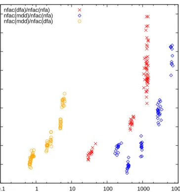
3.5 NFA versus DFA or MDD . . . 33

3.6 NFA versus regular. . . 33

3.7 The signicance of construction time . . . 34

4.1 An example of table V for CYK-prop . . . 39

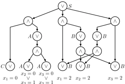
4.2 An example of AND/OR graph . . . 41

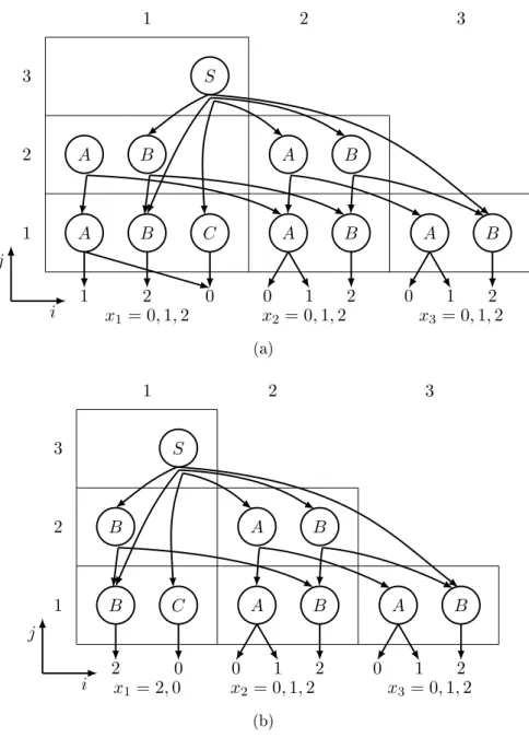
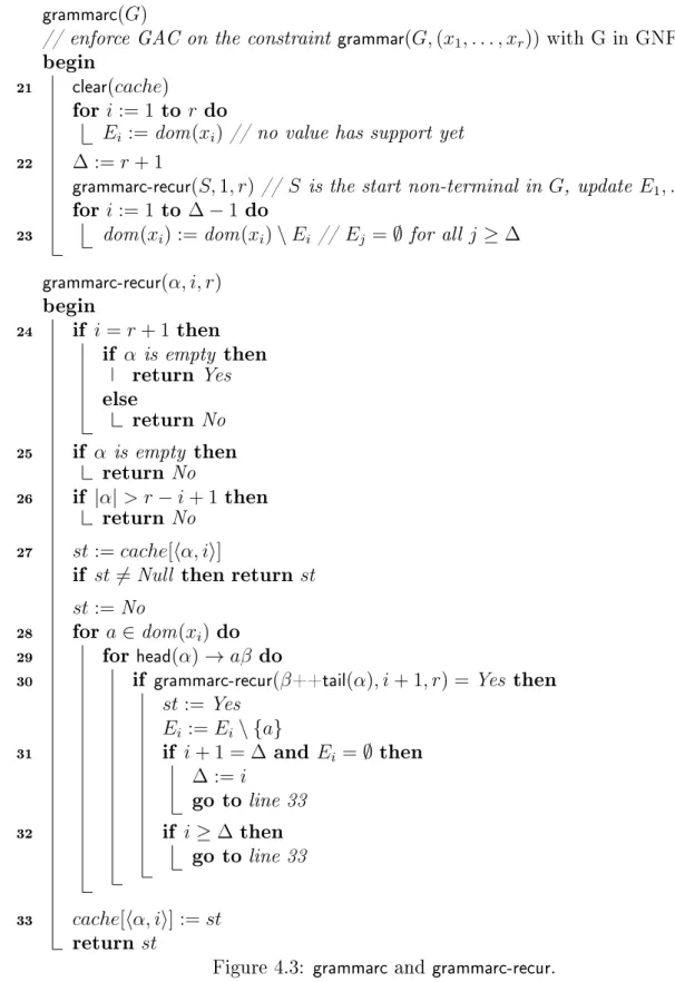
4.3 grammarc algorithm . . . 45

4.4 The pseudocode for the length optimization in grammarc . . . 46

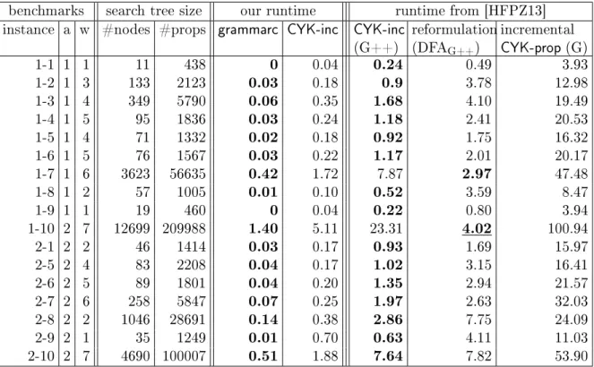
4.5 Runtime of grammarc and CYK-inc . . . 51

4.6 Runtime of grammarc on small and large GNF . . . 51

4.7 Comparison between grammarc/mddc and CYK-inc. . . 53

5.1 The STR1 algorithm . . . 57

5.2 The validity test of tuple . . . 58

5.3 Remove invalid tuple . . . 58

5.4 Restore invalid tuple . . . 58

5.5 Illustration of STR1 . . . 60

5.6 The table representation of STR3 . . . 61

5.7 The motif table of STRm-C . . . 63

5.8 The sliced table of STRsl-C . . . 65

5.9 Examples of short support . . . 66

(14)

5.11 The STR2-C algorithm . . . 68

5.12 The validity test of c-tuple . . . 69

5.13 The table representation of STR3 . . . 71

5.14 The STR3-C algorithm . . . 72

5.15 Runtime of STRx and STRx-C . . . 74

5.16 Runtime ratio versus compression ratio . . . 75

5.17 Runtime ratio versus average reduced table size . . . 75

6.1 Data structures of eSTR . . . 82

6.2 An example of k-interleaved encoding . . . 84

6.3 An example of factor encoding . . . 89

6.4 Representations of FE, kIL, and eSTR . . . 91

6.5 Examples of FE and FRJ . . . 94

A.1 STR2 algorithm. . . 119

A.2 The pseudocode of isValid(), removeTuple(), and restoreTuple() . . 120

A.3 STR3 algorithm. . . 121

(15)

Chapter 1 Introduction

Constraint Programming (CP) is a successful and useful approach to solve large combinatorial problems such as timetabling, scheduling, and resource allocation. These problems also appear in many industrial applications. Thus, constraint programming attracts both theoretical and commercial interest. A number of companies and researchers have put great eorts to develop the technologies in CP during the last thirty years.

Constraint programming provides a natural and ecient way to model and solve problems. A problem is rst modelled as a constraint satisfaction problem (CSP) with constraints stating its properties, and then solved by constraint solvers. Freuder states that as the following [Fre97]:

"Constraint programming represents one of the closest approaches computer science has yet made to the Holy Grail of programming: the user states the

problem, the computer solves it."

We contrast with integer programming, also a form of constraints, although integer programming is NP-complete, having only linear integer constraints is restrictive making problem modelling dicult. Rather in constraint programming, it is usual to have a whole range of constraints within the solver.

In practice, a problem can usually be dened with the developed constraints in a solver. Certainly, customized propagators for special constraints may also be developed. Since CSPs are NP-complete, search strategies and heuristics are used. Typically, constraint propagations to lter the inconsistent parts of CSPs work hand in hand with search strategies to reduce search space.

Many constraint programming solvers have been developed. Some represen-tative ones are Gecode [Gec], Abscon [Abs] and ILOG [Ilo]. Gecode is a widely used open source constraint solving toolkit. We evaluate our work with Gecode in Chapter 3 and Chapter 4. Abscon is another freely available CSP solver, which

(16)

has been used extensively in many papers, e.g. [Lec11], [LPRT12], [LPRT13], etc. We also use Abscon to conduct our experiments in Chapter 5 and Chapter 6.

This thesis addresses one of the challenges of constraint programming: design-ing expressive constraints together with ecient propagation algorithms. In par-ticular, we investigate the propagation algorithms on non-binary table constraints which are the most general form of nite domain constraints, and the eect of compact representations which can still represent tables. A number of ecient generalized arc consistency (GAC) propagation algorithms have been developed, with mddc [CY10] and various STR [Ull07, Lec11, LLY12] being the state-of-the-art ones for table constraints. Although mddc and STR vary in performance on dierent benchmarks, they are both based on compact representations: mddc uses multi-valued decision diagram (MDD) and STR uses table reduction. This sug-gests that a well designed propagation algorithm on a compact representation may save both time and space in practice.

In this thesis, we study the eect of the choices of representations on propaga-tion algorithms and consistency levels of CSPs. The variants of the two state-of-the-art GAC algorithms mddc and STR are rstly investigated with the principle that one table can have dierent representations.

The mddc algorithm enforces GAC on an MDD which provides an alternative representation of a table. Theregular constraint is originally dened on determin-istic nite automata (DFA), but can also be on non-determindetermin-istic nite automata (NFA) or MDD, or even be converted into a plain table. It is well known that an NFA can be exponentially smaller than its equivalent DFA. The table or MDD corresponding to the NFA of a regular constraint can also be large. Therefore, we investigate the eect of these dierent grammar representations on the eciency of GAC algorithms. We develop a new GAC algorithmnfac for theregularconstraints which can be represented by NFAs, DFAs, or even MDDs. We then extendnfacto grammarc on grammar constraints and show that grammarc is comparable with the state-of-the-art GAC algorithms for grammar constraints.

STR algorithms compress tables dynamically during search, i.e. removing the invalid tuples as search goes deeper and restoring them when backtrack happens. The key feature of STR is that table is shrunk dynamically in search. We propose to compress the tables with the Cartesian product representations statically before search. This thus requires a new STR algorithm which can work on the compressed representations. The Cartesian product representation was used in the context of symmetry breaking [FM01] and nogood learning [KB05] respectively. It was also applied to the GAC algorithm GAC-allowed [BR97] for table constraints and shown to speed up GAC-allowed [KW07]. However, unlike GAC-allowed where

(17)

compression is likely to be benecial on static tables, STR may have interplay between the static and dynamic compression, changing the benets respectively. GAC-allowed is no longer state-of-the-art. Our experimental results show that our revised STR algorithms are faster than the original algorithms when there is a reasonable amount of static compression. Recently, some other compressed table representations were introduced to STR [JN13, GHLR13, GHLR14]. Compared with these STR variants, ours appear to gain better compression and speedup on the common benchmarks used in all these papers.

The propagation algorithms of GAC are the most well researched for non-binary constraints and have been shown useful in practice. Many solvers have been developed with variants of ecient GAC algorithms. As an alternative to GAC or arc consistency (AC), higher-order consistencies have been proposed to get more pruning and propagations than GAC. However, higher-order con-sistencies are costly and require the development of new complex propagation algorithms. Although some higher-order consistency algorithms have been pro-posed [BSW08, KWR+_{10], they are not usually presented or implemented in the}

CP solvers in common use. A general perception is that higher-order consistencies may not be practical, while this may not be entirely accurate. In practice, GAC is the propagation that one can expect in all mature CP solvers. Higher-order consistencies on the other hand are quite rare or may not be supported. Hence, we propose a transformation that encodes a non-binary CSPP into another P0 _so

that GAC on P0 _{guarantees full pairwise consistency (FPWC), a practical}

higher-order consistency, on P. We compare our approach with the k-interleaved

encod-ing from [MDL14] as well as the state-of-the-art FPWC algorithm eSTR [LPS13]. Our encoding implies two benets. First, higher-order consistency can be achieved without any change to the existing CP solvers with GAC propagators. Second, compared with k-interleaved encoding and the specialised FPWC algorithm, our

encoding uses more compact representations and is more ecient than the other two in our experiments.

In addition, we construct various new benchmarks for the experiments in this thesis in order to test and understand how dierent propagation algorithms behave. Good benchmarks are essential for further improvements of the algo-rithms. Some of the benchmarks are hard CSPs constructed based on Model RB/RD [XBHL05], so that the algorithms can be exercised. In particular, the feature of our benchmarks is that they either have a lot variance in the size of representations, or can be transformed into other equivalent representations with dierent sizes. For example, in Chapter 3, we generate several groups of NFAs which then can be converted into DFAs and MDDs with dierent sizes. With these

(18)

CSPs, we can evaluate the space-time tradeos of the GAC algorithms for the con-straints represented in automatons and MDDs. In Chapter 5, we construct CSPs by enlarging the existing table constraints, so that the amount of compression varies and we can investigate the eect of table compression on the algorithms. Outline of the thesis.

The thesis is organized as follows:

In Chapter 2, we introduce the background for constraint satisfaction prob-lems (CSP), the CSP solving process, various local consistencies, and some representative global constraints that are related to the rest of the thesis. In Chapter 3, we investigate the eect of constraint representations on the

space-time tradeos for the regularconstraints.

In Chapter 4, we give a GAC algorithm forgrammarconstraints and compare it with existing algorithms.

In Chapter 5, we develop two new STR algorithms which take the benets of the compressed table representations.

In Chapter 6, we propose to transform a CSP into another one, so that higher-order consistency can be achieved through GAC propagation.

In Chapter 7, we conclude the thesis and discuss the future work. List of publications.

[1] Kenil C. K. Cheng, Wei Xia, and Roland H. C. Yap, "A Space-Time Tradeos for the Regular Constraint", in Proceedings of the 18th International Conference on Principles and Practice of Constraint Programming (CP'12), pp.223-237, Québec City, Canada, 2012.

[2] Wei Xia and Roland H. C. Yap, "Optimizing STR Algorithms with Tuples Compression", in Proceedings of the 19th International Conference on Principles and Practice of Constraint Programming (CP'13), pp.724-732, Uppsala, Sweden, 2013.

[3] Chavalit Likitvivatanavong, Wei Xia, and Roland H. C. Yap, "Higher-Order Consistencies Through GAC on Factor Variables", to appear in Proceedings of the 20th International Conference on Principles and Practice of Constraint Program-ming (CP'14), Lyon, France, 2014.

(19)

Chapter 2 Background

In this chapter we introduce the denitions of constraint satisfaction problems, the terminologies of solving CSPs, an overview of global constraints, and other backgrounds.

2.1 Basic Denitions

Constraint satisfaction problem. A constraint satisfaction problem (CSP) or constraint network (CN) is a triple P = (X,D,C), where X = {x1, . . . , xn} is a

set of variables, D={D(x1), . . . , D(xn)} is a set of nite domain of the variables

and C ={c1, c2, . . . , cm} is a set of constraints.

Variable and domain. A variable x can only take values from its domain D(x). W.l.o.g., we will use a nite set of non-negative integers as a variable's

domain. The domain of a variable can be represented as an enumerated set or an interval with smallest and greatest values. For example, the domain of x can be

an enumerated set D(x) = {1,3,5} or an interval D(x) = [1,1000]. The size of

the domain ofxis denoted by|D(x)|. A Boolean variablexhas a Boolean domain D(x) ={0,1}, whose size is two.

An assignment (x, a) denoting x = a maps a variable x to value a ∈ D(x).

For a set of assignments θ={(xi1, ai1), . . . ,(xij, aij)}, the projection of θ on a set

of variables S is θ[S] = {(x, a)|(x, a) ∈ θ, x ∈ S}, and the projection of θ on a

particular variable isθ[x] =a if (x, a)∈θ.

Constraint. A constraint c is a relation dened on a set of distinct variables

(xi1, . . . , xir). The scope of c, denoted by scp(c), is (xi1, . . . , xir). The number

of variables in scp(c) is the arity of the constraint. The relation of c, denoted

by rel(c), is the set of value combinations of the variables in the scope of c that

(20)

The relation rel(c) can be extensionally represented by a table, which is a set of

r-ary tuples. We may use a tuple τ = (a1, . . . , an) to refer to a set of assignments

{(x1, a1), . . . ,(xn, an)} when the variables are clear, and τ[xi] = ai or τ[S] =

(ak1. . . , akn) (S is a set of variables and xkm ∈ S). A tuple τ = (a1, . . . , an)

is valid if ai ∈ D(xi) for ∀xi. Note that variables' domains can change, e.g.,

instantiated during search. A tuple τ is allowed by a constraint c, or satises c i τ[scp(c)] ∈ rel(c). A constraint can also be represented intentionally as

a formula. For example, let c(x, y) be a constraint requiring that the variables

x : D(x) = {0,1,2} and y : D(y) = {0,1,2} cannot take the same values at the

same time. The intentional representation of c(x, y) is x6=y and the extensional

representation with satisfying tuples is {(0,1),(0,2),(1,0),(1,2),(2,0),(2,1)}.

A constraint is unary if its arity is one1_{, or binary if its arity is two, or} non-binary otherwise. A CSP is non-binary if all of its constraints are unary or non-binary; otherwise it is non-binary. Two constraints ci and cj are equivalent, written as

ci ≡cj, if they express the same relations and have the same scopes.

Constraint (hyper) graph. A CSP is usually associated with a constraint (hyper) graph revealing the structure of the CSP. The vertices and the edges (or hy-peredges) correspond to the variables and constraints respectively. A constraint's corresponding edge (or hyperedge) linking dierent vertices indicates that the variables of the vertices belong to the scope of the constraint.

Solution. A solution of a CSP P = (X,D,C) is a set of assignments

{(x1, a1), . . . ,(xn, an)} such that all the constraints in C are satised.

Two CSPs are equivalent if they have the same set of solutions.

Example 2.1. Consider the CSP({x, y, z},{D(x) ={1,2}, D(y) = {1,2}, D(z) =

{2,3}},{x6=y, x6=z, y 6=z})whose constraint graph as shown in Figure 2.1. The

three binary constraints state that every pair of the variables must take dierent values. The set of assignmentsθ ={(x,1),(y,2),(z,3)}satisfy all the constraints.

Thus, θ is a solution of the CSP.

y z

x cx6=y ={12,21}

cy6=z={12,13,23}

cx6=z ={12,13,23}

Figure 2.1: An example of constraint graph.

(21)

2.2 Local Consistencies

Local consistency is the central idea in constraint programming. Informally, a certain local consistency denes a partially consistent status of a CSP, which can be achieved by removing certain inconsistent parts of the problem, so that the search space can be narrowed. The constraint propagation or ltering algo-rithms are developed to enforce dierent kinds of local consistencies of a CSP. We remark that local consistencies are separate from the propagation algorithms to enforce them, that each local consistency may have many dierent corre-sponding algorithms which undertake the propagation operations. For exam-ple, the propagation algorithms for AC include AC-3 [Mac77a], AC-4 [MH86], AC-2001 [BR01, ZY01, BRYZ05], etc. In this section, we introduce several rep-resentative local consistencies proposed for non-binary CSPs. The propagation algorithms of the local consistencies are introduced in the related chapters.

The local consistencies for non-binary CSPs can be divided into two classes depending on whether the consistencies alter the constraint graph or the relations of the constraints. The local consistencies which only lter the inconsistent values from the domains of variables and not alter the structure of the constraint graph or the relations of constraints are called the domain ltering consistencies [DB01]. The propagation algorithms for domain ltering consistencies are easier to imple-ment and easier to integrate with other propagation algorithms or various existing constraint solvers because they only update the domains of variables.

Generalized arc consistency. A value (x, a) is generalized arc consistent

(GAC) [Mac77b] i for all c∈ C where x ∈ scp(c), there exists at least one valid

tuple τ ∈ rel(c) such that τ[x] = a. This tuple τ is called a support for (x, a) in

c. A variable x ∈ X is GAC i every value a ∈ D(x) is GAC. A constraint c is

GAC i every variable x∈scp(c)is GAC. A CSP is GAC i every constraint inC

is GAC. GAC is used for non-binary CSP, while specically arc consistency (AC) is used for binary CSP.

GAC is the most well known and researched local consistency for non-binary CSPs. It is the local consistency available in most of current constraint solvers. Informally, GAC removes the domain values with no supports in a constraint. Thus, it is a domain ltering consistency. The propagation for GAC is based on reasoning with one constraint at a time. A number of dierent ltering algorithms have been developed to enforce GAC on table constraints.

Before we introduce more domain ltering consistencies, we dene how to com-pare the pruning power among dierent local consistencies following the denitions introduced by Debruyne and Bessiere [DB01]. A consistency φ is stronger than

(22)

another consistency ψ i for any problem P, φ holds on P implies that ψ also

holds on P. Also, φ is strictly stronger than another consistency ψ, denoted by φ →ψ, i φ is stronger than ψ and there exists at least one problem P0_, _ψ _holds

but φ does not, or P0 _is _ψ _{but not} _φ_. _φ _and _ψ _{are incomparable, denoted by}

φL

ψ, i φ is not stronger than ψ nor vice versa.

Below we introduce more domain ltering consistencies [BSW08] related to this thesis. As indicated by Bessiere et al. [BSW08], the following domain ltering consistencies are inspired by the corresponding local consistencies on binary con-straints. They are stronger domain ltering consistencies than GAC for non-binary constraints. The challenge is that stronger consistencies can lter more inconsis-tent parts of CSPs but require higher time complexity than GAC. Thus higher-order consistencies may not be benecial in practice sometimes. In Chapter 6.1 of this thesis, we propose to encode one CSP into another such that enforcing GAC on the latter guarantees a stronger consistency on the former.

Relational path inverse consistency [BSW08]. A value(x, a)is relational

path inverse consistent (rPIC) i∀ci ∈ C, wherex∈scp(ci), and∀cj ∈ C such that

scp(ci)∩scp(cj)6=∅, ∃τ ∈rel(ci)such that τ[x] =a,τ is valid, and∃τ0 ∈rel(cj)

such that τ0 is valid and τ[scp(ci)∩scp(cj)] = τ0[scp(ci)∩scp(cj)]. A variable

x ∈ X is rPIC i every value a ∈ D(xi) is rPIC. A CSP P is rPIC i every

variable x∈ P is rPIC.

From the above denition, rPIC does not require cj and cl to be dierent,

so that rPIC implies GAC. On top of GAC, rPIC considers pairs of constraints with sharing variables, and the values with supports in one constraint but cannot be extended to the second constraint are inconsistent. Thus, rPIC is stronger than GAC. Its corresponding consistency on binary CSPs is called path inverse consistency (PIC) [FE96].

Restricted pairwise consistency [BSW08]. A value (x, a) is restricted

pairwise consistent (RPWC) i a is GAC and ∀ci ∈ C, where x ∈ scp(ci), such

that there exists a unique valid tupleτ ∈rel(ci)withτ[x] =a, and∀cj ∈ C(ci 6=cj)

such that scp(ci)∩scp(cj)6=∅, ∃τ0 ∈rel(cj) such that τ0 is valid andτ[scp(ci)∩

scp(cj)] =τ0[scp(ci)∩scp(cj)]. A variablex∈ X is RPWC i every valuea∈D(x)

is RPWC. A CSP P is RPWC i every variablex∈ P is RPWC.

RPWC restricts the values to be GAC, but it is not much stronger. RPWC only treats the values with unique support in one constraint as inconsistency if such a support cannot be extended to a valid tuple in all the other constraints with sharing variables. RPWC's corresponding consistency on binary CSPs is restricted path consistency (RPC) [Ber95].

(23)

restricted pairwise consistent (MaxRPWC) i ∀ci ∈ C, where x ∈ scp(ci), ∃τ ∈

rel(ci) such that τ[x] = a, τ is valid, and for all cj ∈ C(ci 6= cj) such that

scp(ci)∩scp(cj)6=∅, ∃τ0 ∈rel(cj) such that τ0 is valid andτ[scp(ci)∩scp(cj)] =

τ0[scp(ci)∩scp(cj)]. In this case, τ0 is a PW-support of τ and τ is a

maxPRWC-support of (x, a). A variable x ∈ X is MaxRPWC i every value a ∈ D(x) is

MaxRPWC. A CSP P is MaxRPWC i every variable x∈ P is MaxRPWC.

MaxRPWC also implies GAC, but is stronger than the previous two consis-tencies, rPIC and RPWC. Relational path inverse consistency is limited to pair of constraints, thus one valid tuple of a constraint extendable to one intersecting constraint may not be extendable to another. But for MaxRPWC, once a sup-port τ is found for a value a in one constraint, τ will be checked against all the

other constraints with sharing variables. Only when PW-supports are found for all the sharing constraints,τ is treated as a MaxRPWC-support for valuea. Thus

MaxRPWC is stronger than rPIC. MaxRPWC is also stronger than RPWC, as RPWC only considers a special case of MaxRPWC. Similar to rPIC and RPWC, MaxRPWC also has its corresponding consistency max restricted path consistency (MaxRPC) [DB97] in binary CSP.

The second class of local consistencies alters the constraint graph or the rela-tions of constraints. These local consistencies include path consistency [Mon74], relational consistency [vBD95], singleton generalized arc consistency (SGAC) [DB01], pairwise consistency (PWC) [JJNV89], etc. Compared with the domain ltering consistencies, which are easier to be integrated with the existing CP solvers, it is more dicult to design and implement ecient propagation algorithms for these local consistencies in practice. Here we dene PWC andk-wise consistency, which

will be discussed more in Chapter 6.

Pairwise consistency [JJNV89]. A CSP P is pairwise consistent (PWC)

i for any constraint ci, ∀τ ∈ rel(ci), if τ is valid, ∀cj(ci 6= cj), ∃τ0 ∈ rel(cj) s.t.

τ[scp(ci)∩scp(cj)] =τ0[scp(ci)∩scp(cj)] and τ0 is valid.

Instead of ltering variables' domains, PWC removes the consistent tuples of a constraint c that cannot be consistently extended to the other constraints with

sharing variables. Because GAC is easier to implement and cheaper than PWC, PWC is enforced together with GAC, so that the values of variables' domains can be pruned.

Full pairwise consistency [JJNV89]. A CSP P is full pairwise consistent

(FPWC) i the CSP is both PWC and GAC (PWC+GAC). PWC is generalized to k-wise consistency [Gys86].

K-wise consistency [Gys86]. A CSPP isk-wise consistent (kWC) i given

(24)

j there exists a valid tuple τ0 over Sk

l=1scp(cil) such that τ

0_[_scp₍_c

ij)] = τ and τ0[scp(cil)] ∈ rel(cil) for all l ∈ {1, . . . , k}. When k equals to two, it reduces to

PWC. If P iskWC (k _>3) then P is (k-1)WC. Same as PWC,kWC can also be

enforced together with GAC.

GAC+kWC. A CSPP is GAC+kWC i P is both GAC and kWC.

The following theorem, based the theorem proposed by Bessiere et al. [BSW08], states the ltering power among the local consistencies introduced above.

Theorem 2.1. kWC+GAC (k >2)→ FPWC→ maxRPWC→rPIC→ RPWC

→ GAC

The following example shows the dierences among the above consistencies. Example 2.2. In Figure 2.2, the example compares dierent consistencies when considering the ltering of value(x1,0). The domains of the variables areD(x1) = D(x4) = D(x5) = {0}, D(x2) = D(x3) = {0,1}. Figure 2.2(a) illustrates GAC.

Figure 2.2(b) to Figure 2.2(e) are for the consistencies stronger than GAC. The sharing variables between dierent constraints are x2 and x3.

Figure 2.2(a) only gives one constraint as GAC works with one constraint at one time. It shows that (x1,0) of c1 is GAC as the value has supports

(0,0,0) and (0,1,1) in the constraint.

In Figure 2.2(b), when considering x1 for RPWC,(x1,0)has more than one

support, then no need to check whether the tuples in c1 are extendable to c2.

Thus, (x1,0) is RPWC, although no supports in c1 can be extended to c2.

In Figure 2.2(c), when considering x1 for rPIC, the tuple (0,0,0)is

extend-able to c2 and the tuple (0,1,1) is extendable to c3, so that (x1,0) is rPIC.

However, if MaxRPWC is applied, (x1,0) is not consistent, as neither of its

supports in c1 can be extended to c2 or c3 at the same time.

Figure 2.2(d) gives an example that (x1,0) is MaxRPWC, as its support (0,0,0) in c1 can be extended to both c2 and c3. The valid tuple (0,0,0) in c2 and the valid tuple (0,0,0) in c3 are the PW-supports of (0,0,0) in c1.

Thus, (0,0,0) in c1 is the MaxRPWC-support of (x1,0).

Lastly, Figure 2.2(e) shows an example for FPWC. The tuples marked with

× should be removed from the table, as they cannot be extended to satisfy

the other two constraints. This is the key dierence from the previous four domain ltering consistencies. In addition, for FPWC, (x1,0) is consistent

(25)

c1 x1 x2 x3 0 0 0 0 1 1 (a) GAC c1 x1 x2 x3 0 0 0 0 1 1 c2 x2 x3 x4 0 1 0 1 0 0 (b) RPWC c1 x1 x2 x3 0 0 0 0 1 1 c2 x2 x3 x4 0 0 0 0 1 0 c3 x2 x3 x5 1 1 0 0 1 0 (c) rPIC c1 x1 x2 x3 0 0 0 0 1 1 c2 x2 x3 x4 0 0 0 1 1 0 c3 x2 x3 x5 0 0 0 0 1 0 (d) maxRPWC c1 x1 x2 x3 0 0 0 0 1 1 × c2 x2 x3 x4 0 0 0 1 1 0× c3 x2 x3 x5 0 0 0 0 1 0 × (e) FPWC

Figure 2.2: Examples of dierent local consistencies.

2.3 Solving CSPs

Constraint Propagation. Constraint propagation is a process of repeatedly re-moving inconsistent domain values and/or inconsistent parts of constraints while maintaining an equivalent CSP [Apt03]. The ltering algorithm of a constraint is an algorithm determining the inconsistent parts with respect to the constraint. During constraint propagation, various ltering algorithms are scheduled (for ex-ecution) and executed until a x-point is reached, which indicates that a certain local consistency is achieved or empty domains are found.

A CSP is usually solved through the combination of search and constraint propagation. The search is divided into two kinds: systematic search and local search. Systematic search guarantees to get the solutions to a CSP or nd out that the CSP is unsatisable. In this thesis, we focus on systematic search. Local search is dierent from the systematic search and incomplete. It typically instantiates all the variables of a CSP and changes the values based on certain heuristics. Thus, local search may not nd out the solution even if the CSP has one.

(26)

is a complete CSP solving algorithm for binary CSPs. It applies systematic search and enforces arc consistency once a variable is instantiated during search and back-tracks when a failure occurs. We may use MGAC to emphasize the applications to non-binary CSPs and GAC ltering algorithms. M(G)AC is one of the most ecient algorithms to solve large and hard CSPs, due to its ecient core (G)AC algorithms.

We illustrate the behaviour of MAC on Example 2.1. The search tree in Fig-ure 2.3 shows the solving process for all solutions of the CSPs. The dashed line indicates the propagation at one search node. At the beginning, MAC calls AC algorithms repeatedly on each constraint until the CSP is AC at a x-point. In this example, the network is initially arc consistent so that the domains of the variables are not changed at the root node. Then assume that x is rst assigned

to1 and enforce AC, we get:

y= 2 from the inference on x6=y;

z = 3 from the inference on y6=z and x6=z.

As a result, the rst solution is found. Then to nd the next solution, the search backtracks to the root node to try value 2 of x, and gets:

y= 1 from the inference on x6=y;

z = 3 from the inference on x6=z and y 6=z.

At this point, the search space is fully explored with two solutions{(x,1),(y,2),(z,3)}

and {(x,2),(y,1),(z,3)} found. x={1,2},y={1,2},z={2,3} x={1,2},y={1,2},z={2,3} x={2},y={1,2},z={2,3} x={2},y={1},z={3} x={1},y ={1,2},z={2,3} x={1},y ={2},z={3}

Figure 2.3: An example for solving a CSP using MAC.

2.4 Global Constraints

One of the key advantages of constraint programming over the other program-ming techniques is the introduction of global constraints, which can simplify the modelling of problems. The constraint with the following properties is usually treated as a global constraint. First, the scope of the constraint can be dened on any number of variables. Second, the constraint has specic semantics or data structures and occurs commonly in many applications. Third, ecient ltering

(27)

algorithms can be designed based on the semantics or the structures of the con-straints.

One of the most useful global constraints is the alldierent(x1, . . . , xr)

con-straint [Lau78, Rég94], which requires all the variables of the concon-straint to take dierent values. With the alldierent constraint, some problems' modelling be-come simple. For example, the three constraints in Example 2.1 can be re-placed by one alldierent(x, y, z) constraint. Another example is the Sudoku

prob-lem [Wik13, DdlB14]. Assume that the Sudoku probprob-lem has a 9×9 grid, then

it can be modelled with 27 alldierent constraints of arity 9. Without alldierent constraints, the modelling will include 810 inequality (6=) constraints.

A number of other global constraints have been developed, such as the global-cardinality constraint [Rég96], the stretch constraint [Pes01], the regular con-straint [Pes04, CB04], etc. Some global concon-straints can be represented by or converted into others, so that an ecient ltering algorithm for one constraint may be used by other constraints. For instance, it is mentioned in [Pes04] that the stretch constraint [Pes01] can be encoded as an automaton and expressed by aregular constraint. In addition, a regularconstraint can be converted into a table constraint by listing all the strings of xed length in its regular language. Further-more, such a table constraint can be transformed into a constraint represented by a multi-valued decision diagram (MDD) [SKMB90], called MDD constraint, us-ing the algorithm introduced by Cheng and Yap [CY10]. Therefore, we see that there can be many possible representations for one constraint, which is a question investigated in this thesis.

In the rest of this section, we dene theregularconstraint, table constraint, and MDD constraint [CY08, CY10] in detail, as they are the core constraints of this thesis.

2.4.1 Formal Language Theory

In this subsection, we give some denitions from the formal language theory. The denitions in this subsection are based on [HU79] and [RS97].

Deterministic nite automaton. A deterministic nite automaton (DFA) is a nite state machine represented by a 5-tuple(Q,Σ, δ, q0, F)whereQis a nite

set of states,σ is a nite set of input symbols called the alphabet, δ is a transition

function Q×Σ → Q, q0 ∈ Q is a start state, and F ⊆ Q is a set of nal or

accepting states.

Non-deterministic nite automaton. A non-deterministic nite automa-ton (NFA) is also a nite state machine represented by a 5-tuple (Q,Σ, δ, q0, F)

(28)

with dierent transition function thatδ :Q×Σ→P(Q), whereP(Q)is the power

set of Q. Informally, the transition δ(q, a) of a DFA will sink to one state; while

the transition of an NFA will sink to a set of states.

Regular language. We rst generalize the notation of δ to δ∗ taking a

se-quence of values as parameters. Given a strings,δ∗(q, s) =δ∗(δ(q, head(s)), tail(s)),

where head(s) is the rst symbol of s and tail(s) is the sub-string of s following head(s). A string s is accepted by a DFA (NFA)A= (Q,Σ, δ, q0, F)if δ∗(q0, s)is

(contains) a nal state in F. The language of a DFA (NFA) is dened by L(A) ={s|s is accepted by A}

If a language L is L(A)for some DFA (NFA) A, thenL is a regular language.

Context-free grammar. A context-free grammar is a 4-tupleG= (V, T, P, S)

where V is a set of nonterminal symbols, T is a set of terminal symbols or called

the alphabet, P is the set of productions and S is the start symbol. A production

is a rule A → α where A is a nonterminal and α is a sequence or nonterminals

and terminals.

Give a grammar G, we denote the size of the grammar by |G|, that |G| =

P

p∈P|p|, where |p| is the number of terminals and non-terminals in productionp.

We use ⇒ to indicate one-step derivation of applying the productions to replace

the head by the body. Similar to the extension of δ toδ∗, we generalize ⇒ to ⇒∗

to denote zero or more steps of derivations. A string w of terminal symbols can

be generated by a CFG G= (V, T, P, S)i S ⇒∗ w.

Context-free language. The language of a CFG G= (V, T, P, S)is dened

by

L(G) = {w∈T∗|S ⇒∗ w with the productions ofG}

If a language L is L(G) for some CFG G, then L is a context-free language.

Before ending this subsection, we give two important and useful normal forms of CFG.

Chomsky normal form. A context-free grammar is in Chomsky normal form (CNF) if all of its production rules are of the forms:

A→BC

or

A→a

where A, B, and C are all non-terminals and a is a terminal. Every CFG can be

converted into an equivalent CNF. A transformation algorithm can be found in the book [HMU06]. CNF is useful in practice as it can provide ecient membership

(29)

tests of a string in a context-free language. Moreover, an ecient propagation algorithms for grammar constraints based on CNF is also proposed recently, which will be introduced later in Chapter 4.

Greibach normal form. A context-free grammar is in Greibach normal form (GNF) if all of its production rules are of the forms:

A→aα

where A is a non-terminal, a is a terminal, and α is a string of non-terminals. It

is shown by Greibach [Gre65] that every CFG can be converted into an equivalent GNF. GNF is useful in many theoretical proofs. For instance, it can be used to show that every context-free language can be accepted by a pushdown automaton (PDA).

2.4.2 Formal Language Constraints

In this subsection, we introduce two global constraints for automata and gram-mar respectively: the regular constraint [Pes04, CB04] and the grammar con-straint [QW06, Sel06]. In practice, these two concon-straints are quite useful, espe-cially in scheduling, rostering and sequencing problems, because they can express complicated patterns more simply.

Regular constraint [Pes04]. Let A= (Q,Σ, δ, q0, F)be a DFA and X be a

sequence of variables with nite domains. A regular(X, A) constraint states that

any sequence of values taken by the variables of X must belong to the regular

language recognized byA.

Example 2.3 and Figure 2.4 give four constraints with the same relations but dened on dierent representations. Among them, Figure 2.4(c) shows an example of a regular constraint on DFA. Althoughregularconstraint is originally dened on a DFA, it can also be on an NFA. To emphasize the actual representation, in the rest of this thesis, theregularconstraint dened on an NFA or a DFA will be named as an NFA constraint or a DFA constraint. The NFA constraint might be useful, as the NFA may have exponentially fewer states than an equivalent DFA, and this size dierence may further aect the eciency of the propagation algorithms when solving a problem.

Grammar constraint [QW06]. Let G= (V, T, P, S) be a CFG and X be a

sequence of variables with nite domains. Agrammar(X,G) constraint states that

any sequence of values taken by the variables ofX must belong to the context-free

language of G.

(30)

it is also called the CFG constraint. Two real-world examples using the CFG constraint are the shift scheduling problem [DPR06] and the forklift scheduling problem [GS12]. The propagation algorithms for the CFG constraint are usually based on a certain normal form of CFG. For example, the Chomsky normal form is the representation of the propagation algorithms in [QW06] and [HFPZ13]. Figure 2.4(b) gives an example of thegrammarconstraint with the CFG in Chomsky normal form.

2.4.3 Table Constraint

Table constraint has a long history, but recently a number of ecient ltering algorithms have been proposed for it. As indicated by the name, table constraint uses table to represent constraint by listing either the allowed tuples (positive table) or the forbidding tuples (negative table) extensionally. For example, the table constraint in Figure 2.4(a) enumerates all the allowed tuples. The denition for a positive (resp. negative) table constraint with allowed tuples is given below. Table constraint. Let a table T be a set of r-ary tuples. A table constraint

dened on a positive (negative) table T and a set of variables X states that any

sequence of values taken by the variables of X must be (not be) a tuple of T.

Table constraint can be treated as a special kind of global constraint. It denes the tuples explicitly, but the semantics or patterns can also be equivalently im-plied in the table constraint. Due to the general representation, any nite global constraint can be converted into an equivalent table constraint. This suggests that any propagation algorithm for the table constraints can also be applied to other constraints indirectly. However, the transformed table may be large for the global constraint. This is why researchers are interested in developing fast propagation algorithms for it. Designing and optimizing the propagation algorithms for table constraints is also a concern of this thesis.

Given a table constraint, suppose we want to enforce GAC on it. We can do propagation on the table directly, or we can transform the table into a dierent rep-resentation and then enforce GAC on the transformed reprep-resentation. Apart from the representations above, other representations could be a trie [Fre60, GJMN07] or a multi-valued decision diagram (MDD) [SKMB90, CY10]. Before we start the next subsection which introduces the constraint dened on an MDD, we rst give two important concepts, constraint tightness and constraint looseness, of table constraint. This is relevant for the creation of hard CSP problems.

Constraint tightness and constraint looseness were rst proposed by van Beek and Dechter [vBD97] to identify the diculty of CSP problems and later were used

(31)

in Model RB/RD [XBHL05] to construct hard CSP benchmarks. The tightness and looseness of a table constraint can be dened as tcr = 1− _dtr and lcr = _dtr

respectively, wheretis the number of tuples in the table,dis the domain size of the

variables, and r is the arity of the constraint. Informally speaking, the tightness

(or looseness) of a table constraint is the proportion of forbidden (or allowed) tuples. For the experiments in the following chapters, we apply Model RB/RD through and tune the constraint tightness, so that the randomly generated CSPs are hard enough (take sucient time to solve).

2.4.4 MDD Constraint

We give the denitions of MDD and introduce MDD constraints [CY10] in this subsection.

Multi-valued decision diagram. A multi-valued decision diagram (MDD) [SKMB90] is a true-terminal denoted by tt, or a false-terminal denoted by ff, or a directed

acyclic graph (DAG)Grooted at a non-terminal node, denoted byroot(G), of the

formG=mdd(x,{a1/G1, . . . , ad/Gd})whereG1, . . . , Gdare also MDDs, a1, . . . , ad

are distinct integers, and ai/Gi is a branch of root(G). An MDD is reduced i

there is no isomorphic sub-MDDs (i.e., with the same branches) ofG.

The semantics of an MDD G, denoted by Φ(G), can be dened as below:

Φ(G)≡      T rue if G=tt F alse if G=ff Wd k=1(xi =ak∧Φ(Gk)) if G=mdd(x,{a1/G1. . . ad/Gd}) (2.1) With the semantics, we dene the MDD constraint.

MDD constraint [CY10]. Let G be an MDD and X be a sequence of

variables with nite domains. A MDD(X, G) constraint states that Φ(G) must

be T rue for any sequence of values taken by the variables of X. This means that

the values taken by the variables must adhere to one path from the root node to the true-terminal in the MDD.

A binary decision diagram (BDD) [Bry86] is an MDD in which every non-terminal node has at most two branches, 0/G0 and 1/G1, where G0 and G1 are

BDDs. A BDD constraint is an MDD constraint dened on BDD. Figure 2.4(d) gives an example of MDD constraint, which is a compact representation for the equivalent table constraint in Figure 2.4(a).

We remark that in the context of constraint programming, MDD is not only used to represent an independent constraint, but also to encode a constraint store. A series of research works can be found in [AHHT07, HHOT08, HVHH10].

(32)

To illustrate that there are many possible equivalent representations, we give the following example.

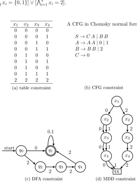
Example 2.3. Figure 2.4 gives examples for the table constraint, the CFG con-straint, the regular constraint, and the MDD constraint. The four 4-ary

con-straints are all dened on variables (x1, x2, x3, x4) with D(xi) = {0,1,2} for

i ∈ {1, . . . ,4}. Although the constraints have dierent representations, they are

in fact equivalent with the same semantics or relations c(x1, x2, x3, x4) ≡ [x1 =

0∧V4 i=2xi ={0,1}]∨[ V4 i=1xi = 2]. x1 x2 x3 x4 0 0 0 0 0 0 0 1 0 0 1 0 0 0 1 1 0 1 0 0 0 1 0 1 0 1 0 0 0 1 1 1 2 2 2 2

(a) table constraint

A CFG in Chomsky normal form:

S→C A|B B A→A A|0|1 B→B B |2 C→0 (b) CFG constraint 0 start 2 2 2 2 0,1 q0 q1 q2 q3 q4 (c) DFA constraint 0 0 1 0 1 1 0 2 2 2 2 x1 tt x2 x2 x3 x3 x4 x4 (d) MDD constraint

(33)

Chapter 3 GAC Algorithms for Regular

Constraints

Global constraints based on formal languages can be used to express arbitrary constraints including other global constraints. The most well known is perhaps the regular constraint [Pes04] which can also express other global constraints, e.g. contiguity [Mah02],among [BC94], lex[CGLR96], precedence[LL04], stretch [Pes01], etc. Theregularconstraint (originally) takes a deterministic nite automata (DFA) as the constraint denition but a non-deterministic nite automata (NFA) is also possible. On the other hand, the table constraint denes an arbitrary constraint explicitly as a set of solutions. Two ecient generalised arc consistency (GAC) algorithms for non-binary table constraints aremddc[CY10] and STR2 [Lec11]. In mddc, the constraint is specied as a multi-valued decision diagram (MDD) while STR2 works with the explicit table.

We see then that there can be many input representations dening the same set of solutions (tuples) to a constraint, though these representations may be regarded as dierent constraint forms with equivalent semantics. Moreover, it is well known that transforming an NFA to a DFA can lead to an exponentially larger automata. The MDDs corresponding to an NFA can also be large. Thus, there are dierent constraint representation choices with dierent space requirements for the associated GAC algorithms. Experiments in [Lec11] also show that the representation size can determine solver runtime, mddc is faster than STR2 when the MDD representation is more compact and vice versa.

In this chapter, we investigate the space-time tradeos of the NFA, DFA and MDD representations of the same equivalent constraint. Figure 3.1 gives a graph-ical representation of equivalent NFA, DFA, and MDD constraints. We extend mddc to nfac which can enforce GAC on a constraint dened either as an NFA, a

(34)

(a) (b) (c)

Figure 3.1: (a) an NFA and (b) an equivalent DFA (non-minimized). Each (dou-ble) circle with label i represents a (nal) state qi. There is a directed edge from

i to j i qj ∈δ(qi, a), where the edge is solid if a = 1 and dotted if a = 0. (c) an

equivalent MDD for a 4-ary regular constraint represented by the NFA in (a) or the DFA in (b).

DFA or an MDD. An algorithm which converts a constraint in NFA or DFA form directly to an MDD is also given.

We experiment with hard CSPs whose size dierences in their NFA, DFA and MDD representations are large. We show two space-time tradeos of nfac algorithm for regular constraints dened on these representations. First, the NFA representation is more ecient for the nfacalgorithm once the corresponding DFA or MDD becomes big enough. If memory itself is an issue, e.g. the CSP has many large constraints, it may be worthwhile to use NFA even when the DFA or MDD is smaller. Second, when the size of the DFA or MDD is large enough, once the total time including construction and initialization times are taken into account, the NFA can be much faster then DFA or MDD. We also compare nfac with regularc.

3.1 Overview of the GAC Algorithms for the

Reg-ular and MDD constraints

In this section, we introduce two GAC algorithms, one for theregularconstraint and one for the MDD constraint. To dierentiate the propagation algorithms from the

(35)

name of the constraints, we call the two existing GAC algorithms regularc [Pes04] and mddc [CY10] respectively. Similarly, in the following section, we name the proposed GAC algorithm for the NFA constraint, nfac. The regularc and mddc algorithms enforce GAC in dierent ways: regularc is ne-grained [LBH03] (incre-mental) that enforces GAC on the variable-value pairs, which results in a propaga-tion queue composed of variable-value pairs; whilemddcis coarse-grained [LBH03] (non-incremental) that enforces GAC on the constraints, which results in a prop-agation queue composed of constraints. An analog is that regularc is ne-grained like AC-4 [MH86], while mddc is coarse-grained like AC-3 [Mac77a].

3.1.1 The Filtering Algorithm for Regular Constraints

In this subsection, we review the GAC algorithm regularc introduced by Pe-sant [Pes04]. Assume that the regular constraint is dened on n variables, then regularc enforces GAC on a layered-graph withn+ 1layers{L0, . . . , Ln} of nodes.

The nodes of each layer correspond to the states in the automaton A, and the

arcs between nodes in the two adjacent layers corresponds to the arcs between the corresponding states of A. The execution of regularc is composed of a two-stage

forward and backward processing.

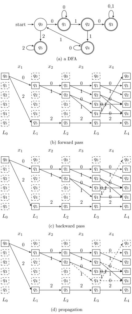
We use an example to show how the algorithms works. Figure 3.2(a) gives a DFA A of the regular (X, A) constraint, where X = {x1, . . . , x4} with domains

D(xi(16i64)) = {0,1,2}. The layered-graph is constructed initially by expanding Afrom the start stateq0 in a forward pass, giving the graph in Figure 3.2(b). The

nodes and arcs marked as solid are reachable from the start state q0 through a

sequence of valid values. The values corresponding to the solid arcs are treated consistent in this pass, but may be found inconsistent in the following pass. In the backward pass, the nodes and arcs that cannot lead to a nal state will be removed, as DFA only recognizes the sequence of values reaching to a nal state. In Figure 3.2(c), q0 ∈L4 is not a nal state; thus the incoming arc of it should be

removed. The values of the removed arcs will be removed from variables' domains if there are no other arcs with the same values that can lead to a nal state. Thus,

1 will not be removed from D(x4). The process terminates at Level L3 because

all nodes in this level can reach a nal state. After the initialization, value 1 is

removed from D(x1).

Then we introduce the value-based propagation with reference to Figure 3.2(d). Assume that 0 is removed from D(x4), then the arcs of (x4,0) will be removed.

The forward and backward pass update the graph using the removed arcs. The forward pass makes q1 ∈L4 unreachable and stops as L4 is the last layer. In the

(36)

backward pass,q4 ∈L3cannot reach any nal states; thus the incoming arc (x3,1)

of it will also be removed. As this arc is not the only out-coming arc of q2 ∈ L2,

the backward pass stops. Moreover, because (x3,1) has another supporting arc

linking q1 ∈L2 and q2 ∈L3,(x3,1)is still consistent. The propagation stops with

no inconsistent values found.

3.1.2 The Filtering Algorithm for MDD Constraints

Dierent from the regularc algorithm, the GAC algorithm, mddc [CY10], for the MDD constraint is coarse-grained. It seeks supports for the values of variables' domains by recursively exploring MDD from the root node to the terminal node. It keeps a data structureSifor each variablexito remember the values ofD(xi)for

which no supports are founded. Si is initially set as the domain of xi. Once an arc

with valuea ∈Si is found to be part of a path (composed of valid values) from the

root node to the true-terminal of the MDD, (xi, a) is GAC and can be removed

from Si. The values along the path correspond to a support of (xi, a). After

updating every Si, the values left in Si are inconsistent and should be removed

fromD(xi).

The mddc algorithm can be optimized from two directions. First, each node of an MDD may have more than one parent, hence may be accessed more than once during the exploration. Thus, the true and false semantics of each MDD node (dened in Section 2.4.4 which indicates whether the node can reach a true-terminal or not) can be recorded and reused in mddc. As a result, when an MDD node is accessed again, the truth of the sub-MDD rooted with this node can be returned instantly, rather than being recursively explored again. Furthermore, the semantics of MDD nodes can be used incrementally, which is inspired from the following observation: an inconsistent constraint will still be inconsistent when more variables are assigned in a CSP. For MDD, the false nodes will still be false when more variables are assigned. This can be implemented by using the sparse set data structure [BT93], which can give ecient restoration in backtrack search. Second, the setSi may be cleared before each path in the MDD is checked, so that

we can use a ag to remember the level at and below which all the values in the domains of the variables are consistent. This ag will help save more checks when seeking supports along the other paths. This is called the early-cuto optimization [CY06].

(37)

q0 start q5 q1 q2 q3 q4 2 0 2 1 0 0 1 0,1 0 1 (a) a DFA x1 x2 x3 x4 q0 q0 q0 q0 q0 q1 q1 q1 q1 q1 q2 q2 q2 q2 q2 q3 q3 q3 q3 q3 q4 q4 q4 q4 q4 q5 q5 q5 q5 q5 L0 L1 L2 L3 L4 0 2 2 1 0 2 1 0 1 0 2 1 0 0 1 0,1 0 1 (b) forward pass x1 x2 x3 x4 q0 q0 q0 q0 q0 q1 q1 q1 q1 q1 q2 q2 q2 q2 q2 q3 q3 q3 q3 q3 q4 q4 q4 q4 q4 q5 q5 q5 q5 q5 L0 L1 L2 L3 L4 0 2 2 1 0 2 1 0 1 0 2 1 0 0 1 0,1 0 1 (c) backward pass x1 x2 x3 x4 q0 q0 q0 q0 q0 q1 q1 q1 q1 q1 q2 q2 q2 q2 q2 q3 q3 q3 q3 q3 q4 q4 q4 q4 q4 q5 q5 q5 q5 q5 L0 L1 L2 L3 L4 0 2 2 1 0 2 1 0 1 0 2 1 0 0 1 0,1 0 1 (d) propagation

(38)

3.2 NFA-to-MDD Conversion

Since we want to investigate the performance of GAC algorithms on dierent representations, we may rst do a transformation between those representations, i.e. convert an r-ary NFA constraint into an equivalent MDD constraint. One

approach could be to rst construct a DFA from the NFA, e.g. by using the subset construction algorithm [Les95]. The DFA can then be traversed to generate solutions lexicographically which are then inserted into an MDD using the mddify construction algorithm [CY10]. However, the DFA may be exponentially larger than the NFA, in which case a DFA minimization may be used. Note that DFA minimization is PSPACE-hard in general [MS72].

In this section, we propose instead to convert directly from the NFA into the corresponding MDD constraint. More precisely, given an NFAG=hQ,Σ, δ, q0, Fi,

the algorithm nfa2mdd creates an MDD G0 = hQ0,Σ, δ, q₀0,{tt}i such that the r

-ary constraints represented by G and G0 are equivalent. The pseudo-code of the

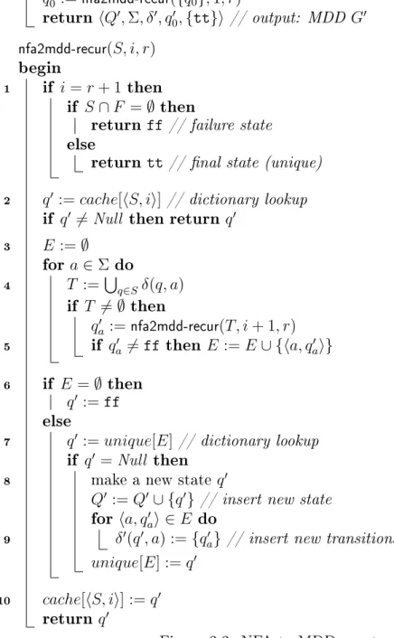
algorithm nfa2mdd is in Figure 3.3. The idea is to simulate the NFA [Tho68] in a depth-rst fashion and build the MDD in a bottom-up fashion. In other words, it combines NFA-to-DFA conversion (or subset construction) and trie-to-MDD construction.

We rst introduce the two dictionaries cache and unique that are used in nfa2mdd and nfa2mdd-recur. To save the NFA exploration, cache maps a pair of

hS, ii to a constructed MDD nodeq, where S is a set of NFA states, iis the

cur-rent level of the MDD. To construct reduced MDDs, unique maps one MDD node

q's all outgoing arcs to q itself.

The execution of the main procedurenfa2mdd-recur is as follows: If the current subsetSof states of the NFAGis at depthi=r+ 1(line 1), the unique nal state

tt of the MDDG0 is returned iS contains a nal state of G. This is because, by

denition, any path from the start state to a nal state corresponds to a solution of the NFA constraint i its length isr. Otherwise (i≤r), the traversal continues

by visiting collective successors for everya ∈Σ, the initial domain of the variable

(line 3). The recursive call returns the start state q0_a of the sub-MDD. If q_a0 is

not the failure state, the pair (a, q_a0) is recorded (line 5). Thus the MDD only

contains paths leading to tt (true). Now, if all successors of the states in S

lead to a dead-end, the failure stateff will be returned (line 6), which means the

current sub-MDD has no solution. Otherwise, we need to create a (new) start state for this sub-MDD. By denition, two equivalent (sub-)MDD constraints should be represented by the same sub-MDD, so we useunique, implemented as a dictionary,

(39)

can identify equivalent sub-MDDs easily by using E as a key (line 7). When we

cannot nd an existing state, we generate a new one (line 8) and the corresponding transitions (line 9).

nfa2mdd(G, r)

// input: NFA G=hQ,Σ, δ, q0, Fi and arity r

begin

Q0 :=∅

initialize cache[], unique[] // dictionaries

δ0 :=∅

q0₀ :=nfa2mdd-recur({q0},1, r)

return hQ0,Σ, δ0, q0₀,{tt}i // output: MDD G0 nfa2mdd-recur(S, i, r)

begin

1 if i=r+ 1 then

if S∩F =∅then

return ff // failure state

else

return tt // nal state (unique)

2 q0 :=cache[hS, ii] // dictionary lookup

if q0 6=Null then return q0

3 E :=∅ for a∈Σ do 4 T :=S q∈Sδ(q, a) if T 6=∅then q0_a:=nfa2mdd-recur(T, i+ 1, r) 5 if q_a0 6=ff then E :=E∪ {ha, q_a0i} 6 if E =∅ then q0 :=ff else

7 q0 :=unique[E] // dictionary lookup

if q0 =Null then 8 make a new stateq0

Q0 :=Q0∪ {q0} // insert new state

for ha, q_a0i ∈E do

9 δ0(q0, a) :={q_a0} // insert new transitions

unique[E] :=q0 10 cache[hS, ii] :=q0

return q0

(40)

Proposition 3.1. nfa2mdd-recur constructs reduced MDDs.

Proof. According to the algorithm, one stateqwill be generated only when there is

no other stateq0 that qandq0 have the same set of outgoing arcs. This guarantees

that no two dierent states q and q0 will be generated if q and q0 are isomorphic

and the MDD being constructed is reduced.

The depth-rst traversal will implicitly enumerate an exploration tree of size

|Σ|r_{. To reduce the size of the traversal, we make use of caching (lines 2 and}

10) to ensure that any sub-MDD will only be expanded once. In the worst case, nfa2mdd-recur visits O(2|Q|_r₎ _{NFA states. This is also the maximum number of}

slots in cache. However, the cache size can be smaller, thus trading time for

space. Note that if we convert an NFA into a DFA using subset construction the time complexity will be O(22|Q|) since the DFA will have at most O(2|Q|) states.

Given an NFA G = hQ,Σ, δ, q0, Fi and arity r, the runtime and space

com-plexities of nfa2mdd are given as follows:

Proposition 3.2. The worst-case time complexity of nfa2mdd is O(|Q|2 _{· |}_Σ_{| ·}

min{2|Q|_·_r,_|_Σ_|r+1_}₎.

Proof. In each call of nfa2mdd-recur, the caching operations on cache and unique

take O(|Q|) and O(|Σ|) time respectively. Every set union at line 4 can take

O(|Q|2₎_{time. The last term accounts for the maximum number of recursive calls:}

(1) each subset of Q is at most visited r times, and (2) the generation tree has O(|Σ|r₎ _{non-leaf nodes.}

In practice, the use of caching may signicantly reduce the runtime.

Proposition 3.3. The worst-case space complexity ofnfa2mdd isO(max{2|Q|_·|_Q_|·

r,|Σ|r_{· |}_Σ_|}₎_.

Proof. (1) for cache, the maximum number of slots is O(2|Q|_r₎ _{and for each slot,}

the keyStakesO(|Q|)space in the dictionary entry, and (2) forunique, the MDD

size is inO(|Σ|r₎_{and same as} _cache_{, each slot takes}_O₍_|_Σ_|₎ _space.

To reduce this high memory requirement, we can trade time for space and restrict the number of entries in cache and/or unique. In the latter case, the

resulting MDD may not be reduced and has more nodes, i.e., it may contain equivalent sub-MDDs.

Proposition 3.4. The output MDD G0 is in the worst case r times larger than

the DFA equivalent to the input NFA G, but it is exponentially smaller than the

(41)

Proof. For the worst case, suppose nfa2mdd is run on a DFA equivalent to G.

Since nfa2mdd-recur visits every DFA state at most r times, there will be at most r MDD states created for each DFA state. For the best case, consider an NFA

that represents the regular expression{0,1}∗₀_{₀_,₁_}n_{. The equivalent DFA has}₂n

nodes; whereas, for any xed r > n, the corresponding MDD has r+ 1 states,

which represents the constraint (xr−n = 0)∧

Vr

i=1xi ∈ {0,1}.

Thus, we suggest that the size of a DFA and MDD are not comparable with an NFA.

3.3 Maintaining GAC on NFA Constraints

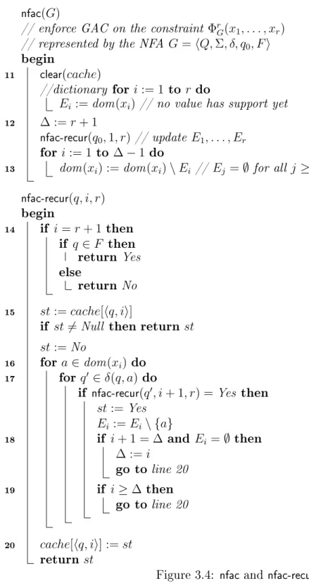
There are a number of approaches to enforce GAC on an NFA constraint. In this section, we propose an algorithm which generalizes themddcalgorithm [CY10] for MDD constraints to enforce GAC on NFA or DFA constraints. Figure 3.4 shows the algorithm nfac, which enforces GAC on an r-ary NFA constraint represented

by an NFA G=hQ,Σ, δ, q0, Fi. Thenfac algorithm can be applied to a constraint

represented in NFA, DFA or MDD, as a DFA or an MDD is a special case of an NFA.

Throughout the execution, for each xi, nfac keeps a set Ei of values in the

domain of xi which have no support (found yet). The function nfac-recurtraverses

G recursively and updates E1, . . . , Er on the y. Line 13 then removes for each

variable all values that have no support from its domain.

The function nfac-recur works as follows: If the current state q is at depth i =r+ 1 (line 14), Yes is returned i q is a nal state of G. This is because, by

denition, any path from the start state to a nal state corresponds to a solution of the NFA constraint i its length isr. Otherwise (i≤r), the traversal continues

for every a ∈ dom(xi) (line 16) and every q0 ∈ δ(q, a) (line 17). In the case of

a DFA or MDD, the set δ(q, a) only contains one state for a DFA so the loop at

line 17 will only be executed once.

Then if nfac-recurreturns Yes, we will remove a fromEi because (xi, a)has at

least one support. Line 18 and 19 terminate the (outermost) iteration as soon as every value in every domain of xi, xi+1, . . . , xr has a support. This is called

the early-cuto optimization and it avoids traversing parts of the explored graphs. At last the function returns st, which is Yes if the current sub-NFA constraint is satisable and No otherwise.

Proposition 3.5. When nfac-recurterminates, the value a∈Ei i the assignment

(42)

nfac(G)

// enforce GAC on the constraint Φr

G(x1, . . . , xr)

// represented by the NFA G=hQ,Σ, δ, q0, Fi

begin

11 clear(cache)

//dictionary for i:= 1 to r do

Ei :=dom(xi) // no value has support yet

12 ∆ :=r+ 1

nfac-recur(q0,1, r) // update E1, . . . , Er

for i:= 1 to ∆−1do

13 dom(xi) := dom(xi)\Ei // Ej =∅ for all j ≥∆

nfac-recur(q, i, r) begin 14 if i=r+ 1 then if q ∈F then return Yes else return No 15 st:=cache[hq, ii]

if st6=Null then return st st:=No

16 for a∈dom(xi) do

17 for q0 ∈δ(q, a)do

if nfac-recur(q0, i+ 1, r) =Yes then

st:=Yes Ei :=Ei\ {a} 18 if i+ 1 = ∆ and Ei =∅ then ∆ :=i go to line 20 19 if i≥∆ then go to line 20 20 cache[hq, ii] :=st return st

Figure 3.4: nfac and nfac-recur.

Proof. As discussed above, all values a that have supports are removed from Ei.

The use of caching at lines 15 and 20 guarantees nfac-recurtraverses each sub-NFA at most r times. The entries in cache are emptied by the procedure clear

(43)

the sparse set data structure used in mddc [CY10].

Given an NFA G = hQ,Σ, δ, q0, Fi and arity r, we have the following results

on the runtime and space complexity of nfac.

Proposition 3.6. The time complexity of nfac is O(|δ| ·r).

Proof. With caching, each state in G is visited O(r) times, and the two for-loops

at line 16 traverse each outgoing edge of the state at most once (operations on

cachetakes O(1) time [CY10]).

Proposition 3.7. The space complexity of nfac is O(|δ|+|Q| ·r) if the cache is

maximal.

Proof. The rst term corresponds to the number of transitions inGand the second

term gives the space requirement for cache(each entry in cachetakes O(1) space

[CY10]).

However, if the cache has a xed size, the space complexity becomes O(|δ|). This

suggests a possible tradeo between time and space by tuning the maximum size of cache.

3.4 Experiments

Our implementations are in C++. The MDD construction with nfa2mdd is im-plemented with the STL library for convenience. As STL is not so ecient, we can expect that the runtime can be further improved but still the trends from the experiments below are clear. We implement nfac in Gecode 3.5.0 as it has an ecient implementation of regularc [Pes04]. The cache implementation in nfac

follows [CY10] using a sparse set [BT93] (for fast incrementality). Experiments were run on an Intel i7/960 @3.20GHz with 12G RAM on 64-bit Linux. We use FSA Utilities 6.276 [vN], implemented in Prolog, to do the NFA generation and dk.brics.automaton [Bri], implemented in Java, to do DFA determinization and minimization.

We want to investigate time-space tradeos, so that the benchmarks need to: (i) have sucient variation in size between NFA, DFA and MDD representations; and (ii) be suciently hard with the chosen search heuristic so that we are able to adequately exercise the GAC algorithms. Existing benchmarks do not meet our goals, e.g. structured problems do not have variant sizes. We thus chose to generate hard random CSPs for these goals using NFA constraints. We generate