Implementing the BG/NBD Model for
Customer Base Analysis in Excel
Peter S. Fader www.petefader.com Bruce G. S. Hardie www.brucehardie.com Ka Lok Lee† www.kaloklee.com June 2005 1. Introduction
This note describes how to implement the BG/NBD model for customer base analysis1 using Microsoft Excel. There are three key stages to the implementation of this model:
1. estimating the model parameters,
2. generating the aggregate sales forecast given these parameter esti-mates, and
3. predicting a particular customer’s future purchasing, given information about his past behavior and the parameter estimates.
The specific steps are outlined in sections 3–5 below. Section 2 briefly de-scribes the nature of the data used for model calibration. All these sections
should be read in conjunction with the Excel workbook bgnbd.xls. (We
strongly encourage interested readers to build the spreadsheet that imple-ments the model “from scratch” for themselves, using this note and the
Excel workbookbgnbd.xls as a guide.)
†c 2004, 2005 Peter S. Fader, Bruce G. S. Hardie, and Ka Lok Lee. This note and the
associated Excel workbook can be found at <http://brucehardie.com/notes/004/>. This research was supported in part by ESRC grant R000223742 (awarded to Bruce G. S. Hardie).
Cus-2. Data
The model requires three pieces of information about each customer’s past purchasing history:his “recency” (when his last transaction occurred), “fre-quency” (how many transactions he made in a specified time period), and the length of time over which we have observed his purchasing behavior. The notation used to represent this information is (X = x, tx, T), where
x is the number of transactions observed in the time period (0, T] and tx (0< tx≤T) is the time of the last transaction.
The worksheet Raw Data contains these data for a sample of 2357 CD-NOW customers who made their first purchase at the web site during the first quarter of 1997. We have information on their repeat purchasing be-havior up to the end of week 39 of 1997.
While the basic unit of time is one week, we recognize that transactions can occur on each day of the week. Therefore consider customer 0001 (row 2). The number of days (in weeks) during which repeat transactions could have occurred isT = 38.86, which implies this customer made his first-ever purchase at CDNOW on the first day of the first week of 1997. Over this time period, this customer madex= 2 repeat purchases, with the second repeat purchase occurring on the third day of the 30th week of 1997 (tx = 30.43). Scrolling down the worksheet, we notice that most customers (1411 in total) had not made a repeat purchase (x= 0) by the end of week 39.
3. Calibrating the BG/NBD Model
We start by making a copy of the Raw Dataworksheet — let’s call it BGNBD Estimation— and inserting six rows at the top of the worksheet. Our goal is to construct the log-likelihood function — as given in equations (6) and (7) of the paper — and find the values of the model parameters associated with its maximum value.
First we need to enter the expression for lnL(r, α, a, b|X = x, tx, T) for each of the 2357 customers in the sample. In order to create the corre-sponding expression in the worksheet without an error message appearing (e.g.,#NUM!or#DIV/0!), we need some “starting values” for the four model parameters. The exact values do not matter — provided they are within the defined bounds — so we start with 1.0 for r, α, a, and b. We locate these parameter values in cellsB1:B4.
As noted on p. 280 of the paper, the likelihood function for a randomly-chosen individual with purchase history (X=x, tx, T) can be written as
where A1 = Γ(r+x)α r Γ(r) A2 = Γ(a+b)Γ(b+x) Γ(b)Γ(a+b+x) A3 = 1 α+T r+x A4 = a b+x−1 1 α+tx r+x and δx>0 = 1 if x >0, 0 otherwise. This is easy to “code up” in Excel:
• The log ofA1 is simply lnΓ(r+x)−lnΓ(r)+rln(α). The formula in cellF8is the expression of this for the first customer:
=GAMMALN(B$1+B8)-GAMMALN(B$1)+B$1*LN(B$2)
• The log ofA2 is lnΓ(a+b)+lnΓ(b+x)−lnΓ(b)−lnΓ(a+b+x), which is entered in cellG8 for the first customer as
=GAMMALN(B$3+B$4)+GAMMALN(B$4+B8)-GAMMALN(B$4) -GAMMALN(B$3+B$4+B8)
• The log ofA3 is −(r+x)×ln(α+T), which is entered in cell H8 for the first customer as
=-(B$1+B8)*LN(B$2+D8)
• The log ofA4 is ln(a)−ln(b+x−1)−(r+x)×ln(α+tx). We should only compute this if x > 0; should x = 0 and b be < 1, we would end up taking the log of a negative number. We therefore enter this expression in cellI8for the first customer as
=IF(B8>0,LN(B$3)-LN(B$4+B8-1)-(B$1+B8)*LN(B$2+C8),0)
• Finally, a single customer’s contribution to the sample log-likelihood function is
lnL(r, α,a, b|X=x, tx, T)
= ln(A1) + ln(A2) + ln(A3+δx>0A4)
= ln(A1) + ln(A2) + lnexp(ln(A3)) +δx>0 exp(ln(A4)), which is entered in cellE8 for the first customer as
=F8+G8+LN(EXP(H8)+(B8>0)*EXP(I8))
The sum of cells E8:E2364 is found in cell B5; this is the value of the log-likelihood function — equation (7) of the paper — as evaluated at the specific values of the four model parameters in cellsB1:B4. (With starting values of 1.0 for all four parameters, LL=−13887.7.)
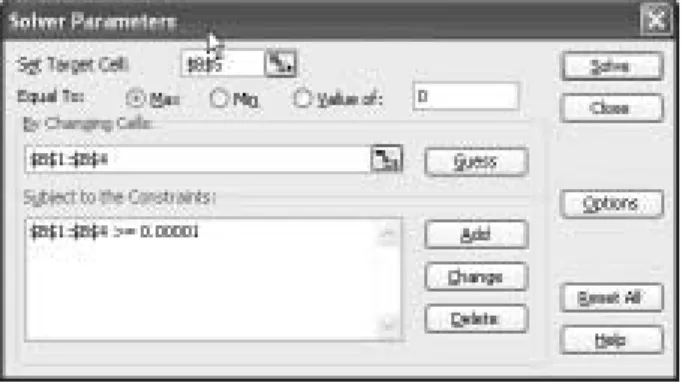
Given these sample data, we find the maximum likelihood estimates of the four model parameters by maximizing the log-likelihood function. We do this using the Excel add-in Solver, available under the “Tools” menu. The
target cell is the value of the log-likelihood (cell B5); we wish to maximize
this by changing cells B1:B4. The constraints we place on the parameters are thatr,α,a, andbare greater than 0. As Solver only offers us a “greater than or equal to” constraint, we add the constraint that cells B1:B4 are ≥ a small positive number (e.g., 0.00001). (See Figure 1.) Clicking the Solve
button, Solver finds the values of the four model parameters that maximize the log-likelihood function.
Figure 1:Solver Settings
But can we be sure that we have reached the maximum of the log-likelihood function? Using the solution given by Solver as the set of starting values for the parameters, we “fire up” Solver again to see if it can improve on this solution. Once we are satisfied that the maximum has indeed been reached, we can say that the numbers given in cellsB1:B4are the maximum likelihood estimates of the model parameters. As reported in Table 2 of the paper, the maximum value of the log-likelihood function is −9582.4, associated withr= 0.243, α= 4.414,a= 0.793, andb= 2.426.
So as to be sure that these are indeed the maximum likelihood estimates of the model parameters, it is good practice to redo the optimization process using a completely different set of starting values. For example, using start-ing values of {0.01, 0.01, 0.01, 0.01} for cells B1:B4, repeatedly use Solver until you are satisfied that the maximum of the log-likelihood function has been reached. Are the corresponding values of the four model parameters equal to those given above? (They should be!)
4. Creating the Sales Forecast
Now that we have estimates of the four model parameters, we can turn our attention to the task of creating a forecast of repeat purchasing by the cohort of 2357 customers.
For a randomly-chosen individual, the formula for computing the ex-pected number of transactions in a time period of lengthtis
E(X(t)|r, α, a, b) = a+a−b−11 1− α α+t r 2F1r, b;a+b−1;α+tt, (1) where 2F1(·) is the Gaussian hypergeometric function. In the worksheet
E{X(t)}, we compute this quantity for each day up to the end of week 78 (our forecast horizon); thust= 1/7,2/7, . . . ,78 (cells A7:A552).
Central to equation (1) is the Gaussian hypergeometric function, which is the power series of the form
2F1(a, b;c;z) = ∞ j=0 (a)j(b)j (c)j zj j!, c= 0,−1,−2, . . . ,
where (a)j is Pochhammer’s symbol, which denotes the ascending factorial
a(a+ 1)· · ·(a+j−1). (Note that an ascending factorial can be represented as the ratio of two gamma functions, (a)j = Γ(a+j)/Γ(a).) The series converges for |z| < 1 and is divergent for |z| > 1; if |z| = 1, the series converges forc−a−b >0. Writing 2F1(a, b;c;z) = ∞ j=0 uj, where uj = (a()cj)(b)j j zj j!
we have the following recursive expression for each term of the series:
uj
uj−1 =
(a+j−1)(b+j−1)
(c+j−1)j z , j= 1,2,3, . . .
whereu0 = 1.
This lends itself to a simple (and relatively robust) numerical method for the evaluation of the Gaussian hypergeometric function:continue adding terms to the series untiluj is less than “machine epsilon” (the smallest num-ber that a specific computer recognizes as being bigger than zero). How-ever, when “hard-coding” this in a worksheet (as opposed to, say, creating a custom function using VBA), it is easier to compute the series to a fixed number of terms; in this case, we will evaluate the first 151 terms (i.e.,
Let us consider the first time point,t= 1/7 (row7). Looking at equation (1), the ‘z’ argument of the Gaussian hypergeometric function is t/(α+t); this is given in cellD7. Starting at cellE7, we compute each term of the series forj = 0, . . . ,150. (The values of the indexj are given in cellsE6:EY6.) As noted above, the value of u0 is 1 (cellE7). To compute the value of u1, we multiplyu0 by
(a+j−1)(b+j−1)
(c+j−1)j z
where, looking at equation (1), ‘a’ is the BG/NBD model parameterr, ‘b’ is the BG/NBD model parameterb, ‘c’ equals the BG/NBD model parameters
a+b−1, the value of ‘z’ is given in cellD7, andj = 1. The Excel formula used to computeu1 is therefore
=E7*$D7*($B$1+F$6-1)*($B$4+F$6-1)/(($B$3+$B$4-1+F$6-1)*F$6)
We copy this formula across to cell EY7, which corresponds to j = 150. Summing these terms gives us the numerical value of the Gaussian hyper-geometric function for this set of function parameters (cellC7).2
The computation of E[X(t))] follows naturally in cellB7; the Excel for-mula associated with equation (1) is simply
=(B$3+B$4-1)/(B$3-1)*(1-(B$2/(B$2+A7))ˆB$1*C7)
Having created values oftup to 78 in day increments (cellsA8:A552), we copy the block of cells (B7:EY7) down to row 552. We have now computed the value ofE[X(t)] day-by-day to the end of our 78-week forecast horizon (cells B7:B552).
However, we are not interested in the expected number of repeat transac-tions for a randomly-chosen individual; rather we are interested in tracking (and forecasting) the total number of repeat transactions by the cohort of customers. In computing this cohort-level number, we need to control for the fact that different customers made their first purchase at CDNOW at different points in time during the first quarter of 1997, and consequently differ in the length of the time period during which they could have made re-peat purchases. Given our recognition that transactions can occur on each day of the week, we need to consider 7×12 = 84 different first-purchase dates.
Total repeat transactions can be computed as follows: Total Repeat Transactions by t=84
s=1
δ(t> s
7 )nsE[X(t− s
7)] (2) 2In terminating the series atj= 150, have we evaluated too many or too few terms?
Looking at the matrix ofuj terms in the worksheetE{X(t)}, we see that the speed with
whichuj→0 depends on the magnitude ofz. In this particular case, there is no point in
going beyondj= 40 forz <0.5. However we should probably be evaluating more terms forz= 0.94, sinceu150= 1.39E−06 is still some distance from “machine epsilon”.
wherens is the number of customers who made their first purchase at
CD-NOW on day s of 1997 (and therefore have t− s7 weeks within which to
make repeat purchases) andδ(t> s
7 )= 1 if t > s
7, 0 otherwise.
We determine the values ofnsin the worksheetn s. GivenT, the number of days (in weeks) during whichrepeat transactions could have occurred in the 39-week calibration period (column B), it follows that the time of the first purchase is simply 39−T (columnC). Performing a pivot table analysis yields the number of customers who made their first purchase on each of the 84 days of the first quarter that defines this cohort of customers.
Equation (2) is evaluated for t = 1/7,2/7, . . . ,78 via the block of cells
E1:CM549 in the worksheet Cum Rpt Sls. Cells B4:B81 report the cumu-lative number of repeat transactions for each of the 78 weeks (using the
=OFFSET()function to “pick out” the relevant numbers from columnF. The expected number of weekly repeat transactions are reported in cellsC4:C81. Some readers may be questioning the numerical precision of these fore-casts, given our relatively crude method for evaluating the Gaussian hyper-geometric function. These same forecasts were computed in MATLAB using a more refined implementation of the numerical method outlined above to evaluate the Gaussian hypergeometric function — one in which the series ter-minates when the next term (uj) is less than machine epsilon, instead of at
a fixed point (j = 150 in our spreadsheet implementation). The maximum
percentage difference between the two sets of cumulative repeat transaction numbers (across the 78 weeks) is 0.01% and by the end of the week 78, the forecasts differ by 0.40 of a transaction. We feel that these deviations are tolerable.
5. Computing Conditional Expectations
Finally, we turn our attention to the task of predicting a particular cus-tomer’s future purchasing, given information about his past behavior and the parameter estimates. The expression used to compute this quantity is
E(Y(t)|X=x, tx, T, r, α, a, b) = a+ba+−x1−1 × 1− α+T α+T+t r+x 2F1r+x, b+x;a+b+x−1;α+Tt+t 1 +δx>0b+xa−1 α+T α+tx r+x , (3)
which we implement in the worksheetConditional Expectation.
We start by placing our estimates of the four model parameters in cells
specifyt, the length of the period over which we wish to make the conditional forecast (cellB9).
Let us perform this calculation for the first customer in our dataset (ID = 0001), who made his first purchase on the first day of the first quarter of 1997 (and therefore hadT = 38.86 weeks within which he could make repeat transactions). During this period, he made x = 2 additional transactions at the CDNOW web site, with the last transaction occurring on the third day of week 30 (tx = 30.43). We wish to compute the expected number of transactions in weeks 40–78 (i.e.,t= 39).
Central to equation (3) is the Gaussian hypergeometric function. We evaluate it using the method outlined in Section 4. The function parameters (a, b, c) are given in cells E2:E4 and the function argument (z) in cell E5. Once again, we evaluate the first 151 terms of the series (cells E7:E157)
and the sum of these terms is reported in cell E1. The computation of
E(Y(t)|X=x, tx, T) follows naturally in cellC11.
We would therefore expect this customer to make 1.2 transactions across weeks 40–78. We can make such calculations for other customers by entering their specific purchase histories (X =x, tx, T) and the forecast horizon (t) in cells B6:B9; the forecast of their expected future transaction levels will appear in cellC11.