For further information about ILLC-publications, please contact Institute for Logic, Language and Computation
Universiteit van Amsterdam Science Park 904 1098 XH Amsterdam phone: +31-20-525 6051 fax: +31-20-525 5206 e-mail:[email protected] homepage:http://www.illc.uva.nl/
ACADEMISCH
PROEFSCHRIFT
ter verkrijging van de graad van doctor aan de
Universiteit van Amsterdam
op gezag van de Rector Magnificus
prof.dr. D. C. van den Boom
ten overstaan van een door het college voor
promoties ingestelde commissie, in het openbaar
te verdedigen in de Aula der Universiteit
op dinsdag 9 maart 2010, te 14.00 uur
door
Jonathan Alexander Zvesper
geboren te Norwich, Verenigd Koninkrijk
Promotor: prof.dr. K.R. Apt
Promotor: prof.dr. J.F.A.K. van Benthem Overige leden:
dr. Alexandru Baltag prof.dr. Jan van Eijck
prof.dr. Peter van Emde Boas prof.dr. Dov Samet
prof.dr. Frank Veltman dr. Yde Venema
prof.dr. Rineke Verbrugge
Faculteit der Natuurwetenschappen, Wiskunde en Informatica Universiteit van Amsterdam
Science Park 904 1098 XH Amsterdam
Research supported by the ‘research training host fellowship’ GLoRiClass of the Eu-ropean Commision, MEST-CT-2005-020841.
Copyright c2010 by Jonathan A. Zvesper
Cover design by the author based on a photograph by Alessandra Lombardo. Printed and bound by Copytech (UK).
Acknowledgements vii
Introduction 1
1 Believing Rationality in Arbitrary Games 11
1.1 Strategic games and optimality operators . . . 14
1.2 Heuristic treatment . . . 26
1.3 Common belief in rationality . . . 31
1.4 Transfinite mutual belief in rationality . . . 41
2 Syntax and Interaction 57 2.1 Features of the syntactic approach . . . 59
2.2 Languages . . . 63
2.3 Complete models . . . 82
3 Dynamics 99 3.1 Dynamic epistemic logic . . . 102
3.2 Epistemic actions on games . . . 117
3.3 Belief revision and lexicographic rationality . . . 123
4 Extensive Games 135 4.1 Games with perfect information . . . 137
4.2 Conditions for backward induction . . . 145
4.3 Games with imperfect information . . . 160
Summary 175
Bibliography 179
Abstract 191
“[R]ationality of thought imposes a limit on a person’s concept of his relation to the cosmos” – John F. Nash Jr., [1995]
Krzysztof Apt and Johan van Benthem have had the unenviable task of advising a regularly un-punctual and sometimes humourless sloppy thinker for three years. It is difficult to imagine how they managed to do this, but to do so while still being willing to talk to me, and indeed to offer outstanding advice comments and criticism, requires further leaps. I thank them for generously sharing their ideas and synergistic perspectives on the topics covered here and beyond; for their immense patience; and for so many inspiring meetings.
Thanks also to all my committee members; everybody who sent comments sent some very useful comments, to which I hope to have done justice in the subsequent revisions. Additional thanks to Alexandru Baltag for all of our discussions, and for his support and encouragement.
I’d like to thank the instigator, participants, invited speakers and co-organisers of the various Palmyr workshops.1
Many people made the ILLC such a great place to work and play, I owe you all something, and to many of you much. I am grateful to Krister Segerberg and Eric Pacuit, as well as my supervisors, for teaching me some of the, by their stan-dards doubtless fairly elementary, mathematical skills required to write this thesis. For the especially good times, academic and otherwise, I offer my acknowledgements to Olivia Ladinig, C´edric D´egremont, Ga¨elle Fontaine, Raul LeaL, Am´elie Gheerbrant, Andi Witzel, Witzel Yun Qi, Simon Pauw, Umberto Grandi, Sujata Ghosh, Jacob Vos-maer, Nina Gierasimczuk, Jakub Szymanik, Henrik Nordmark, Daisuke Ikegami, Ren´e Goedman, Reut Tsarfaty and Joel and Sara Uckelman. Wouter (Koolen-Wijkstra): be-dankt voor de op-het-laatste-moment samenvatting!
1http://www.illc.uva.nl/PALMYR
over other projects. Danda provided the photograph on which the front cover’s image is based, and wonderful energy. everyone at Camp Busted, and Carla and Dannette, helped keep me relatively sane during the penultimate writing stages. Nadia didn’t-dance one Sunday morning. Louis, Thomas, Emma and Brad are the best imaginable sibling-like family members. And I am grateful to my parents for each selflessly doing so much for me.
Oxford, J. A. Z.
January 2010.
“We don’t have much left to do, we British, except to play our games”– Methwold [Rushdie, 1981]
Allow me to retain for a few more sentences a chatty tone, and the first person. Taking a step back from this Thesis, there is so much more I would have liked it to be, so let us say, while also retaining a down-to-earth sense of proportion, that it is aimed towards a theory of interactive reasoning. Game theory is for the most part the object of its study, and with good reason: game theory isall aboutinteraction. But game theory needn’t have a monopoly here. Computer scientists and philosophers are increasingly studying aspects of interaction too, with some formality [D´egremont and Zvesper, 2010], and something this thesis does is bring some aspects of their common ground –logic– to the fore.2 We’re still in chatty mode (just wait until you get to Chapter 1 if you want
to see what ‘dry’ means), so we’re allowed to admit some weaknesses. Sometimes we will get ‘bogged down’ in details of the particular disciplines we’re writing about. We prove certain Propositions and Theorems that might leave people cold, and our discussion could sometimes seem wide of the mark. People from game theory will say, ‘reduction axiom what now?’, and people from logic might wonder why we care about ‘players’ (as in real players, not ∀belard and ∃loise). Still, bear in mind that we’re contributing to something interdisciplinary here, all with the hope that justone truly interesting idea about interactive reasoning will eventually be squeezed out of the confusion.
In this Introduction we will first present, with minimal technical baggage or ma-chinery, the sort of things that are discussed in the following Chapters. So we talk a bit about game theory, and then about interactive epistemology (slipping in a little bit of logic). Those few pages arenotintended as a guide for the details of what is in the
2A shift of focus to interaction can be said to have been brewing for several decades, as a concerted
effort to change the fact that “[t]raditional philosophy of language, like much traditional philosophy, leaves out other people and the world” [Putnam, 1975, p. 193].
rest of this Thesis, but rather to whet the (relatively) lay reader’s appetite. We will also explain the so-called ‘deductive’ interpretation of game theory that we will principally have in mind throughout this Thesis, and give some reasons why we prefer to take ‘be-lief’ rather than ‘knowledge’ as the object of (interactive) epistemology. Then, after we’ve mentioned a few things we find interesting from the fields of game theory and interactive epistemology, we do endeavour to explain some of that will occur in the Chapters, one by one.
Game theory
Game theory is the mathematical study of the interactions of largely idealised decision-makers. Mathematical in the following sense: it abstracts from much of the detail of those interactions qua events taking place in the real world (which “might better be called the complex world” [Aumann, 1985]). The advantage to such an abstraction being that game theorists can present formal models, about which they can prove the-orems. These theorems, in turn, are supposed to tell us something about the complex world we abstracted away from.
To quote from the opening passage of a popular textbook on game theory [Osborne and Rubinstein, 1994],
“The basic assumptions that underlie [game] theory are that decision-makers pursue well-defined exogenous objectives (they arerational) and take into account their knowledge or expectations of otherdecision-makers’ behaviour (theyreason strategically).”
The Thesis you are reading uses formal tools drawn principally from work in philo-sophical logic to explore both of these notions,rationalityandstrategic reasoning, fo-cusing especially on the role of information and belief: on what are called ‘epistemic’ or sometimes ‘doxastic’ aspects.
Rationality here is taken to mean ‘instrumental’ rationality, i.e. rationality means just that players pursue their objectives, that can be taken to represent their ‘best in-terests’, as perceived by themselves. Players therefore function as optimisers ofwhat they take to betheir own best interests. There is a doxastic component therefore in the definition of this most fundamental notion in game theory:
“A person’s behaviour isrationalif it is inhisbest interests, givenhisinformation.”
That is the standard definition of (instrumental) rationality; the particular quotation is from [Aumann, 2006].
Perhaps the most widely known example of a game (in the sense of game theory) is the so-called “prisoner’s dilemma”. One formulation, from [Osborne and Rubinstein, 1994, p. 16], of the prisoner’s dilemma is the following:
Two suspects in a crime are put into separate cells. If they both confess, each will be sentenced to two years in prison. If only one of them confesses, he will be freed and used as a witness against the other, who will receive a sentence of three years. If neither confesses, they will both be convicted of a minor offence and spend one year in prison.
We will not introduce formally the definitions of games, including of players’ pref-erences (or ‘utilities’), until Chapter 1, but for present purposes allow us to represent the situation using the matrix in Figure 1. This matrix represents what we will call a
Y N
Y 1,1 3,0
N 0,3 2,2
Figure 1: A matrix representing the prisoner’s dilemma game
‘strategic game’; the important point about it is that it is intended to capture the es-sential parts of the given description of the situation the players (the prisoners) find themselves in. One player (the ‘row player’) must choose between the top and bot-tom rows, and the other (the ‘column player’) must choose between the left and right columns. The numbers in the resulting entry in the matrix (e.g.0,3) then represent the ‘utility’ obtained by the row and column players respectively. The choiceY (the top row for the row player; left column for the column player) represents confessing to the crime; the choice N represents not confessing.3 The utilities written in the boxes are made on the assumption that the only concern the players have is how much time they will spend in prison: 0 means spending three years in prison,1 means spending two years, etc.
Players prefer higher utilities, which means that in this case mainstream game the-ory makes a unique prediction: both players will playD, i.e. both players will confess. However, there are two ways to think about that prediction, which rely respectively on the ‘deductive’ and the ‘steady-state’ interpretations in game theory (cf. [Osborne and Rubinstein, 1994, Section 1.5]). Thedeductive interpretation will suit this sce-nario better; it says that a game matrix really represents a ‘one-shot’ interaction, in which players use only reasoning about the game, with no exogenous information. According to the deductive interpretation, players can perform the following kind of reasoning. The row player can say, ‘if my fellow prisoner playsY then I would be bet-ter off playingY; and if my fellow prisoner playsN then I would be better of playing Y; so I should playY’. ThusN is, to use game-theoretic jargon that we introduce in Chapter 1, ‘strictly dominated’ byY.
Thesteady-state interpretationof game theory is very different, and is the interpre-tation that supports the notion of ‘Nash equilibrium’. A Nash equilibrium is a ‘profile’
3These ‘confessions’ need not be sincere, as nothing in the scenario says whether or not the suspects
of strategies, i.e. one strategy for each player, such thatgiventhat those strategies are played, no player has an incentive to deviate from the profile. To put it otherwise, a Nash equilibrium is a best response to itself. In the prisoner’s dilemma, the unique Nash equilibrium is again where both players playY. – In any other entry in the ma-trix (i.e. in any other profile) at least one player has an ‘incentive’ to deviate from that profile. However, in a great many other games, the steady-state interpretation yields very different answers from the deductive interpretation.
For example, in so-called ‘pure coordination games’ like that in Figure 2, the de-ductive interpretation cannot make any prediction, since L and R are symmetric for both players. However, only(L, L)and(R, R)are Nash equilibria. From the point of
L R
L 1,1 0,0
R 0,0 1,1
Figure 2: A pure coordination game
view of the deductive interpretation then, the steady-state interpretation makes some kinds of additional assumptions, that arguably should be integrated into the description of the game. The steady-state interpretation is sometimes taken to assume tacitly some notion ofrepetitionof the scenario being represented.4 However, repetition itself
sub-stantively changes the game5. So perhaps communications or signals of some kind, for
example those underlying Aumann’s [1974] notion of correlated equilibrium, might be the best way to understand the steady-state interpretation of game theory.
Our interest almost throughout this work will be focused on the conceptually clearer deductiveinterpretation of game theory. So we in general have in mind a ‘one-shot’ kind of interaction, in which any repetition or communication should be modelled ex-plicitly as part of the game. (Furthermore, let us remark that we will not have anything to say about cooperative game theory.) Within the deductive interpretation, we will look at ‘interactive epistemology’, that is reasoning aboutbeliefs, including about be-liefs concerning bebe-liefs.
Formal interactive epistemology
Alongside mathematical structures that represent the games themselves, we will con-sider mathematical structures that are intended to formalise the notion ofinformation
4Sometimes the assumption is made more more explicit: “as a given setting gets more and more
common and familiar, it makes [the players] act more and more rationally in that setting” [Aumann, 1985].
5The observation that anarbitrarily repeated prisoner’s dilemma yields a different outcome was
orbelief, and so to get a handle on this talk of strategic reasoning, and indeed of ra-tionality. These structures, or ‘models’, represent “knowledge or expectations” of the players.
There is more to rationality and to strategic reasoning than simply having expec-tations about other players’ behaviour. Those expecexpec-tations themselves, e.g. playeri’s beliefs about what playerj will do, are often derivable from, and must at least be con-sistent with, some more fundamental beliefs of playeri. For instance player imight herself make the “basic assumption” mentioned in the quotation from Osborne and Rubinstein, so that i would in particular believe (since it follows from her “assump-tion”) that player j is rational and reasons strategically, perhaps based on a similar assumption.
We prefer to use the term ‘belief’ rather than ‘knowledge’ for a number of reasons. Firstly, we sometimes want to allow for the information the players have to be incor-rect. (Or if information has by definition to be correct, then we are allowing for what the playersthinkis their information to be incorrect.) Furthermore, we prefer the con-ceptual position which holds that given that the game itself somehow represents ‘real’ possibilities, the players do notknowof any of the possibilities that it will not occur: if youknowthat your opponent will not play a certain move, then arguably that move should not be included.6 Using the terminology of Brandenburger [2007], we take a
belief-based approachto game theory, that he outlines as follows:
“[O]nly observables are knowable. Unobservables are subject to belief, not knowledge. In particular, other players’ strategies are unobservables, and only moves are observables.” (op.cit., p. 489)
However, this choice of ours need not be taken to reflect any deep philosophical or epistemological point, and much of what we say about belief will also hold for knowledge. One almost indisputable property of knowledge, that clearly distinguishes it from belief, is that it is a ‘factive mental state operator’ [Williamson, 2000]: that if one knows something, then it is true. Plato’s definition of knowledge, as justified true belief, has been shown to be wanting by Gettier’s famous counterexamples, but it is certainly not controversial to maintain that it is a necessary condition, for a belief to be knowledge, that it be true.
If we were to insist that all beliefs modelled were true, perhaps we could call them ‘knowledge’. Indeed, if the reader particularly likes the term ‘knowledge’, and is un-persuaded by the above-cited view of Brandenburger, then she can substitute it for ‘true belief’ wherever she likes. Most of the results that we establish for belief hold for always-true belief and so, for such a reader, for knowledge. (Indeed everything in Chapters 1 and 2 holds reading ‘knowledge’ in the place of ‘true belief’; Chapters 3 and 4 make more fundamental use of the belief-based approach.)
A formal logical approach to studying the notions of knowledge and beliefs was instigated by Hintikka [1962], using so-called ‘modal logic’. And game theorists, most
6To fully motivate this line of argument we would have to say that if there is ‘common knowledge’
notably Aumann [1976], have independently developed formal models for knowledge and beliefs along the same lines.
Some crucial limitations to Hintikka’s work have since been overcome. For exam-ple, Hintikka writes that “I do not know how to characterize the notion of occasion exhaustively” (op.cit., p. 7), whereas the semantics that were soon to be developed for modal logic (pre-empting the epistemic models introduced in the game-theoretical literature) furnish precisely such a characterisation. The logical approach, and the knowledge and belief models proposed in the game theory literature, were for a long time what we will call ‘static’. That is, “[t]here cannot be any question of increasing one’s factual knowledge”; what is more, the only assertions about beliefs or knowledge that are susceptible to the formal analysis proposed there are those “made onone and the same occasion” ([Hintikka, 1962]). Yet Sorensen [2009] is able to write that
“just as it is easier for an Eskimo to observe an arctic fox when it moves, we often get a better understanding of the knower dynamically, when he is in the process of gaining or losing knowledge.”
Even if that quotation does describe the situation a little too colourfully (metaphorically speaking), still thechangeof beliefs and knowledge is an important phenomenon, and we will relate it to our study of games.
An important concept in interactive epistemology is that of ‘common knowledge’, which we can think of as a special case of ‘common belief’. A fact is commonly believed (by a group) if everybody (in that group) believes it, they all believe that they all believe it, and so on. (Actually we will see in Chapter 1 that this ‘and so on’ hides some subtleties.) [1976] presents a formalisation of common knowledge. The concept had already been discussed in [Lewis, 1969] and indeed formalised in [Friedell, 1969] (under the name ‘common opinion’).7
We just saw a very small game, prisoner’s dilemma, in which both players can, on the basis of their rationality alone, eliminate strategies and so arrive at a conclusion of what they will do. So in that game, any information that the players might have concerning the rationality of the other player is entirely irrelevant for them to decide how to play. Now consider the slightly larger game in Figure 3. Here a similar piece of
L C R
U 2,2 0,1 2,0
M 1,3 2,2 2,1
D 0,0 1,3 3,1
Figure 3: A game where higher-order beliefs about rationality are important reasoning as in the case of prisoner’s dilemma (Figure 1) means that the column player,
7In [Aumann, 1976] the author was apparently unaware of these earlier works, and can be credited
with bringing the importance of the concept to the attention of game-theorists. Dov Samet drew our attention to [Friedell, 1969]; maybe it will soon be common belief who first formalised common belief.
b, will not playR if he is rational. Forno matter whathis opponentadoes (eitherU, M orD), he would be better off playingCthanR. That is,Cstrictly dominatesR. In the kind of formal notation that we will use in Chapter 2, this fact, thatb’s rationality entails not playingR, might be written as:
rb → ¬R. (1)
The formula (1) is understood as being true everywhere in any model of the game, since it does not depend on any factors exogenous to the game.
What about player a, are there any similarly ‘stupid’ moves for her? Not really: that is, none ofU, M or D are strictly dominated. However, suppose thata has the information thatbis rational. That is, in some formal notation:
arb. (2)
The formula (2) is not necessarily true everywhere in every model, since it is conceiv-able that player amight believe that player b is not rational. But (without going into detail of the definitions of different kinds of models, which are to be found in Chapters 1, 2 and 3), it can be true somewherein a model, let’s say at some ‘state’. Suppose furthermore thata isable to draw inferences so that when some implicationA → B is true everywhere in the model, and she (at some state) believes A, then she (at that same state) believesB(technically: if her belief modality ismonotonic). Then clearly, at any state where (2) holds, we will have
a¬R (3)
That is:ahas theinformationthatbwill not playR. But in this case,a’s rationality means that she will not playD, since no matter what b plays that is compatible with a’s information (i.e.LorC),awould be better of playingM.
So, writing∧for ‘and’, we have
(ra∧arb)→ ¬D (4)
But this reasoning can go on, in the sense that if b believes thata is rational,and thatabelievesbis rational, we find thatb¬D, i.e.bnow would have the information
thatawill playU orM. In which caseb’s rationality would mean not playingC. Still we are not finished: it actually turns out that if players all are rational and commonly believe in each other’s rationality, then in this game they can only play outcomes that survive theiteratedelimination of strictly dominated strategies. In this particular game that means playing according to(U, L).
This sort of result, that illustrates the connection between the deductive approach to game theory and its epistemic analysis, has been established in [Bernheim, 1984; Pearce, 1984; Tan and Werlang, 1988].
Contributions we will make
That brief sample of ideas from game theory and from interactive epistemology can really only serve to whet the appetite: many more aspects to both topics are introduced throughout the various parts of this Thesis. We now try to summarise what we will add, in each of the Chapters that follow: what contribution each Chapter makes.
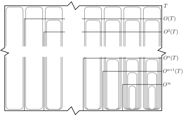
Chapter 1 In the first Chapter we will generalise some of the results from the liter-ature we just mentioned, relatingmutual belief inrationalitywith theiterated elimi-nationof non-optimal strategies. Section 1.1 introduces all of the technical definitions related tostrategic gamesandoptimality operators. Section 1.2 gives a full heuristic treatment of the rest of the Chapter, avoiding as much as possible technical details. We find that to be necessary because there are a number of subtleties involved. Still let us attempt to summarise here what we will do in the technical part of the Chapter. First of all, we generalise the result mentioned above about common belief of rationality to the infinitecase (Theorems 1.1 and 1.2). Then we consider, as did Tan and Werlang [1988] for the finite case,arbitrary stagesalong the way to full common belief. This involves employing a distinction between two different forms of common belief, and borrowing from the literature non-standard‘neighbourhood’ modelsof beliefs in order to distin-guish for example between mutual belief to depthω0and to depthω0+ 1, whereω0 is
the first infinite ordinal. We use the fact that we can make this kind of distinction in neighbourhood models to show that there is a model where for every stage, including the transfinite stages, of iterated elimination of non-optimal strategies, there is some information that ‘rationalises’ it. That is Theorem 1.5, where the model we provide is actually a topologicalneighbourhood model, meaning that the only difference be-tween it and a standard model is that players mightfail to put togetherlargeamounts of information. That is, they might have many pieces of informationϕ1, ϕ2, . . ., and
thereby also have allfiniteimplications of this information, while still failing to draw all the conclusions that might be possible when consideringalltheφn’s.
More generally, neighbourhood models allow for the case where a player does not put her information together, even finitarily. So for example she might believe that ϕ and believe that ϕ → ψ (that ϕentailsψ) and still not believe that ψ. Equivalently: neighbourhood models allow for a situation where a player believes ϕ and believes ψ without believing their conjunction ϕ∧ψ. Thus they are even more ‘permissive’ than topological models, which only allow that players fail to put together infinite amounts of information. Neighbourhood models therefore provide some way to model imperfection of reasoning, where reasoning might be constrained by the nature of the player who for example does not have time to put together her information. In any case, we show that under certain rather weak conditions aboutintrospectivity of beliefs, even this kind of neighbourhood models are enough to prove the kind of result we obtained already for the relational model case. The two different conditions we consider yield two Theorems: 1.3 and 1.4.
Chapter 2 In the next Chapter we introduce formal logical languages, like those used by Hintikka, for reasoning about beliefs. Taking as a starting point arguments from Aumann [1999], we look at a number of reasons for using formal languages in epistemic analysis: for making a distinction between syntax and semantics. One of the arguments that we give in favour of using modal languages in game-theoretic analyses, is that these languages are appropriatelylocal. We catalogue many choices that can be made at the level of the language, usually sticking within the realm of modal languages, though some of them are just notational variants of for example first-order logic. We address the question ofdefinabilityof key notions from game theory, like rationality and common belief. We also spend considerable space on a foundational question concerning the existence of a suitably ‘large’ belief model. That is, we study the property of ‘assumption-completeness’ introduced in [Brandenburger and Keisler, 2006]. This leads us to introduce the ‘type-space models’ used in that work, and to show how they are related to the more standard state-space models. A two-player type-space model is assumption-complete for a language if for every sentence of that language that defines a setB ofb’s types, there is ana type wherea’s information is preciselyB. (Assumption-completeness is related to the ‘comprehension schema’ in set theory.) We examine what assumption-completeness means in state-space models. The principal technical contribution of the Chapter is to prove (Theorem 2.4) that for infinitary modal languagesthere are assumption-complete models.
One of the arguments that we give in favour of using a logical language is that this facilitates reasoning about events across different models, which is very useful in introducingdynamics, in any field but in this case into the study of games. The next two Chapters introduce dynamics into the picture.
Chapter 3 In the first of them, we discuss dynamic epistemic logic, and extend some results to cover the case of neighbourhood models. That Chapter then returns to strate-gic games, and explicitly formalises some interactive reasoning process that are com-patible with the deductive interpretation of game theory. This is one role played by belief dynamics: as a metaphor for the reasoning or computation that is involved in arriving at conclusions about games. We can think of the game as specifying an initial epistemic or informational state, further epistemic states being induced by reasoning from premises saying that the players are rational, reasoning of which we also give a logical account. We interpret this as aprivate but common reasoning process. This attempt to tell a coherent story about the deductive process leads us to look not only at the ‘hard’ information case but also at ‘soft’ information, i.e. to considerrevisable beliefs. We introduce the notion of a ‘rational equilibrium of beliefs’, by which we mean a configuration of beliefs that is stable to further deduction, and we argue that in general using soft information (and so revisable beliefs) is the only way to arrive at a rational equilibrium of beliefs, at least in the case of somenon-monotonicoptimality properties.
Chapter 4 In the last Chapter we turn our attention to applying logical analyses to epistemic aspects of extensive-form games. In an extensive form game players do not, as in the case of strategic games, make their choices entirely independently of the choices made by the other players. That is, an extensive-form game represents a decision process that is extended in time, with players making choices one after the other. The crucial difference in terms of our concerns about beliefs is that the beliefs of the players can change as the game is played. The main contribution we make in that Chapter is to offer an analysis ofbackward inductionin terms of beliefs. In backward induction, players reason about what would happen hypothetically, and in a large class of games (including so-called ‘generic’ games in which no player is indifferent between two different outcomes), this purely deductive reasoning will yield a unique prediction for the game. However, it has been a thorny question exactly what configuration of beliefs or knowledge is required in order to guarantee that players will play according to the backward induction prediction. We offer (Theorem 4.1) such conditions, phrased in terms of dynamics of revisable beliefs, and making crucial use of a notion ofstabilityof belief, and a forward-looking‘dynamic’ rationality.
A similar notion of ‘rational equilibrium of beliefs’ arises in this context, and we use this notion to reason about a simplified version of so-called trembling-hand perfect equilibrium, that we call even-handed, that is a refinement of the usual notion. We suggest that belief revision policies, in concert with lexicographic rationality, are a useful way to think about various solution concepts. Finally, we close the last Chapter by pointing to some limitations of our existing analysis of extensive games in terms of dynamic epistemic logic, specifically that it does not yet give a coherent account of strategic communication.
Origin of the material
This work integrates and builds upon some of my major collaborations over the last three years, when it has been a privilege, as well as very enjoyable, to work with co-authors whom I would like to thank deeply. All errors of presentation and content naturally remain my responsibility.
• Most of the ideas from Chapter 1, and Theorems 1.1 and 1.2, are drawn from [Apt and Zvesper, 2007]. Theorems 1.3, 1.4 and 1.5 build on that collaboration but are original contributions.
• Some parts of Section 2.3 are drawn from [Zvesper and Pacuit, 2010], including Theorem 2.4, which is a generalisation, to the infinitary case, of (op.cit., Theo-rem 2.6).
• Much of Section 4.2, including Theorem 4.1, is drawn from [Baltaget al., 2009]; furthermore, some of the ideas sketched in Section 4.3 are based on work in progress with the authors of that paper.
Believing Rationality in Arbitrary Games
“To infinity, and beyond!” – Buzz Lightyear [Lasseter, 1995]
This Chapter examines mutual belief of rationality in one-shot interaction situations. Like all but parts of the last Chapter of this Thesis, this Chapter is concerned with a purely deductive interpretation, rather than with any element of steady-state inter-pretation, of game theory. So we consider what conclusions players can draw from a relatively minimal amount of information. That information will concern just the (instrumental) rationality of the other players, (where, recall, a player is instrumentally rational just if she acts in her best interest according to her information), and higher-order information about that information.
Thus we look at what it means for players to be rational, and to believe that the other players are rational, to believe that the other players believe that the other players are rational, etc. The most substantial contributions of this Chapter are togeneralisesome standard results from the game-theoretical literature, that connect the different levels of mutual belief in rationality with numbers of rounds of elimination of sub-optimal strategies. That generalisation has three parts to it:
1. As we explain in a moment, our theorems cover a broad class of optimality notions.
2. They also coverinfinitegames, where the results in the literature generally look at finite games.
3. Finally, we consider a larger class of models for beliefs, which means that we make very few assumptions about the ways players put their beliefs together. In terminology that we introduce later in the chapter:
(a) We allow for the case of ‘relational’ belief models in which players need not be ‘positively or negatively introspective’.
(b) We also allow for the more general case of ‘neighbourhood’ belief models, in which players not only lack those introspection properties, but also do not necessarily ‘put their beliefs together’, i.e. believe all the things that follow from their beliefs.
If everybody believes some propositionE, then we say that there ismutual belief ofE’; if everybody believes that everybody believes that E, we say there is second-level mutual belief ofE, and so on. If there is mutual belief ofE on all levels, this is calledcommon belief ofE.1 As we will see, this definition can be made formal in two
ways, depending on whether one includes only allfinitelevels of mutual belief, or ar-bitrarylevels of belief, including levels fortransfinite ordinals. That distinction is not usually made in the game-theoretical literature, and the models for beliefs commonly used there do not allow for the distinction to be made. Aumann [1976] was the first to formalise a notion of common knowledge (or as we might say: common true belief), and in his framework of ‘partition structures’ the distinction cannot be made, nor can it be made in the more general case of ‘relational models’. However, it is possible to make this distinction in other, yet more general, ‘neighbourhood’ and ‘topological’ models for beliefs. We will exploit this distinction when we look at different levels of mutual belief of rationality in infinite games.
Rationality can be defined in many different ways, depending on what notion of ‘optimality’ is used by the players. In turn those different notions of optimality induce operators that reduce the game matrix by eliminating sub-optimal strategies. The first way in which our results are a generalisation of existing ones is that they are phrased not in terms of a specific optimality operator but always in more general terms.
So the results that we will prove all establish, roughly speaking, something of the form:
(?) Rationality plus α-level mutual belief in rationality is equivalent to all players avoiding strategies that are eliminated within 1 + α rounds of elimination of non-optimal strategies.
The second generalisation is that we allow for the possibility that there might be an infinite number of objects of choice for any of the players, i.e. we give results for games witharbitrarystrategy sets. Thus when we writeαabove, we mean it to refer to an arbitrary (possibly infinite) ordinal.2 We will show why this entails, for one
direction of the ‘equivalence’ established by our theorems, considering neighbourhood
1What we call ‘mutual belief’ is sometimes called ‘general belief’ in the literature. Note that,
ac-cording to our terminology, mutual belief is in generalnotthe same thing as common belief.
2Finite ordinals are just natural numbers1,2, . . .. Transfinite ordinals are studied in set theory
[De-vlin, 1993], and their arithmetic is not the same as that for finite ordinals, so that in particular for infinite ordinalsα= 1 +α6=α+ 1. Therefore (as we explain in Section 1.2 below) it is crucial that we write ‘1 +α’ in formulating the various theorems we prove.
and topological models. This in turn means that we will have to define what it means, in neighbourhood models, for a player to berational, i.e. to extend the existing definition from relational models.
One half of the the final generalisation involves showing that in relational (or indeed topological) models, no further ‘introspection’ properties are required of players in order to obtain the result. The other half again involves using neighbourhood models. In those each player might fail to ‘put together’ her pieces of information, or indeed to ‘draw conclusions’ from her information: formally, her information neighbourhoods need not be closed for intersection, and need not be monotonic. Here we present two options in order to get our equivalence. The first is to introduce the new notion of ‘co-mutual’ belief, that we show is enough on neighbourhood models to get (?) with ‘co-mutual belief’ replacing ‘belief’ even if players do not haveanyintrospection properties. The second is to show that with just one minimal introspection property, we can get the result on neighbourhood models.
Background literature
The starting point in game theory for our own small contributions here are [Bernheim, 1984; Pearce, 1984; Tan and Werlang, 1988]. Those papers each show the connection between mutual belief of rationality and the elimination of non-optimal strategies. All of them consider onlyfinitegames, and each focuses on only one type of optimality. The more abstract approach of arbitrary monotonic operators, and the generalisation to infinite games, is studied in [Apt, 2007a].
On the side of interactive epistemology, there was some work on formal episte-mology in the modal logic tradition, started by [Hintikka, 1962]. Aumann brought the attention of game theorists to the notion ofcommon knowledge, by providing an ele-gant formulation of it and theorem about it [Aumann, 1976]. As we have said, it turns out that there are different ways to define common knowledge for infinitary cases; this fact was first established by [Barwise, 1988], and discussed further in [Heifetz, 1999; Benthem and Sarenac, 2004].
Barwise’s ‘situation semantics’ framework was shown in [Lismont, 1994] to be equivalent to using ‘neighbourhood models’, developed in [Scott, 1970], and discussed in the textbook [Chellas, 1980]. A modern logical model-theoretic approach to neigh-bourhood models is presented in [Hansen et al., 2009]. [Heifetz, 1996] also studied common belief on neighbourhood models.
Topological models for modal logic, that we also use below, originate in the work of McKinsey and Tarski [1944], and are studied from a contemporary logical perspective in [Benthem and Bezhanishvili, 2007]. They are used for epistemic logic in [Ben-them and Sarenac, 2004], where again the distinction between two different varieties of common belief is drawn.
Finally let us remark that since players in neighbourhood models do not necessar-ily put their information together, using neighbourhood models to represent players’ beliefs is a partial way to address the problem of ‘logical omniscience’, i.e. the
prob-lem that players believe all logical validities. We do not pursue that connection further here, and so do not entertain either of the two classical ways of addressing logical om-niscience: the use of so-called ‘impossible worlds’ [Hintikka, 1975] or the distinction between implicit knowledge, which is logically omniscient, and explicit knowledge which is not [Faginet al., 1995].
Organisation of the Chapter
In Section 1.1, we spend some time going over standard definitions for game theory, including of strategic games.3 In that Section we do not yet make any novel
contri-butions. We present there the ‘optimality operator’ approach, and we show how the optimality operators can be instantiated by a number of concepts familiar from game theory, including avoiding strategies that are strictly dominated, and so on. Each con-cept can induce a number of different optimality operators depending on some details, including whether we consider pure or mixed strategies, and so on. (We also discuss mixed strategies and the connection, sometimes made in the literature, between them and beliefs.)
Then in Section 1.2 we give, avoiding as much as possible technical details, an ex-planation of the theorems that we will prove in Sections 1.3 and 1.4. In Section 1.3 we introduce formally therelationalmodels of belief, and mention the introspection prop-erties often attributed to players. The theorems in that Section relatecommon belief of rationality to the iterated elimination of non-optimal strategies. So in Section 1.3 we considerfull common belief of rationality, which corresponds to finishing the process of iterated elimination of non-optimal strategies. But the elimination algorithm works in a stage-wise fashion, and we are interested in finding correlates on the epistemic side for each state in the process. In Section 1.4 we therefore look at intermediate (possibly transfinite) stages. As we explain in more detail in the heuristic treatment in Section 1.2 leads us to use neighbourhood models for belief, this means we have to use neighbour-hood models for belief, and we prove the mentioned correspondence betweenα-level mutual belief in rationality with1 +αrounds of elimination of non-optimal strategies. To re-iterate: Section 1.1 mainly repeats material that could be familiar to the reader well-versed in game theory, so such a reader might prefer to skip that Section except for looking briefly at the definition of optimality operator (Definition 1.2) and outcome ordinal (Definition 1.3).
1.1
Strategic games and optimality operators
As a preliminary to the material in this chapter, we will make formal our talk from the Introduction of strategic games and game reduction operations.
3The small games we looked at in the Introduction were all strategic games. Strategic games are also
sometimes called “games in normal form”, for example by von Neumann and Morgenstern [Neumann and Morgenstern, 1944] in their foundational work on game theory, to which the field owes its existence.
Recall that strategic games are intended to represent one-shot simultaneous-choice interactions. So there will be a setN of players, and each playeri ∈ N will have a set of ‘choices’ or ‘strategies’ denotedTi. These will be unanalysed, primitive objects
in the definition of strategic game. The set ofstrategy profilesoroutcomes, denoted T, is then just the Cartesian productQ
i∈NTi: an outcome specifies what strategy each
player chose.
The other ingredient will be the preferences, or ‘utilities’, of the players inN over the outcomes. We will allow strategic games to be defined withordinal preferences or with cardinal preferences. With ordinal preferences, we state that players have a consistent ‘preference order’ over all possible outcomes of the game. This boils down to saying that given two possible outcomes, they can say which one, if either, they prefer, in such a way that we cannot catch them out as preferring a over b, b over cand c over a. That players have consistent ordinal preferences is of course a non-trivial statement, but it is a little less drastic than assuming that players havecardinal preferences, which says that the players assign a particular real number (element of the continuum) to every possible outcome of the game. Cardinal preferences over a set of outcomesT naturally induce ordinal preferences: if the valueiassigns toais greater thani assigns to b theni prefersa over b. But cardinal preferences are strictly more expressive than ordinal preferences: clearly different cardinal preferences can induce the same ordinal preferences. (For example whereT is{a, b}, ifiassigns2toaand3
tobthis is ordinally equivalent toiassigning0toaand300tob.)
Nonetheless, ordinal preferences will be sufficient for almost all of our purposes, and are conceptually a little less questionable than cardinal preferences. Throughout this thesis we will prefer to talk about games with ordinal preferences, though some-times (for example in the present Chapter when we will talk about optimality operators from the literature which involve mixed strategies) we are forced to talk of games with cardinal preferences. Furthermore, sometimes when defining a game it is easier to write down cardinal preferences than ordinal preferences, but they can be thought as simply a shorthand notation for what is really an ordinal preference relation.
Definition 1.1. Fix some set of playersN.
1. Astrategic game with cardinal preferencesforN is a tuple(Ti, πi)i∈N, where
Ti is playeri’s set of ‘choices’, also called her ‘strategies’, and πi : T → Ris
her ‘payoff function’.
2. a strategic game with ordinal preferences (sometimes in this Chapter and the next just called a game), is a tuple (Ti,≥i)i∈N, where each ≥i is a total order
relation overT.4 3. T =Q
i∈NTi is the set ofstrategy profilesoroutcomes.
4I.e. a total transitive antisymmetric relation. We write>ifor the strict version of the relation (s >i
There are two natural ways to define subgames. Firstly, as tuples (Si)i∈N with
Si ⊆Tiof subsets of the strategy sets in the original game; these we will callsubgames
(we do not include the preference information in the definition of a subgame, so a subgame only makes sense as a game in the context of the original game of which it is a subgame). The second way would be to define them as subsetsS ⊆T of the strategy profiles in the original game; these we will call restrictions. Any subgame (Si)i∈N
defines a restriction: Q
i∈NSi. Conversely, it is only ‘rectangular’ subsets S ⊆ T
(restrictions) that are definable in this way. For example if the original strategies were
({U, D},{L, R}), then the restrictionS ={(U, L),(D, R)}clearly is not definable by any subgame. Although in this Chapter we will mainly be interested only in rectangular restrictions, still we often use restrictions just because they are sometimes notationally easier.
We need to introduce a few useful pieces of standard notation for manipulating strategies and restrictions. For any playeri, we writeT−i to meanQj∈N−{i}Tj. And
given any si ∈ Ti and s−i ∈ T−i, by (si, s−i) we mean the relevant element in T.
Similarly, givenSi ⊆ Ti andS−i ⊆ T−i, the expressionSi×S−i denotes the relevant
subset ofT. Given a restriction S, for any playeri, we write Si to mean the set ofi’s
strategies occurring in some profile inS:
Si ={si ∈Ti | ∃s−i ∈T−i : (si, s−i)∈S},
and also extend this notation toS−iin the analogous way. Sometimes we will refer
in-terchangeably to a rectangular restriction and its corresponding subgame, so we could write for example (when the set N of players is irrelevant or clear from the context)
(T,≥)to refer to the game(Ti,≥i)i∈N.
Let us adapt a motivating example from [Morgenstern, 1928] (actually we entirely change the story, but the message is similar). Suppose Sherlock Holmes and his neme-sis Moriarty are on a train from London which will stop only at Canterbury and Dover. The latter has a gun and hopes therefore to catch the former, and so wants to alight at the same stop as him. Holmes on the other hand, who has no way to defend himself save his cunning, wishes to evade capture, and so wants to alight at a different stop. Apart from that, Holmes would prefer not to stay on the train very long, because if he evades Moriarty he would like to return to London that evening. Moriarty on the other hand hopes to escape to France, so staying on this train to Dover is his preferred option. We can describe the game as follows:
N ={h, m}
Th =Tm ={D, C}
(C, D)>h (D, C)>h (C, C)∼h (D, D)
(D, D)>m (C, C)>m (C, D)>m (D, C)
Here the players are h (Holmes) and m (Moriarty), the strategies for either are D andC (Dover or Canterbury), and so the outcomes are e.g.(C, C)they both alight in Canterbury, or(C, D)Holmes alights at Canterbury, evading Moriarty who remains on
the train until Dover. The preferences are faithful to the story, so that for example for Moriarty the best option is for both Holmes and he to alight at Dover so that the evil mastermind can shoot the detective and hop aboard a ferry to the Continent.
We could also denote the situation as a game with cardinal preferences as in Fig-ure 1.1, where Holmes is the row player (choosing the row), and Moriarty the column player. What option will the players choose? Actually neither option for either player
C D
C 0,2 2,1
D 1,0 0,3
Figure 1.1: The game Holmes and Moriarty are playing.
would be ruled out by any of the ‘optimality’ operators we consider later; intuitively this is because none of the options are obviously irrational. Indeed this is an example where a one-shot analysis of the situation does not have much to say. Holmes’ fa-mously flawless and yet insightful logic should reveal to him what is the best solution in his dilemma: alight at Canterbury or stay on until Dover. Let us imagine a dialogue between Holmes and Watson5.
Watson: Moriarty wants to go to Dover, therefore you should alight at Canterbury, and live to capture that swine on a later date.
Holmes: How simple-minded you are sometimes Watson. Apparently you have forgotten with whom we are dealing. Do you really think that Moriarty is not able to put himself in my shoes, and to reason in precisely that way?
W:Oh yes I see Holmes, so you mean you should alight at Dover, because Moriarty knows that you know that he wants to go there, and so will expect you to alight at Canterbury, and so will alight there to try to catch you. How clever you are, to out-think him that way.
H:Again Watson you are not thinking enough. Moriarty will be able to perform that reasoning as well. . .
W:So you mean I was correct before, but for the wrong reasons: alight at Canterbury, also that way you can be back in time for tea!
H:(Sighs) I fear you are not getting my point.
What is Holmes’ point? The fact is that if there were some deductive reasoning that could lead Holmes to see that C (or D) was the best option, then since Holmes’ op-ponent is also highly intelligent, Moriarty could also follow that reasoning, thereby alighting atC (respectivelyD), and shooting Holmes. In which case clearly Holmes’ reasoning did not in fact lead him to the best option.
5We mercilessly misrepresent the characters of Holmes and Watson to fit stereotype rather than their
actual nature in the books by Conan Doyle. Also, for the sake of our story, recall that the cunning detective’s trusty side-kick is not present.
Therefore since Holmes cannot make a decision based purely on deduction, he is forced to throw reason to the wind and alight wherever his intuition tells him to. I.e., he cannot actually make the decision, but,if we assume that Moriarty would be capable of re-creating Holmes’ reasoning, the best option for Holmes appears to be that he must randomise between the two options.
That is, Holmes should play a so-calledmixed strategy. In the case of games with ordinal preferences, mixed strategies would simply besets of strategies; in this case since there are only two options,{D, C} is Holmes’ mixed strategy. Mixed strategy profiles, that specify a mixed strategy for each playeri ∈ N, are in this case just sub-gamesof the original game. There would be several different ways to lift the existing preference relation over pure strategy profiles to a relation over mixed strategy pro-files. It is not clear what grounds to use to choose among the different liftings, but we do not pursue this matter further, since mixed strategies are generally only consid-ered in the case of cardinal preferences, where a much more fine-grained distinction between mixed strategies is available. Indeed the literature generally only considers mixed strategies in terms of cardinal utility (see for example [Osborne and Rubinstein, 1994, Chapter 3]), so we will take ‘mixed strategy’ to imply that the underlying game is one of cardinal utility.
For games with cardinal preferences, mixed strategies are more complicated enti-ties: in these games, a mixed strategy for playeriis aprobability distribution overTi.
(A probability distribution overTi, forfiniteTi, is a functionσ : Ti →[0,1]such that
P
si∈Tiσ(si) = 1.) There is a debate in the literature of game theory as to how to
inter-pret mixed strategies. We favour taking them simply to mean that the player literally randomises over his choices with the relevant probabilities, but this only colours the way we talk about them, and not the content of any theorems we prove that relate to them.
Another common interpretation has it that mixed strategies really represent abelief by the opponents about how a player will play. This is argued for in for example [Aumann and Brandenburger, 1995]. While we recognise that one can represent some elements of a player’s beliefs as a mixed strategy, still to say that the mixed strategy that a player actually players is a belief by the opponents is a superficial treatment of the notion of belief. If a playeri plays a mixed strategyσ, it would mean that all of the players have thesame belief regarding i’s behaviour. More importantly, such a simplistic approach means that any kind of higher-order belief (i’s belief about j’s belief) collapses. This, as we indicate in Chapter 4, might well make sense in an equilibrium where all beliefs become common belief. So it arguably fits with some steady-state interpretation of game theory (and it is indeed Nash equilibrium, and so a steady-state interpretation, that is considered in [Aumann and Brandenburger, 1995]). However, clearly it does not suit thedeductiveapproach that should be applied to truly one-shot interaction situations.
To repeat: in the deductive approach, playing a mixed strategy should really mean randomising, with the allotted probabilities, between the different options, and does not represent a belief or ‘conjecture’ by the other players about what the one player will
do. We do not want always to assume that the players have this option to randomise. Indeed, if this option is available to the players then we might want to say that really they are in a bigger game, the so-called ‘mixed extension’ of the original game, in which the strategies are the mixed strategies from the original, and the payoffs are given by what is called the “expected utility” function.
For finite Si, we write ∆Si to mean the set of probability distributions over Si.
Then in a game with cardinal preferences the set of mixed strategies of playeriis∆Ti,
Generally we will useσ to refer to mixed strategy profiles (yielding a mixed strategy σi ∈ ∆Ti for each player i). The canonical way to extend a utility function over
pure strategy profiles to a utility function over mixed strategy profiles, that defines the preferences in the mixed extension, uses the notion of “expected utility” (that might better just be called “mixed utility”):
µi(σ) =
X
s∈T
σ(s)·πi(s).
Note that we cannot without some other stipulation extend this definition to the case whereT is infinite. That is because examples can be constructed in which the expected utility of a given strategy profile would be infinite. So we will assume in general, when we talk about expected utility and mixed strategies, that there are a finite set of strate-gies. (Another solution is to consider only probability distributions withfinite support, i.e. in which only a finite number of strategies are assigned non-zero probability, or to place some restriction that excludes ‘badly-behaved’ utility functions, but we do not need to go into any further detail here.)
Pure strategies are in effect simply ‘degenerate’ cases of mixed strategies, in which all of the probability mass is assigned to a single element, and sometimes we will write a termsi denoting a pure strategy to mean the corresponding mixed strategy that
associates probability1tosi, and0to all other ofi’s pure strategies. (So in set-theoretic
notation it would be the function{(si,1)} ∪((Ti− {si})× {0})).
The next concept we need to formalise in this Section is that of game reduction operators, or ‘optimality operators’. An optimality operator for playeriis supposed to say which strategiesishould ‘throw out’ on the grounds that they are sub-optimal. We want our approach to be as generic as possible, and so while many specific optimality operators exist, the results we will present in this Chapter will hold for optimality operators that satisfy a certain condition of monotonicity. An individual optimality operator6for playeritakes a game and a restriction and returns a set of strategies. Definition 1.2. Anindividual optimality operatorsfor playeriis any (class-)function that, given a gameG= (Tj,≥j)j∈N withi∈ N and a restrictionS ⊆T, returns a set
Si0 ⊆Ti ofi’s strategies.
6We sometimes omit the word ‘individual’, which is there to distinguish it from ‘collective’
Often it will be convenient to fix a gameGand to consider optimality operators as functionsOiG : 2T → 2Ti. (And sometimes whenGis clear from the context we will
drop the superscriptG.)
This definition is of course a little too abstract to really capture any notion of opti-mality. In actual examples optimality operators will be defined in terms of the players’ preferences, and will capture the notion that optimal choices are in some sense pre-ferred over sub-optimal choices. We will give examples of such optimality operators later in this Section, but first let us give two important properties of optimality opera-tors that we will consider:
An operatorO iscontractingif for all restrictionsS, O(S)⊆ S. AndO is mono-tonicif for all restrictionsSandS0, ifS ⊆S0 thenOi(S)⊆Oi(S0).
The idea behind the argument given to the individual optimality operator for a par-ticular game is that it is intended to represent the restriction of the game that the player thinks she is actually playing in. This will become more formal when we introduce belief models in Section 1.3 to capture the idea of a player ‘thinking’ (or rather, ‘be-lieving’) something. For now the operators remain purely algorithmic, or procedural. We will be interested in combining them and in iterating the resulting operator, that we will call acollective optimality operator, or sometimes (again) just an ‘optimality operator’. So given a family of individual optimality operators(Oi)i∈N, letO denote
the operator from restrictions to restrictions, i.e.O: 2T →2T, defined as follows:
O(S) = Y
i∈N
Oi(S).
Clearly if eachOi is contracting or monotonic then O is contracting or, respectively,
monotonic with respect to the component-wise subset ordering.
Optimality operators actually operate only on rectangular restrictions, and collec-tive operators return rectangular restrictions. So we could have defined them in terms of subgames, as for example in [Apt, 2007c]. We prefer the more general formulation in terms of restrictions simply because it fits better with the rest of our notation.
Fixing some gameG, we will be interested in iterations of this collective operator, starting with the largest restriction, that corresponds to the initial game. LetON denote the class of all ordinals; then given some gameG= (T,≥)and an optimality operator Oforα ∈ ON,Oαis the operation corresponding toαapplications ofO. Precisely, it is defined as follows, where (and this is a convention we maintain throughout)βis an arbitrary ordinal andλa limit ordinal:
O0(T) =T
Oβ+1(T) = O(Oβ(T))
Oλ(T) =T
β<λO β(T)
To make the notation more elegant, we often, when it is clear from the context whatT in question, write simplyOαforOα(T).
A restriction S is a fixpoint of O if O(S) = S. Assume fixed some game G = (T, <). Then for α ∈ ON with Oα(T) a fixpoint, we call that (obviously unique) Oα(T)theoutcomeofOonG, and denote it byO∞
G.7
Definition 1.3. IfG= (T, <), then we call the least ordinalαsuch thatOα(T) = O∞
G
theO-outcome ordinalofG, and write itαO G.
For each ordinal αand optimality operator O, the result of iteratingO α times is a ‘solution concept’, to use the terminology of game theory. The most commonly-considered such solution concept, for a given optimality operator, is its outcome. In Section 1.3 we will be interested in the outcomes of (collective) optimality operators, and will make appeal to Fact 1.1.2.
Fact 1.1. We are guaranteed that, for any gameG:
1. IfO is contracting then it has an outcome (becauseT is a set).
2. IfO is monotonic then it has an outcome, which is the largest fixpointS {S ⊆ T |S ⊆O(S)}(immediate corollary of [Tarski, 1955, Theorem 1]).
Note that while if an operator is contracting it need not be monotonic, or vice-versa, still theoutcomeof a monotonic operator and its ‘contracting version’ coincide, in the sense that given some monotonic operatorO, and definingO(S) = S ∩O(S)as its contracting version, we have the following Fact (cf. [Apt, 2007b, Note 1]).
Fact 1.2. For anyα∈ ON,Oα =Oα.
We can now look at some particular instances of optimality operators from the game-theoretical literature, where each different optimality notion has several different specific instantiations.
The first group of operators that we will look at are those induced by the elimination of strictly dominated strategies. A strategysi isstrictly dominatedby a strategy s0i in
the context ofS−i if
∀s−i ∈S−i, (s0i, s−i)>i (si, s−i).
(For cardinal utility and mixed strategies, simply replace, here and in the rest of the Chapter,(s0i, s−i) >i (si, s−i)byµi(s0i, s−i) > µi(si, s−i).) We writensdi(si, s0i, S−i)
to mean that si is not strictly dominated by s0i in the context of S−i. Now there are
several ways in which we can use this property to induce an operator, which will all have the following form, with different instantiations forAandB:
OiG(S) = {si ∈A| ∀s0i ∈B, nsdi(si, s0i, S−i)}.
7We thus use the same word ‘outcome’ for both the outcomes of a game and the outcome of the
iterated elimination of non-optimal strategies. We do not anticipate that this will cause any confusion, but note of course that the outcome of iterated elimination will in general not yield asingleoutcome in the other sense.
Now there appear to be eight different versions of this operator given by instantiating A with either Si or Ti, and B with one of Si, Ti, ∆Si or ∆Ti (where, as we assume
throughout,G = (Ti,≥i)i∈N, or(Ti, πi)i∈N if it is a game with cardinal preferences).
Some of these operators coincide, but let us use them to introduce our terminology, that we will use for all of the different optimality notions.
IfAis instantiated withSi, we call the operator thecontractingform (since clearly
then it will be contracting), and ifAis instead instantiated withTi we call it the
non-contracting form (even if it might in fact happen to be non-contracting). WhenB is either Si or∆Si then we call the resulting operator the localform, and otherwise we call it
theglobal form. The idea behind the local form will be that player looks only at the possibilities given by her information about the game in order to determine whether there is a better strategy to play, and in the global version does not ‘forget’ possibilities that might be better. The distinction between global and local (and contracting and non-contracting) optimality operators is due to [Apt, 2007b; 2007c]. The last piece of terminology is not surprising: ifB is either∆Si or∆Ti then we talk about themixed
form, otherwise we talk about thepureform (or just drop the qualifier altogether). The observation that the contracting form is contracting is obvious, and indeed clearly holds no matter what property we would put fornsdi. That theglobalform is
monotonicis only a little less obvious, but essentially just uses the fact that it can be defined by a formula which is positive in the argument the operator takes.
Our main interest in this Chapter will be in theglobalforms of the operators, be-cause in general only the global forms are monotonic. Here and in what follows, by Fact 1.2, as long as we are only interested in iterations of a monotonic operator from the initial game, then it does not matter whether we consider the contracting or non-contracting forms.
Furthermore, since we are considering only these iterations starting from the initial game, then notice that onfinitegames (i.e. in which each player’s strategy setTi is
fi-nite), there are actually only two operators. That is established by [Apt, 2007c, Lemma 2], which implies that on finite games the local and global forms of each of the con-sidered operators coincide. Therefore the only distinction that remains is between the mixed forms. A standard example (cf. [Osborne and Rubinstein, 1994, Figure 61.1]) shows the pure and mixed forms do not coincide; see the game illustrated in Figure 1.2. (We read this as a game with cardinal utilities, because there is no way to make
L M R
U 1,3 1,0 0,1
D 0,0 0,3 3,1
Figure 1.2: A finite game distinguishing pure and mixed strict dominance. the distinction with ordinal mixed strategies) In that game,Rfor the column player,b, is not strictly dominated in the context of{U, D}by either of thepurestrategiesLor
M, butisstrictly dominated in the context of{U, D}by for example the mixed strat-egyσb withσb(L) = σb(M) = 0.5, since then for any of the row player a’s strategies
sa ∈ {U, D}, we haveµb(σb, sa)> µb(sb, sa).
Notice that this example illustrates that neither player actually has to end up play-ing a mixed strategy for the possibility that they could play a mixed strategy to af-fect the outcome. Specifically, if we remove R (because it is strictly dominated by {(L,0.5),(M,0.5)}), thenDbecomes sub-optimal for the row player, since the oppo-nent is going to play in{L, M}, so we can removeD, and then go on to remove M, since in the context of{U}it is the only undominated strategy for the column player. So then in the outcome, neither player has a choice left, so they play Land U, both pure strategies. However, the outcome of eliminating strategies dominated by apure strategy is the entire game, since no strategy is dominated.
Conditions for the iterated elimination of strictly dominated strategies on finite games, in terms of the beliefs (actually they also considered knowledge) were first given in [Tan and Werlang, 1988], and their result is one that we will generalise below. The notion of weak dominance is a refinement of strict dominance: a strategy si
can be weakly dominated bys0iin the context ofS−ieven if for somes−i ∈S−i,s0idoes
not do strictly better againstsi,as long as it never does worse. The formal definition,
or rather the schema that defines the same forms as in the case of strict dominance, is as follows:si isweakly dominatedbys0iw.r.tS−i, denotedwdi(si, s0i, S−i), if:
∀s−i ∈S−i,(s0i, s−i)≥i (si, s−i)
and ∃s−i ∈S−i,(s0i, s−i)>i (si, s−i).
Now, although weak dominance has prima facie intuitive appeal, it turns out to be a rather less mathematically well-behaved notion than strict dominance. The first point to notice, that disqualifies it from the scope of the theorems we will prove in this Chapter, is thatneither its local nor global forms are monotonic. For instance in the game depicted in Figure 1.3,Dis not weakly dominated in the context of{L}, yet in the context of the larger set{L, R}, itis weakly dominated. It is precisely examples
L R
U 0,0 1,0
D 0,1 0,0
Figure 1.3: A game illustrating the non-monotonicity of weak dominance. like this that are ruled out by the monotonicity of an operator, so such examples do not exist for strict dominance.
In this example, the outcome is({U},{L}). Notice though that intuitively speaking it is not clear why the players would play these choices, given that together they yield a least preferred option (for both players). In terms of beliefs, the justification should be that although e.g. the row player believes the column player will play L, still she
should leave open the possibility that he will playR. That is not something that the epistemic framework of this Chapter can deal with in general, and it is a topic that we will return to in the next Chapter, when we look at counterfactual beliefs.
Although we will not consider this next issue in any detail, notice also that there would be different ways of putting together an operator for weak dominance that would yield different results. What we mean is that although we have defined collective optimality operators as the intersection of individual optimality operators, there are other possible ways of doing this. Taking an intersection effectively means applying the individual operators simultaneously, whereas we might want instead toiteratethe individual operators. Then in our example, we might apply first the operator for the row player, thus obtaining (sinceDis weakly dominated byUin the context of{L, R}) the restriction({U},{L, R}), andonly thenapply the operator for the column player, which in this case will leave both strategies, so that the outcome of such an operator will be ({U},{L, R}), which is clearly a different outcome from the simultaneous version.
One could even combine the individual optimality operators in more ways, by only partiallyapplying the individual operators. So, to take an example directly from [Os-borne and Rubinstein, 1994, Figure 63.1], in the game depicted in Figure 1.4,M and R are both weakly dominated byL. If we first remove R, U becomes weakly domi-nated leaving the outcome ({D},{L, M}), but if we instead first removeM, thenD is dominated, leaving the disjoint outcome({U},{L, R}). Such a situation can never arise in the case of the monotonic operators.
L M R
U 1,1 0,0 1,1
D 1,2 1,2 0,0
Figure 1.4: A game illustrating the order-dependence of individual weak dominance operators.
The final kind of optimality we consider is a different strengthening of strict domi-nance: best response. The idea here is that a strategy is only optimal if it can be justified (‘rationalised’, to borrow the terminology of Bernheim [1984] or Pearce [1984]) by a belief that the other players will play in such-and-such a way. Believing that play-ers will play in such-and-such a way could mean two things: thinking that they will play according to a given pure strategy; or thinking they will play according to a given mixed strategy.
In the former case, we say thatsiis apoint best responsein the context ofS−iand
amongB (where as aboveB ∈ {Si, Ti}determines whether it is the local/global and
pure/mixed form of the property), writtenpbr(si, B, S−i), just when