Poverty, Inequality and Growth in Zambia during the 1990s

Session Number:

6A

Session Title:

Measures of Poverty and Social Exclusion

Paper Number:

6

Session Organiser:

Stephen Jenkins

Discussant:

Patricia Ruggles

Paper Prepared for the 26

General Conference of

The International Association for Research in Income and Wealth

Cracow, Poland, 27 August to 2 September 2000

POVERTY, INEQUALITY AND GROWTH IN ZAMBIA DURING THE 1990S

Neil McCulloch, Bob Baulch

and

Milasoa Cherel-Robson

For additional information please contact:

Neil McCulloch

Institute of Development Studies

University of Sussex

Brighton

BN1 9RE

UK

[email protected]

Fax: (+44) 1273 621202/691647

Telephone: (+44) 1273 877223

This paper is placed on the following websites:

www.stat.gov.pl

www.econ.nyu.edu/dept/iariw

www.ids.ac.uk

Poverty, Inequality and Growth in Zambia during the 1990s

Neil McCulloch, Bob Baulch

and

Milasoa Cherel-Robson

Institute of Development Studies

University of Sussex

Brighton BN1 9RE

UK

16 June 2000

Introduction

Most people in Zambia are poor. Evidence from household surveys and poverty assessments conducted during the 1990s show that between 70 and 80 per cent of the population spend less than the national poverty line (Republic of Zambia 1997a). Zambia is also a very unequal society – the Gini coefficient in 1996 was 0.52, a high value by international standards. This reflects a society in which the top 10 per cent of the population receive over half of the per capita income, whilst the bottom 10 per cent receive 0.5 per cent (Republic of Zambia 1997a).

Since the election of the Movement for Multi-party Democracy (MMD) government in 1991, the Zambian authorities have implemented widescale economic reforms. In addition to undertaking a sharp stabilisation programme early in the decade, the government have implemented reforms in agricultural marketing, a large privatisation programme, sweeping trade policy reforms and, more recently, public sector reform. The implementation of stabilisation and structural reforms in any country can have a major impact upon poverty and inequality. In order to obtain an accurate view of these effects, it is necessary to have nationally representative household survey data from both before and after the reform episode.

Fortunately, there were four such surveys in Zambia during the 1990s – the first in 1991 coincided with the election of the new government, and further surveys were conducted in 1993, 1996 and 1998. This paper reanalyses the household survey data from three of these surveys in order to chart the evolution of poverty and inequality during the 1990s. In addition, the economic policies pursued during the 1990s are described in detail, enabling linkages to be drawn between the policies implemented and the observed changes in poverty and inequality.

The next section briefly describes Zambia’s economic performance since independence. This is followed by a detailed description of economic performance during the 1990s and the economic policies pursued, focussing upon stabilisation, agricultural marketing reform, trade reform and privatisation. We then describe the household survey data which we use and the steps taken to ensure the comparability of different surveys across time. The calculated changes in poverty and inequality are then presented. In

1 _{The paper has been produced as part of a series of studies on Poverty Dynamics in Africa supported by the World}

Bank. The authors would like to thank Lionel Demery for his excellent technical management, the Zambian CSO for access to the data and Miss Efrida Chulu and Mr. Solomon Tembo for clarification of the survey methods, and Howard White for numerous valuable comments and suggestions. Jenny Edwards provided excellent secretarial support. All errors remain the responsibility of the authors.

addition poverty-growth and poverty-inequality elasticities are calculated, to assess the potential

contribution of growth and changes in inequality for future poverty reduction and the growth rate required to achieve the International Development Target of halving the proportion of people in poverty by 2015 is calculated. We conclude with a discussion of how economic policy may have contributed to the changes in poverty and inequality observed.

Economic Performance 1964-1991

At independence in 1964 Zambia was one of the most prosperous countries in sub-Saharan Africa. With substantial agricultural and mineral natural resources the prospects for growth and human development seemed bright. However, poverty was extremely high and the new government faced a major challenge to redress the large inequalities which existed in the distribution of income.3 Initially Zambia followed fairly liberal political and economic policies with policies focussed on the provision of infrastructure and services for the bulk of the population. However, the Mulungushi Declaration in 1968 and its implementation in 1972 marked a change towards a more restrictive policy environment with a heavy role for the state in national development. These policies included a much more inward looking approach to development with manufacturing protected by high tariffs whilst an overvalued exchange rate encouraged inefficient capital-intensive development for the domestic market. Price controls for major commodities were introduced and credit was directed by the National Commercial Bank. In addition the government directly took control over many parts of the manufacturing sector, agricultural marketing and the mining sector.

During the first ten years after independence rising copper prices and high levels of investment resulted in economic growth averaging 2.4 per cent a year. However, this was still below the rate of population growth resulting in falling per capita incomes. Although rural and urban inequality were individually lower than national inequality (with Gini coefficients of 0.48 each in 1974-75), the large gap between average urban and rural incomes resulted in an overall Gini of 0.59 in 1974 suggesting that inequality increased during the first ten years.

After 1975 Zambia faced a collapsing copper price, conflict in neighbouring countries and the severe repercussions of the first oil shock. Initially the collapse in the copper price was seen by the government (and the international community) as temporary. The government therefore borrowed to maintain levels of consumption. However, by the early 1980s it was apparent that the somewhat half hearted attempts at reform during the 1970s had not been effective. A more serious IMF/World Bank Structural Adjustment Program (SAP) was attempted between 1983-85 with strong conditions attached. The government abandoned this agreement and re-imposed numerous controls in May 1987 after political discontent resulted in food riots in the Copperbelt at the end of 1986.

However, as the economy continued to decline the government had little option but to enter into fresh negotiations with the IMF. In June 1989 it decontrolled all consumer goods prices except maize and in early 1990 the government and the IMF drew up a new Policy Framework Paper outlining the economic policies to be pursued between 1990 and 1993. As part of this framework, the government increased the prices of high grade maize meal by over 100 percent in June 1990. This led to widespread rioting in Lusaka and the major Copperbelt towns (Simutanyi 1996). Normal relations with the World Bank were resumed in March 1991 and the IMF’s Rights Accumulation Programme commenced the following month effectively enabling Zambia to reschedule its debts to the IMF.4 However, the government’s agreement to hold elections in 1991 undermined its commitment to implement painful reforms and in June 1991 it requested the IMF to postpone a scheduled round of reduction of maize meal subsidies. The IMF refused and suspended all financial disbursements to Zambia. Inflation rose sharply as the government printed money to fund civil service pay increases and to fund the election campaign (Simutanyi 1996).

2

This section draws heavily on (World Bank 1994a).

3

Data for 1959 show an overall Gini coefficient of 0.48. Figures for 1964 are not available.

4

Trends in Economic Indicators during the 1990s

By the early 1990s real consumption per person had fallen by two-thirds over 15 years. More worrying still was the decline in certain social indicators. Zambia’s performance in the 1960s and 1970s on social indicators such as school enrollment, infant and under-5 mortality and the number of malnourished children was good. However, continued economic decline saw improvements falter. Gross enrollment rates in primary schools showed a downturn after 1985; infant mortality which had fallen from 147 in 1969 to 79 per 1000 live births in 1977-78, actually rose to 107 during 1987-91; a higher percentage of children under 5 years of age were stunted or wasted in 1990/91 than in 1970/71. Against this background, there were strong hopes for economic recovery and growth in the 1990s.

However, Zambian economic performance in the 1990s has been disappointing. Both 1990 and 1991 saw declines in GDP driven by substantial declines in the mining and quarrying sector. A severe drought in 1992 resulted in a collapse of agricultural value-added by one third, although increases in mining and manufacturing output resulted in an overall GDP growth of 2.1 percent. Further declines in mining and manufacturing output in 1993, 1994 and 1995 resulted in negative GDP growth in each of those years; mining and quarrying output and manufacturing production both declined by almost one third between 1992 and 1996. Similarly, construction value-added fell in every year from 1990 to 1996 and value-added in the wholesale and retail trade fell in five of the six years between 1990 and 1995. In 1996 there was a slight recovery in mining and manufacturing complemented by substantial growth in wholesale and retail activities and real estate and business services. This resulted in an overall GDP growth of 6.6 percent in 1996 and 3.3 percent in 1997 (which was principally caused by an increase of one third in construction activities). These are the only two years in the 1990s registering positive per capita growth. Estimated figures for 1998 show a return to negative GDP growth of around 2 percent. Figure 1 shows GDP and GDP growth over the 1990s. (International Monetary Fund 1999).

Performance on inflation over the decade has been slightly better than that on growth. The decade started with high inflation accelerating to a peak of almost 200 percent in 1993 due to excessive monetary expansion. However, the introduction of high real interest rates on Treasury bills along with the implementation of cash budgeting brought inflation down to 55 percent in 1994 and subsequent tight monetary policy reduced inflation to around 25 percent in 1998.5 Interest rates mirrored the performance of inflation, with low nominal (and negative real) interest rates in the early 1990s replaced suddenly by high nominal (and positive real) interest rates in mid-1993. As inflation fell from 1994 onwards, so did interest rates but moderate positive real interest rates prevailed in most years.6 The evolution of the real exchange rate was influenced by the movements in interest rates. The 1992 budget presented a policy of rapid depreciation (Andersson 1995) which, when combined with negative real interest rates resulted in continued depreciation of the Real Effective Exchange Rate (REER). However, the introduction of positive real interest rates in mid-1993 resulted in a switch back to Kwacha and the maintenance of relative tight monetary policy since then has resulted in a steady appreciation of the REER.

Export performance in the 1990s has also been mixed. Total exports (f.o.b.) fell by over 30 percent between 1990 and 1998. This reduction was caused principally by a collapse of metal exports by almost half over this period. Copper, which has always been Zambia’s largest and most important export, collapsed in value from over US$ 1 billion in 1990 to US$ 430 million in 1998. The volume of copper exports fell by 42 percent in the face of a continuing downward trend in copper prices – prices in 1998 were more than 30 percent below those at the start of the decade.7 By contrast cobalt prices more than trebled between 1990 and 1997, doubling the value of cobalt exports between 1990 and 1998. Also,

5

The sequencing and timing of the stabilisation measures and the continuation of the cash budget have been heavily criticised. (White 1998) discusses several different perspectives on the design and implementation of reforms in the 1990s.

6 _{The exception was 1997 where retirement of government debt to the Bank of Zambia resulted in much lower nominal}

interest rates and therefore negative real rates.

7

For an in depth analysis of the Zambia’s management of copper price shocks in the earlier period between 1964 and 1980 see (Aron 1999).

encouragingly, the value of non-metal exports has more than trebled since 1991. Thus the decline of some heavy industrial activities appears to be complemented by growth of more competitive exports better reflecting Zambia’s comparative advantage (International Monetary Fund 1999).

Employment data for the 1990s are only readily available for formal sector activities. Zambia’s labour force is estimated to have grown from around 3.2 million in 1991 to over 4.7 million in 1998. The formal sector only employed 17 percent of the labour force in 1991 and, despite the 46 percent increase in the labour force, formal sector employment has declined by 15 percent now constituting less than 10 percent of employment. Most of this decline has resulted from major restructuring in the mining and manufacturing sectors which commenced in 1992. Mining and quarrying employed 64,800 workers in 1991 – by 1998 employment had fallen to 39,434. Formal manufacturing has also suffered severe decline with employment falling over 40 percent from 75,400 in 1991 to 43,320 in 1998 (Republic of Zambia 1994a; Republic of Zambia 1999). Employment in construction collapsed between 1990 and 1995 to less than one third of its 1990 level, but has since seen strong growth. Similarly employment in transport and communications and in distribution and trade saw small reductions between 1992 and 1995, but have been growing since the mid-1990s. Despite the introduction of a Public Sector Reform Programme, employment in public administration remained relatively stable until 1996 but has reduced slightly since (Seshamani and Kaunga 1999).

Figure 2 shows formal sector employment for central government, local government, parastatals and the private sector. It is clear that the reduction in formal sector employment has come predominantly from job losses in the parastatal sector rather than substantial reductions in public sector employment. Until 1996 job losses in the parastatal sector were not compensated by corresponding increases in private sector employment. However, as the privatisation programme gathered momentum in 1996 and 1997 private sector employment increased, although much of this increase may be due to a reclassification of workers formally in the parastatal sector. Total formal sector employment continued to decline.

Declining employment in the formal sector displaced a large number of workers into the informal sector. Data on informal sector employment is poor. The CSO estimate that total informal sector employment was around 2.3 million in 1993 of whom around 59 percent were self-employed or owner-operators, whilst the others were employed in small enterprises or were unpaid family workers (Republic of Zambia 1997b). Informal sector employment has grown substantially in recent years with a 35 percent increase in informal agricultural employment and a 15 percent increase in informal non-agricultural employment between 1995 and 1998 (Republic of Zambia 1999). However, since the definition of informal sector employment includes unpaid work it is not clear the extent to which this increase reflects a genuine increase in opportunities rather than a reclassification of workers displaced from formal sector activities.

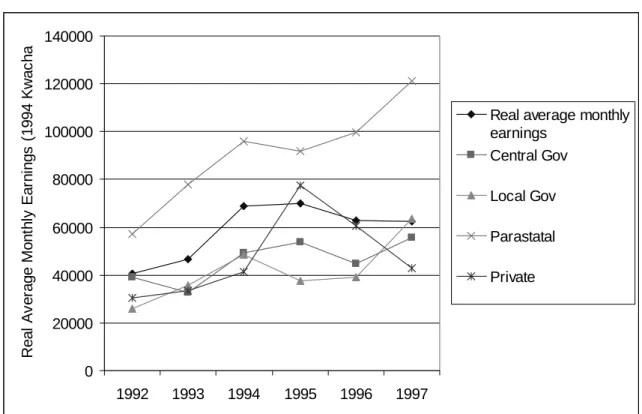
Has the reduction in formal sector employment resulted in higher wages for those remaining? Figure 3 shows average real monthly earnings between 1992 and 1997 for Central and Local government, parastatals and private sector employees. Average monthly real earnings in the formal sector rose steadily from 1992 until 1995. The large rise in real earnings between 1993 and 1994 resulted from the sudden reduction in inflation between those years. However, real earnings declined by over 10 percent between 1995 and 1996 as real earnings fell in both central government and the private sector. The data suggest that the increase in overall real average earnings is driven by the high and rising real earnings in the parastatal sector which have more than doubled in real terms over the period. Real earnings in local government have also increased by 143 percent between 1992 and 1997, whilst central government earnings have risen by 43 percent and private sector earnings by 42 percent. Unlike the parastatals and local government, private sector earnings have sharply declined since 1995. However, we interpret these figures with some caution since some of changes may be due to a change in the classification of workers from the parastatal sector to the private sector.

Economic Policy Reform since 1991

We now turn to consider economic policy reform since 1991. By 1991 reform had become politically and economically unavoidable. In October of that year the Movement for Multi-Party Democracy (MMD) government was elected on a platform of major reforms designed to release the economy from controls and facilitate market-based growth. Since then the Zambian authorities have undertaken numerous steps to liberalise markets and initiate reform. These include exchange rate liberalisation, tax reform and

expenditure restructuring, the removal of many subsidies including the maize meal and fertiliser subsidies, the decontrol of agricultural prices, the privatisation of agricultural marketing and the introduction of user fees in health and education (White 1997).

The major reforms implemented are explored in some detail below since they help to explain both Zambia’s macroeconomic performance and the trends in poverty and inequality described in the following sections. The MMD government implemented major reforms in four areas: stabilisation; agricultural maize marketing; trade and industrial policy; and privatisation. We explore each in turn below.

Macroeconomic Stabilisation

When the MMD government took power the economy faced numerous problems. GDP was around two-thirds of the level of the late 1960s after two decades of erratic and often unsuccessful attempts at reform (White and Edstrand 1998). Inflation was over 90 percent (Republic of Zambia 1993a) and the government budget deficit was 7.3 percent of GDP. External debt stood at US$ 6.8 billion and scheduled debt service was 61 percent of export earnings (International Monetary Fund 1999). The conditionality attached to the IMF’s Rights Accumulation Programme specified (i) ceilings on reserve money and domestic credit creation; (ii) various financial indicators, including reduction in debt arrears; and (iii) policy changes to liberalise the foreign exchange and credit markets (White and Edstrand 1998). Zambia made large strides towards achieving these objectives. In particular, the exchange rate and the allocation of foreign exchange were permitted to be market determined, first through the introduction of a “bureau de change” market to determine the market exchange rate. By March 1993 most foreign exchange controls on current

transactions had been removed and in Feburary 1994 the capital account of the foreign payment systems was liberalised as well (Andersson 1995).

However, compliance with the IMF conditions slipped, principally because of exceeding monetary targets. High wage settlements for public servants and large unbudgeted transfers to Zambia Airways resulted in the government’s excessive use of the banking system to finance its growing deficit. This was compounded by the effect of a severe drought in 1992. In an effort to counter the inflationary implications of high domestic credit expansion, borrowing and lending rates were decontrolled in October 1992 and the Treasury Bill was introduced as a less inflationary form of deficit financing. (Republic of Zambia 1993a).

Nonetheless, by the end of 1992 inflation stood at 191 percent. Therefore, in January 1993 the government introduced a “cash-budgeting system” in which government payments could only be made if cash was available. This, combined with the liberalisation of commercial banking loan rates, an increase in the reserve ratio and the active issue of Treasury bills was successful in reducing inflation considerably. Real interest rates rose dramatically, from largely negative rates at the end of 1992 to substantial positive rates by the end of 1993, with the annualised yield on 91 day Treasury bills reaching almost 200 percent in July 1993. This drastic stabilisation was not without its costs: the high returns obtainable from government debt caused formal sector finance to switch to the purchase of Treasury bills, severely curtailing the availability of credit to the private sector while the high real interest rates hurt investment (World Bank 1994b). In addition there was a substantial short-run appreciation of the Kwacha as investors switched their money out of foreign currency back into Kwacha to exploit the high real interest rates. Monetary policy has remained relatively tight during the second half of the 1990s with inflation around 25 percent and positive real interest rates leading to a steady appreciation of the real exchange rate. Figure 4 shows inflation, the real exchange rate and the real interest rate for Treasury Bills over the 1990s.

Agricultural Marketing Reform

Zambia has relatively abundant land, water and other natural resources for agriculture with some 58 percent of Zambia’s total land area classified as medium to high potential for agricultural production (World Bank 1996). Maize is Zambia’s principal crop – in 1991/92, 65 percent of agricultural land planted was used for maize production and maize constituted 45 percent of agricultural value added in 1993. After

independence, the government committed itself to a policy of self-sufficiency in maize production. It attempted to achieve this through official price controls and the centralised delivery of credit, input supply, extension and marketing through NAMBOARD. A policy of pan-terratorial and pan-seasonal pricing was adopted along with subsidies for fertiliser and transport which encouraged maize production in remoter regions away from the line of rail. In order to maintain low prices for urban consumers, the government provided extensive subsidies (13.7 percent of the government budget in 1990). This institutional and policy framework resulted in an extremely inefficient and costly production and distribution system. Policies distorted the allocation of resources away from crops in which Zambia has a comparative advantage and created a growing and unsustainable burden upon the government budget.

The economic reforms initiated in 1989 included the abolition of NAMBOARD and the de-monopolisation in 1990 of agricultural marketing so that, in principal, private agents were allowed to purchase and market maize and fertiliser. The MMD government accelerated the programme of agricultural marketing reform and subsidy removal with the removal of the mealie meal and fertiliser subsidies in 1992. Reforms were delayed by the severe drought of 1992 which reduced yields dramatically forcing the government to import large quantities of maize to maintain food security. However, further reforms were implemented in 1993 with the decontrol of maize producer prices and the elimination of maize transport subsidies (World Bank 1996). In 1993, the government also attempted to reform the maize marketing system by engaging government supported lending institutions (Zambia Cooperatives Federation – Financial Services ZCF-FS, Lima bank and the Credit Union and Savings Association CUSA) in maize marketing. However, by announcing a “floor” price for maize purchases the government created the impression that centralised marketing arrangements would continue as before. The floor price along with the government’s

arrangements with the credit institutions discouraged private traders from entering the market. In addition, the government’s simultaneous attempts to control inflation meant that the private sector preferred to invest in high yielding Treasury Bills rather than risky agricultural marketing. The resulting lack of credit for maize purchases combined with the inexperience of the credit institutions in marketing resulted in farmers still being owed K22 billion for their crops by the end of October 1993 and most were not paid until after February 1994 (World Bank 1994a).

In an attempt to learn from the disastrous implementation of marketing reforms in 1993, and in keeping with its official policy of phasing out agricultural credit subsidies, the government launched the Agricultural Credit Management Programme (ACMP) in November 1994. This was designed as a transitory arrangement for the provision of credit for fertiliser and seed as well as a way of strengthing the capacity of private traders to act as financial intermediataries (Copestake 1998). The ACMP started extremely late – the first fertiliser withdrawals were made only after 15 December, long after the

recommended date for fertiliser application. Furthermore, despite improvements in 1995, the programme’s overall effect on agri-business and financial development was probably negative serving principally to enable the government to be seen to be providing assistance to emergent farmers and consumers in the run up to the 1996 general election (Copestake 1998).

More importantly, 1995 was the first year in which the government refrained from setting a floor price. In addition it leased more than half of its storage warehouses to private traders. The result was that, for the first time, the private sector played a dominant role in the provision of inputs and commodity marketing. Furthermore, the milling industry was privatised resulting in the growth of small-scale labour intensive hammermills which can provide milling services at substantially lower cost than large-scale mills.8 This together with the removal of the subsidy and the monopolistic protection of large mills has helped to lower

8

The number of hammermills increased from 4,156 in 1992 to around 6,000 in 1994. See (Jayne, Rubey et al. 1996) for a detailed analysis of the benefits of lower processing costs upon low income households.

the consumer price of mealie meal and lowered marketing and processing margins (World Bank 1994a; Jayne, Mukumbu et al. 1996).

The removal of input, credit and mealie meal subsidies has shifted agricultural production away from maize and towards other more high value and drought resistant crops. The area under cultivation for maize fell by 23 percent between 1990/91 and 1996/97 (International Monetary Fund 1999). However, the area of groundnuts cultivated more than doubled over the same period and the area of land devoted to cotton production increased by 50 percent. Thus the removal of subsidies and the liberalisation of agricultural marketing appears to have shifted crop choice to better reflect Zambia’s comparitive advantage (Keyser 1996) and has led to strong growth in some sectors. However, rural small-holders, particularly those in remoter areas, report increasing difficulty in obtaining access to credit and inputs and in transporting their goods to market (Drinkwater, Rogaly et al. 1996; Francis, Milimo et al. 1997; Oxfam and Institute of Development Studies 1999). Furthermore, the failure of the private sector to fill the gaps left by public sector provision of credit and marketing services has resulted in the government’s continuing involvement in the provision of inputs, particularly fertiliser (Republic of Zambia 1999). Finding a solution to this market failure will be important since recent work suggests that fertiliser application is profitable despite high prices, but that use appears to have declined due to constraints upon supplies (Deininger and Olinto 2000).

Trade and Industrial Policy Reform

During the 1970s and 1980s capital intensive manufacturing had been encouraged through the use of high tariff barriers and an overvalued exchange rate while credit was directed by the government which took direct control over large sections of the manufacturing sector. The resulting stagnation in employment in the formal sector was accompanied by falling real earnings, with earnings in 1989 only one third of those in 1983 (World Bank 1994a). The consequence was that in 1990 there were only 62,000 workers in

manufacturing out of 484,000 formal sector workers.

The MMD government embarked upon a radical programme of trade and industrial policy reform in 1992. Over a five year period all licensing and quantitative restrictions on imports and exports were eliminated. Tariffs were reduced and the tariff structure was simplified: in 1991 customs duties ranged between 0 and 100 percent with 11 tariff band; by 1996 duties ranged from 0 to 25 percent with only four bands (Rakner, van de Walle et al. 1999). The tariff preference for goods from the Common Market for Eastern and Southern Africa (COMESA) was progressively increased – COMESA partners now pay only 60 percent of the general duty rate. The 20 percent uplift factor applied to import values was abolished in July 1995 and most export controls were lifted in 1991 (including lifting the ban on the export of maize in 1993) (World Bank 1996).

The reforms were introduced with the aim of improving the efficiency and competitiveness of the manufacturing sector in order to provide a platform for sustainable growth of exports and employment. It was expected that these reforms would give rise to considerable short-term adjustment costs forcing more families into poverty (World Bank 1994a). However the collapse of the manufacturing sector has been dramatic. Companies operating behind high levels of protection have been unable to withstand the simultaneous shocks of trade liberalisation and the removal of subsidised credit. Employment in formal manufacturing fell over 40 percent from 75,400 in 1991 to 43,320 in 1998 (Republic of Zambia 1994a; Republic of Zambia 1999). The impact has been particularly pronounced in the textile industry which has almost collapsed. By December 1993, 8,500 workers had lost their jobs in the textile industry alone – 47 clothing manufacturing firms in Livingstone closed down due to competition from imported textile products and second-hand clothing (Simutanyi 1996).

The slow adjustment of manufacturing to liberalisation has been attributed to a number of causes. The cost of raw materials rose dramatically as a result of the large devaluations early in the reform process since the manufacturing sector was extremely import dependent; the tight monetary policy pursued by the

government created high interest rates discouraging investment in the rehabilitation of capital stock – several companies experienced liquidity problems for the same reason; and uncertainty over the

restructuring of the parastatal sector and the privatisation process has led many investors to adopt a “wait and see” approach to investment (World Bank 1994b). Nonetheless, manufacturing has seen a slight recovery since 1996 with manufacturing GDP growing by 5.5 percent in 1996 and 7.3 percent in 1997 (International Monetary Fund 1999), and non-metal exports have grown steadily since 1991.

Parastatal Reform and Privatisation

Between 1968 and 1976 the Zambian government created a large number of parastatal enterprises. The Zambia Industrial and Mining Corporation (ZIMCO) became a holding company for Zambia Consolidated Copper Mines (ZCCM) and the Industrial Development Corporation (INDECO) which accumulated a large number of subsidiaries in mining, telecommunications, energy, finance and agri-business. Together they produced more than three-quarters of Zambia’s GDP in 1991 (Chanthunya and Murinde 1998).

The privatisation of the parastatal sector was one of the MMD government’s key policy objectives. This was motivated partially by concerns that the sector had become extremely inefficient and uncompetitive due to many years of development behind high protective barriers, as well as a desire to eliminate the substantial fiscal cost of the losses of the sector.

A Privatisation Act was passed in June 1993 and the Zambia Privatisation Agency was formed to

implement the privatisation process (Chiwele and Chinganya 1997). Progress was initially slow, with only 15 parastatals sold by mid-1995. However, the process accelerated with the dissolution of ZIMCO in March 1995 and by 1997, 224 companies of a total of 275 laid out for sale had been sold (Rakner, van de Walle et al. 1999). However, political opposition to privatisation of the mines delayed the sale of ZCCM. As a consequence donors withheld balance-of-payments for three years running. In 2000, the Zambian government finally accepted a bid by Anglo-American Co-operation.

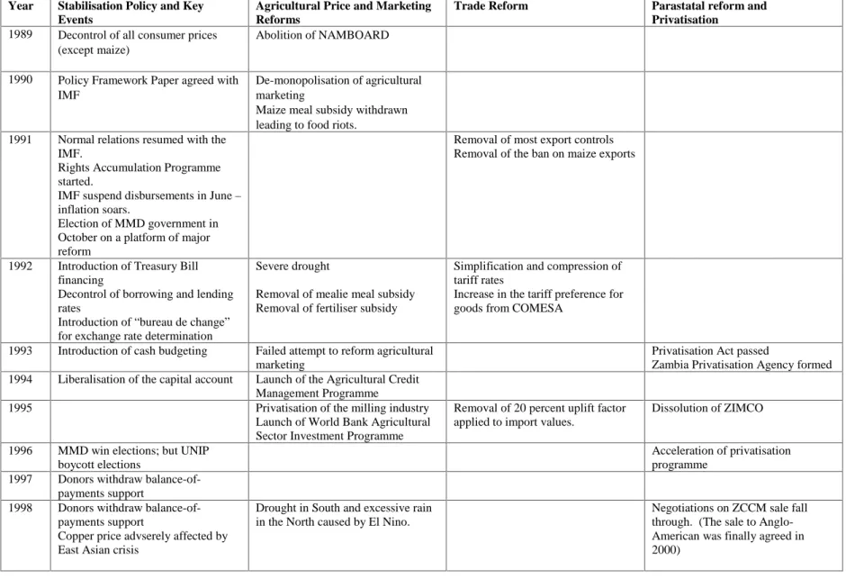
Table 1 shows a summary of the key policy reforms introduced over the 1990s along with the external shocks which affected the economy.

It is important to understand how these reforms have affected poverty and inequality in Zambia. In order to do so household data from three nationally representative surveys were analysed to determine the trends in poverty and inequality and to examine the different roles played by growth and distributional change in the evolution of poverty. The next section describes the household survey data used and the steps taken to ensure comparability over time – the following section describes the results.

Measuring Living Standards in Zambia

The most recent and accurate information on living standards in Zambia can be found from the four household surveys conducted in 1991, 1993, 1996 and 1998. The Zambian Central Statistical Office (CSO) conducted a Social Dimensions of Adjustment (SDA) Priority Survey9 between October 1991 and

November 1991 (Republic of Zambia 1993b). The survey was nationally representative covering all nine provinces and both urban and rural areas. The questionnaire covered demographic characteristics, health care, education, economic activities, housing facilities and amenities, access to facilities, migration, agriculture, non-farm enterprises, household income, household cash expenditure, household assets and anthropometry. In total 9,886 households were interviewed.

Between April and June 1993 a second SDA Priority Survey was undertaken covering the same topics and including 10,121 households (Republic of Zambia 1994b). Further, in 1996 a slightly expanded survey was undertaken entitled the Living Conditions Monitoring Survey (LCMS) (Republic of Zambia 1997c). This survey covered the same topics as the Priority Surveys but in addition asked questions about coping

9

strategies, migration, political participation and work by children. There was also a slight increase in the number of households interviewed to 11,752. Finally, between November and December 1998 another LCMS survey was undertaken initially sampling around 18,000 households.10

All of the surveys used a sampling frame drawn from the 1990 Census of Population and Housing and employed a similar multiple stage sample selection process. Although, Zambia is administratively divided into 9 provinces comprising 72 districts, the first three surveys only consider 57 of these districts because the other 15 had not been gazetted at that stage. However, all 72 districts were included in the 1998 survey. The CSO has delineated these districts into Census Supervisory Areas (CSAs) and Standard Enumeration Areas (SEAs). CSAs were selected in the first stage followed by Standard Enumeration Areas in the second stage and finally households at a third stage.11 Each district was allocated a minimum of 7 SEAs. In urban areas, SEAs were stratified according to low, medium and high cost housing areas. Within the selected rural SEAs, stratification was done on the basis of the scale of agricultural activity (small scale, medium scale, large-scale, and non-agricultural). These seven groups are mutually exclusive and hence any given household belongs to one and only one stratum.12

All four surveys were independent household surveys and thus interviewed different households in each year. Consequently it is not possible to construct a panel of households in order to examine the correlates and causes of changes in the welfare of individual households over time. The only exception to this is that half of the urban households interviewed in 1991 were also interviewed as part of the urban sample in 1993. Unfortunately subsequent data processing prior to our receipt of the data has made it extremely difficult to identify the same households across the two years. Consequently it has not been possible to construct a panel between any of the survey years.

The 1991, 1996 and 1998 surveys were conducted between October and December – this is the end of the hot dry season and the beginning of the hot wet season several months before the main harvest. In contrast, the 1993 survey was conducted between April and June – at the end of the hot wet season and the

beginning of the cold dry season. This is also around the time of the main harvest. Since annual

expenditure is based upon a one month recall period for most items and a two week recall period for food, consumption expenditures from the 1993 survey are not strictly comparable with expenditures from the other three surveys. Work by other researchers has shown that such time of survey biases can be severe (Dercon 1998). Consequently, we focus our analysis upon changes in poverty and inequality between the 1991, 1996 and 1998 surveys.

Unfortunately there were significant changes in the format and content of the income questions over the four surveys but the expenditure questions remained relatively unchanged. For both these and theoretic reasons, consumption expenditure was chosen as the welfare measure.13 In order to compare aggregate consumption expenditures across different years it is important that the measure reflects expenditure on the same items in each year. We therefore reconstructed a total expenditure variable for 1991, 1996 and 1998 including the following components: food, education, health, clothing, housing and transport. The inclusion (and exclusion) of items within any consumption aggregate is not uncontroversial since it can affect the conclusions drawn about whether aggregate consumption has increased or decreased among different segments of the population. We therefore briefly outline the choices which were made and the reasons for them – non-food items are considered first followed by a more detailed discussion of food expenditure.14

10

Although after data cleaning this fell to around 16,800 households.

11 For each survey, a household was defined as a group of persons who normally cook, eat and live together and regard

one person as the head of household.

12

There were minor changes to the stratification between the different surveys. See (Republic of Zambia 1993b) and (Cherel-Robson and McCulloch 2000) for details of the sampling methodology.

13

See (Ravallion 1992) for some of the arguments over the relative merits of income and consumption as welfare measures.

14

The education section of the 1991 questionnaire contains four sub-components of education expenditure: fees, uniforms, contribution to school PTA and private tuition. However, the data set only contains two education variables, fees and books. We therefore assume that these include all of the expenditures detailed in the questionnaire. In addition to the four sub-components included in 1991, the 1996 and 1998 questionnaires contain two other categories: "books" and "other school items". Although the latter is not explicitly mentioned in the 1991 questionnaire, it is plausible that households’ estimates of their education expenses include all items and hence, we include “other school items” in our measure of aggregate educational expenditure variable.15

Health expenditure in 1991 is an aggregate of a number of health related items. These items are broadly similar to the five sub-components included in the 1996 and 1998 surveys: medicines, hospital fees, traditional healing, hospitalisation and pre-payment scheme. The main exception is that expenditure on pre-payment health schemes is unlikely to be included in the estimate of 1991 health expenditure. We therefore exclude this from our estimates of aggregate health expenditure in each year to ensure

comparability. This is unlikely to seriously bias the results since expenditure on pre-payment schemes only constituted 5 percent of total health expenditure in 1998.

Questions regarding expenditure on clothing refer to the same items in each of the years (and explicitly exclude expenditure on school uniforms). However, there is a difference in recall periods between the different surveys: the 1991 questionnaire refers to expenditure during the last three months, whereas the 1996 and 1998 questionnaire refer to expenditure during the last month.

Housing expenditure in 1991 and 1996 includes: rent, water, electricity, candles, paraffin, charcoal, firewood, housing maintenance and other housing expenses. In addition to these catogories, the 1998 questionnaire includes expenditure on communication, TV, and telephone. We have assumed that these are accounted for in the "other housing expenses" category of the 1991 and 1996 questionnaires.

Expenditure on transport is broken into three categories in the 1991 questionnaire: expenditure on transport to work, expenditure on transport to school and “other kinds of transport”. The 1996 questionnaire employs a similar classification. The 1998 questionnaire is more detailed including sub-components on: transport to work, to school, to other places, and expenditure on fuel/oil, on vehicle repairs and on motorbike/boat repairs. Transport expenditure in 1991 represents 4.5 percent of total expenditure; including all of the components of transport expenditure in 1998 results in a transport share of total expenditure of 4.4 percent. We have therefore included all of these components in our aggregate measure of transport expenditure on the assumption they are included in the “other kinds of transport” category in 1991 and the “other transport expenses” category in 1996.16

The 1996 and the 1998 questionnaires are more detailed than the 1991 questionnaire, and hence some items had to be dropped from the calculation of total expenditure due to their non-inclusion in the 1991

questionnaire. These items are related to "personal services" such as cosmetics, laundry services, entertainment, domestic servants, cleaning material, alcohol and cigarettes. However, altogether they represented an average of only 8 percent of total household expenditure in 1998.

A total food expenditure variable was constructed based on food items which are listed in the 1991, 1996 and 1998 questionnaires. This means that, despite the fact that the 1998 food expenditure section is more comprehensive, we only consider the food items which are common to the three surveys. In addition the ways in which the questions on the consumption of vegetables, fruits, chicken and meat are asked differ

15

It is also worth noting that there is a difference in recall periods for education expenditure between the three surveys: the 1991 questionnaire asks questions about expenses during the past school year, whereas the 1996 questionnaire refers to expenses during the first and second school terms, and the 1998 data is based upon calculations of monthly education expenditure from all three school terms. We have no means of taking these differences into account and so we assume that these differences do not seriously bias our estimates of average monthly education expenditure.

16

Dropping variables related to expenditure on fuel/oil, on vehicle repairs and on motorbike/boat repairs would greatly reduce our estimate of transport expenditure in 1998 since these items average 28.1, 22.6 and 3.7 percent of total household transport expenditure in 1998 respectively.

between the surveys. We have therefore chosen the sub-categories of each food which are most likely to be comparable across surveys (Cherel-Robson and McCulloch 2000).

More importantly, the consumption of own produced food is accounted for differently in 1991 than in 1996 and 1998. The documentation of the 1991 survey states that no data was collected on own consumption (Republic of Zambia 1993b). Despite this, the expenditure dataset contains a variable labeled "Imputed own consumption" but it is not clear how this variable was computed. The 1996 and 1998 surveys did explicitly ask about consumption from own production. Given that consumption from own production is extremely important to the poor it is not possible simply to drop own consumption from our aggregate expenditure measure. In fact, most of the own consumption values reported in each of the surveys are plausible and so we construct a total food expenditure value for each household which consists of the sum of food purchases, food received and consumption of own produced food (that is, although the

classification of purchases, received and own produced food into the available variables may not be clear in all the data sets, we assume that the sum of the available food consumption variables in each year contains all these elements.)

In one case however this is clearly unsatisfactory. A small number of households in each year have very low or zero values for food expenditure. While having a zero value for own consumption is plausible (for urban households who produce no food) and a zero value for purchased and received food consumption is possible for very poor subsistence households, it is not credible that households maintain zero consumption on all food over a long period of time. The problem is particularly severe in 1991 which has 152 rural households and 400 urban households with implausibly low food expenditure. Including these households results in a marked downwards shift in the consumption distribution. This means that when 1991 is compared with 1996 and 1998 the position of the very poorest households appears to have improved markedly simply because fewer households in 1996 and 1998 have spurious low values for food expenditure. We have therefore dropped these 552 households from our analysis in 1991.17

In order to compare welfare across households with different compositions we employ the equivalence scale used by (Latham 1965). This scale is slightly different from the one used by the Zambian CSO – consequently per adult equivalent consumption expenditure was recalculated using the Latham scale. The scale is shown in Appendix 1.

Finally, to calculate poverty measures we have used the poverty line defined by the Zambian Central Statistical Office which is based upon a cost of basic needs approach. A study carried out by the National Food and Nutrition Commission constructed a basic food basket necessary to maintain the nutritional requirements of an average Zambian family.18 The cost of this food basket translates into a lower poverty line of K961 per adult person per month in 1991 prices. A further 30 per cent was added to this amount to account for basic non-food needs, giving an upper poverty line of K1,380 per month. These values were first upgraded to 1998 prices using the ratio of the composite national consumer price index in December 1998 to that in October 1991 (Republic of Zambia 2000; Republic of Zambia 1997a) and then adjusted to account for the difference between the CSO and Latham equivalence scales to give K32,232.85 and K46,286.50 for the two poverty lines.19

For purposes of international comparison a US$1 per day poverty line was also calculated using the PPP exchange rates in the Penn World Tables (Summers and Heston 1999) and the Zambian Consumer Prices Index (Republic of Zambia 1997a). This resulted in a per capita “poverty” line of K140,642.04 per month in 1998 prices. This is exceptionally high in a Zambian context being in the top decile of the 1998 consumption expenditure distribution. It was therefore decided not to use this poverty line in our analysis.

17 An alternative approach to this problem would be to estimate the consumption expenditure of the 552 households

with implausibly low values for food expenditure. A reduced form consumption equation could be estimated using information about households’ demographic composition, educational attainment and asset ownership.

18

The food basket comes from (ILO/JASPA 1981).

19

(Cherel-Robson and McCulloch 2000) gives the details of this adjustment. The use of a different equivalence scale means that some of our results are different from those produced by the Zambian CSO – however the overall pattern of results is similar.

Changes in Poverty and Inequality Over Time in Zambia

The data from all three of the surveys outlined above were re-analysed to explore how poverty and inequality have changed over the 1990s. For conciseness only results based upon per adult equivalent expenditure are reported; similar results were obtained using per capita expenditure measures. Table 2 shows the mean per adult equivalent consumption expenditure for 1991, 1996 and 1998 – all figures are in 1998 Kwacha. Population standard errors are reported which take into account the stratification and clustering of the surveys.

The table shows a decline of over 20 percent in the population real mean expenditure between 1991 and 1996. Although urban residents are substantially better off than rural residents, Table 2 shows that most of this fall comes from a sharp, and statistically significant, fall of over a fifth in the mean expenditure of households in urban areas. The mean expenditure of rural residents actually increases by 13 percent between 1991 and 1996, although this is from a much lower base and the change is not statistically significant.

By contrast, between 1996 and 1998 the national mean per adult equivalent consumption expenditure increased by over a third. Most of this increase resulted from a large and statistically significant increase of 62 percent in rural mean expenditure. The mean consumption expenditure of urban residents also rose slightly between 1996 and 1998, although the change was not statistically significant. Because of these increases, the mean expenditure of rural residents was over 80 percent higher in 1998 than in 1991. However, urban residents were on average a fifth worse off in 1998 than in 1991.

Cumulative Density Functions

Whilst Table 2 shows the means of the expenditure distributions for each year, it is more informative to examine the entire distribution. This can be done by plotting the Cumulative Density Function (CDF) of consumption expenditure for each year. Figure 5a shows the CDFs for 1991, 1996 and 1998 plotted together with the lower and upper poverty lines (K32,232.85 and K46,286.50 per adult equivalent per month respectively). The vertical axis shows the proportion of the population with per adult equivalent expenditure below the value given on the horizontal axis. Thus the intersection of the CDF with the vertical line drawn at the value of per adult equivalent expenditure equal to the poverty line, gives the percentage of the population with per adult equivalent expenditure less than the poverty line – that is – the poverty headcount.

The CDF for 1996 lies above that of 1991 at both poverty lines indicating a rise in the poverty headcount between these two years. The poverty headcount using the upper poverty line was 69.5 percent in 1991 – this had risen to over 80 percent by 1996. However, Figure 5a also shows the CDF for 1998 lying some distance below that for 1996. This shows a reduction in poverty between these two years with the headcount falling from 81 percent to 72 percent.

If a CDF for one year is always above or to the left of the CDF for another then this means that poverty will be higher for that year than for the other year using any well-behaved poverty measure, a property known as first-order stochastic dominance (Ravallion 1992). If however, the CDFs cross then it is possible for poverty in one year to be higher than in the other year when using one poverty measure, but lower if another poverty measure is chosen. The CDF of 1991 crosses the CDF of 1996 at a value of per adult equivalent expenditure per month of around one half of the lower poverty line. This suggests that, despite the large increase in the poverty headcount, the proportion of the population in extreme poverty declined between 1991 and 1996. However we treat this result with some caution due to the problems described above with the unreliability of the recorded values for consumption at the bottom of the expenditure distribution in 1991.

The CDF for 1991 crosses the CDF for 1998 above the lower poverty line. Thus although the poverty headcount increases slightly between the two years using the upper poverty line, it decreases slightly using the lower poverty line. Furthermore, we would expect the poverty gap and squared poverty gap measures to show a substantial decline between 1991 and 1998, although again some caution may be needed in accepting these results. However, the 1998 CDF lies below that of 1996 throughout the entire distribution – thus any poverty measure or poverty line would find a reduction in poverty between these two years.

It is also instructive to look at the rural and urban expenditure distributions separately. Figure 5b shows the CDFs for the rural expenditure distributions between 1991, 1996 and 1998, whilst Figure 5c shows the CDFs for the urban expenditure distribution between the same years. Around the two poverty lines, the CDF for the rural distribution in 1996 lies almost on top of that for 1991, indicating that the poverty headcount changed very little over this period (lower down the distribution there appears to be a fall in poverty between 1991 and 1996 but for the reasons mentioned above we do not attach great confidence to this result). However, the rural CDF for 1998 lies well below that of 1996 and 1991 for all values of poverty line. Consequently the observed improvement in rural poverty between 1996 and 1998 is robust to the choice of poverty line.

The CDFs for the urban expenditure distributions shown in Figure 5c are much “shallower” than those for rural areas since the percentage of the population below both poverty lines is much lower in urban areas than in rural areas. Nonetheless, Figure 5c shows a substantial increase in poverty between 1991 and 1996 with the poverty headcount rising from 47 percent to 65 percent. The CDF for 1998 lies fractionally below that for 1996 indicating a small improvement between these two years in urban areas.

Calculation of Population Poverty Estimates

Population estimates of poverty were calculated using the Foster, Greer, Thorbecke poverty measures (Foster, Greer et al. 1984) with α = 0,1 and 2 – these correspond to the poverty headcount, the poverty gap and the squared poverty gap. The two national poverty lines20 of K32,232.85 and of K46,286.50 per adult equivalent per month in 1998 prices were used.

Table 3a shows the population estimates of poverty for 1991, 1996 and 1998. As predicted by the CDFs the poverty headcount using the upper poverty line rose between 1991 and 1996 from 69 percent to 81 percent, but then fell to 72 percent in 1998; the same pattern was observed using the lower poverty line. The poverty gap and the squared poverty gap followed a similar pattern, increasing between 1991 and 1996 and decreasing between 1996 and 1998 (although the squared poverty gap using the lower poverty line fell slightly between 1991 and 1996).

Although Zambia is, by sub-Saharan African standards, a very urbanised society, 63 per cent of the population live in rural areas. It is therefore useful to breakdown the analysis of poverty in rural and urban strata. Table 3b shows the poverty headcount, poverty gap and squared poverty gap in each year for rural and urban areas separately. There has been a substantial change in the geographical prevalence of poverty in Zambia over the 1990s. In 1991 poverty was far more prevalent in rural areas than in urban areas; the poverty headcount in rural areas for the upper poverty line was almost 90 percent while in urban areas it was 47 percent. However, the increase in urban poverty over the decade combined with the improvement in the rural standard of living between 1996 and 1998 has resulted in a rural poverty headcount of 77 percent compared with an urban poverty headcount of 63 percent in 1998. Urban areas are still better off than rural ones – but the difference has been narrowed.

In rural areas, the poverty headcount remained at around 89 percent between 1991 and 1996, but then fell to 77 percent in 1998 – mirroring the national trend. However, the poverty gap and the squared poverty gap fell significantly throughout the 1990s, as predicted from the rural CDFs. By contrast, in urban areas there was a dramatic increase in all three poverty measures between 1991 and 1996. Subsequently there

20

has been a slight reduction in the poverty headcount between 1996 and 1998, but little significant change in either the poverty gap or the squared poverty gap.

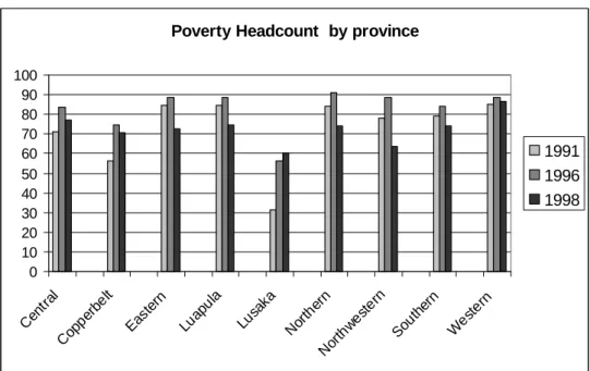
It is also instructive to examine the incidence of poverty across different regions and socio-economic groups. Figure 6a shows the poverty headcount for each of the nine provinces for 1991, 1996 and 1998 using the upper poverty line of K46,286 per adult equivalent. The proportion of the population below the poverty line increased in every province between 1991 and 1996. The largest increases in the poverty headcount between 1991 and 1996 occurred in the most urbanised provinces - Lusaka, Central and Copperbelt – consistent with the picture of rising urban poverty shown in Table 3b. Further, these provinces saw little or no reduction in their poverty headcount between 1996 and 1998 with the result that poverty headcounts in these provinces were much higher in 1998 than in 1991. In Lusaka in particular the poverty headcount has almost doubled since 1991. Nonetheless, all provinces except Lusaka saw a decrease in the poverty headcount between 1996 and 1998 with the result that the poverty headcount was lower in 1998 than in 1991 in five provinces – all predominantly rural – and higher in four (all

predominantly urban except for Western province).

The improvement in poverty in rural provinces is also reflected in Figure 6b which shows the squared poverty gap for each province and year. The severity of poverty in 1991 is highest in Eastern, Luapula, Northern, North-Western, Southern and Western provinces. However, all of these provinces saw consistent and substantial falls in their squared poverty gap between 1991 and 1998. However, in Lusaka and the Copperbelt the squared poverty gap doubled over the same period.

The large reductions in the squared poverty gap for most provinces suggest that the changes experienced have been relatively pro-poor. To explore this further we examined the growth in per adult equivalent consumption expenditure for each decile of the expenditure distribution – these are shown in Figure 7. Between 1991 and 1996 the bottom four deciles of the distribution show positive consumption growth, with the bottom three deciles growing very strongly. By contrast, the next five deciles experience a contraction in their consumption expenditure, with larger reductions being experienced by households with higher expenditure, although the very richest manage to avoid a fall in their mean consumption expenditure. A similarly pro-poor pattern of growth emerges for the changes from 1996 to 1998, with all deciles experiencing an increase in mean expenditure and poorer deciles having larger percentage increases than richer ones.

Whilst examining changes in poverty by decile reveals much about the pattern of growth, deciles

themselves often do not constitute a useful grouping for policy analysis. It is therefore helpful to examine the changes in poverty by socio-economic group. None of the surveys constructed a detailed classification of households by socio-economic group, but the surveys were stratified by four household types in rural areas (small, medium and large-scale agricultural, and non-agricultural) and by the quality of residential area (low, medium and high cost) in urban areas. Figure 8 presents the poverty headcount by these strata. The incidence of poverty in 1991 was highest amongst small and medium scale agricultural households and remained high in 1996. However there was a substantial fall in the poverty headcount for these strata between 1996 and 1998.21 The poverty headcount for rural non-agricultural households increased substantially between 1991 and 1996, but then fell between 1996-1998 in keeping with all the other rural strata.

The situation for the urban strata was quite different. Poverty rose in all three urban strata between 1991 and 1996. Between 1996 and 1998 poverty in low cost areas remained roughly constant, whilst in medium cost areas it continued to rise. By contrast in high cost areas poverty fell, perhaps reflecting the ability of relatively wealthy households to protect themselves from declines in consumption.

21

The large rise and then decline in the poverty headcount for large scale agricultural households may not be

Inequality Measures

In order to assess the extent to which the distribution of consumption expenditure changed over the 1990s, a number of inequality measures were calculated for all three years. To check the robustness of the results to the choice of measure, five different measures were used: the coefficient of variation; standard deviation of logs; Gini coefficient; Theil’s Entropy measure; and Theil’s mean log deviation. Each of these measures emphasises different parts of the distribution (see (Cowell 1995) for an exposition of their properties).

Table 4 shows that there was a drop in inequality between 1991 and 1996 with the Gini coefficient falling from 0.559 to 0.518. This drop occurs regardless of the inequality measure used, although the fall is much larger for the coefficient of variation than for the other inequality measures suggesting that movements in the tails of the expenditure distribution were responsible for much of the change. A further, smaller drop in inequality was experienced between 1996 and 1998, with the Gini falling to 0.509.

Table 4 also shows inequality measures for the rural and urban consumption expenditure distributions separately. Rural inequality declined between 1991 and 1996 for all inequality measures except the coefficient of variation. However, between 1996 and 1998, rural inequality increased by all measures except the coefficient of variation. Thus, notwithstanding changes in the tails of the distribution to which the coefficient of variation is particularly sensitive, an initial fall in inequality between 1991 and 1996 has been counteracted by a subsequent rise as growth picked up in rural areas.

The evolution of urban inequality over the 1990s is more complex. Inequality rose between 1991 and 1996 according to the Gini coefficient, the Theil entropy measure and the mean log deviation; but it fell

according to the coefficient of variation and the standard deviation of logs. Similarly, between 1996 and 1998 three measures report an increase in inequality whilst two report a decrease. Overall the changes in the urban expenditure distribution were small and of ambiguous sign. However, despite most inequality measures showing an increase in inequality within both rural and urban areas between 1996 and 1998, national inequality fell over this period. This is because inequality between the rural and urban areas declined as expenditure in rural areas grew much faster than in urban areas.

Table 5 calculates the inequality measures for each province and shows a number of variations from the national picture. Most provinces show strong declines in inequality between 1991 and 1996. However, Luapula, Lusaka and the Copperbelt have large increases in inequality over the period. Similarly, Central, Copperbelt, Southern, and North-western provinces all show an increase in inequality between 1996 and 1998, while all other provinces show declines.

A fuller picture of the changes in the expenditure distribution can be obtained by looking at the Lorenz curves for 1991, 1996 and 1998. The Lorenz curve shows the proportion of the total expenditure on the vertical axis spent by the proportion of the population on the horizontal axis. Thus if all individuals had the same expenditure the curve would be a straight line from the origin to the top right hand corner of the graph. Alternatively the situation in which one person spent the entire national expenditure with all others spending nothing would be indicated by a line running along the horizontal axis jumping up to one only for the last (very rich) person. Thus by plotting Lorenz curves for the different years it is possible to see how the distribution of expenditure has changed independently from the mean expenditure.

If a Lorenz curve for one year lies everywhere above the Lorenz curve for another year then it is possible to say that inequality has been reduced (that is, all conventional inequality measures will show a reduction). However, if the Lorenz curves for two years cross then this indicates that one part of the distribution may have improved (e.g. the distribution of expenditure of the poor) whilst another may have worsened. Figure 9a shows the Lorenz curves for 1991, 1996 and 1998 together. These show that the 1996

expenditure distribution was more equal at almost all points than the 1991 distribution consistent with the substantial drop in most measures of inequality between these two years. However, the Lorenz curve for 1991 crosses that for 1996 at the very top of the distribution indicating that inequality increased at the top of the distribution; this may explain the movement of the coefficient of variation which places emphasis upon changes in the tails of the distribution. The Lorenz curve for 1998 lies slightly inside that for 1996 explaining the small declines in national inequality shown by all measures.

Figures 9b and 9c show the Lorenz curves for rural and urban areas respectively for all three years. The rural Lorenz curve confirms the impression gained from Table 4 of a decline in inequality between 1991 and 1996 except at the very top of the distribution. However the rural Lorenz curve for 1998 lies clearly outside that for 1996 explaining the increase in inequality between these two years. The Lorenz curves for urban areas show almost the reverse position, with an increase in inequality between 1991 and 1996, but no corresponding decline during the subsequent two years.

Has growth or distributional change been responsible for the changes in poverty?

The increase in poverty between 1991 and 1996 occurred despite a remarkable equalisation of the national distribution of consumption between these years. Similarly, the reduction in poverty between 1996 and 1998 coincided with an increase in inequality in rural areas. This suggests that growth (or recession) has been primarily responsible for the changes in poverty. It is possible to quantify the relative importance of the roles played by growth and changes in distribution by decomposing changes in poverty into growth and inequality components (Ravallion and Datt 1992). Thus the change in poverty between two periods can be represented by the sum of three components:

(1) a growth component: this is the change in poverty which would have occurred if the growth in the average expenditure had occurred without any change in the initial distribution of expenditure; (2) an inequality component: this is the change in poverty which would have occurred if the distribution

of expenditure had shifted from its initial distribution to its final distribution without any change in the average expenditure; and

(3) a residual: this is equal to the difference between the growth components measured at the final and initial expenditure distributions.22

If the growth component is the largest part of the change in poverty then this indicates that growth has played a more important role than distribution in achieving the change in poverty and vice versa.

Table 6a shows poverty decompositions for the headcount, poverty gap and squared poverty gap poverty measures for the change in poverty between 1991 and 1996 and between 1996 and 1998. The

decompositions shown use a modification to the Datt and Ravallion decomposition by Kakwani (Kakwani 1997) which dispenses with the need for a residual term by averaging results across the initial and final distributions and means.23

For the headcount measure of poverty the results show that, for both poverty lines, the increase in the headcount between 1991 and 1996 was caused principally by the downward shift in mean expenditure. Of the 12 percent change in the poverty headcount – eight percent was due to sharp recession between these two years, whilst 4 percent was due to the change in the distribution of consumption. It may seem surprising that the improvement in distribution of consumption between 1991 and 1996 would still have caused an increase in the poverty headcount even if mean expenditure had remained unchanged. This is a consequence of the very high incidence of absolute poverty in Zambia so that both poverty lines are above median expenditure. An improvement in the distribution caused by taking resources from a better off household and giving it to a worse off one could therefore move the better off household below the poverty line increasing the headcount.

The same anomaly does not apply to the decomposition using the poverty gap and squared poverty gap measures. With these we observe the damaging impact of the contraction in mean expenditure being counteracted by the improvement in the distribution between 1991 and 1996. Indeed with the squared poverty gap measure, the improvement in the distribution negates the effect of the recession with the result that the squared poverty gap falls slightly with the lower poverty line. Between 1996 and 1998 there is

22

Equivalently it is the difference between the inequality components measured at the final and initial mean expenditures.

23