Are Bayesian Networks Sensitive to Precision of
Their Parameters?
Marek J. Dru˙zd˙zel1,2 and Agnieszka Oni´sko1,3
1 Faculty of Computer Science, Bia lystok Technical University, Wiejska 45A, 15-351 Bia lystok, Poland
2 Decision Systems Laboratory, School of Information Sciences and Intelligent Systems Program, University of Pittsburgh, Pittsburgh, PA 15260, USA
3 Magee Womens Hospital, University of Pittsburgh Medical Center, Pittsburgh, PA 15260, USA
Abstract
In this paper, we examine whether Bayesian networks are sensitive to precision of their parameters in the context ofHepar II, a sizeable Bayesian network model for diagnosis of liver disorders. Rather than entering noise into probability distribu-tions, which was done in prior studies, we change their precision, starting with the original values and rounding them systematically to progressively rougher scales. It appears that the diagnostic accuracy ofHepar IIis very sensitive to imprecision in probabilities, if these are rounded. However, the main source of this sensitivity appears to be in rounding small probabilities to zero. When zeros introduced by rounding are replaced by very small non-zero values, imprecision resulting from rounding has minimal impact on Hepar II’s performance.
Keywords: Bayesian networks, knowledge engineering, uncertainty management
1 Introduction
Decision-analytic methods provide an orderly and coherent framework for mod-eling and solving decision problems in decision support systems (Henrion et al., 1991). A popular modeling tool for complex uncertain domains is a Bayesian net-work (Pearl, 1988), an acyclic directed graph quantified by numerical parameters and modeling the structure of a domain and the joint probability distribution over its variables. There exist algorithms for reasoning in Bayesian networks that typi-cally compute the posterior probability distribution over some variables of interest given a set of observations. As these algorithms are mathematically correct, the ultimate quality of reasoning depends directly on the quality of the underlying models and their parameters. These parameters are rarely precise, as they are often based on subjective estimates. Even when they are based on data, they may not be directly applicable to the decision model at hand and be fully trustworthy. Search for those parameters whose values are critical for the overall quality of decisions is known as sensitivity analysis. Sensitivity analysis studies how much a model output changes as various model parameters vary through the range of their
plausible values. It allows to get insight into the nature of the problem and its formalization, helps in refining the model so that it is simple and elegant (contain-ing only those factors that matter), and checks the need for precision in refin(contain-ing the numbers (Morgan and Henrion, 1990). It is theoretically possible that small variations in a numerical parameter cause large variations in the posterior proba-bility of interest. Van der Gaag and Renooij (2001) found that real networks may indeed contain such parameters. Because practical networks are often constructed with only rough estimates of probabilities, a question of practical importance is whether overall imprecision in network parameters is important. If not, the ef-fort that goes into polishing network parameters might not be justified, unless it focuses on their small subset that is shown to be critical.
There is a popular belief, supported by some anecdotal evidence, that Bayesian network models are overall quite tolerant to imprecision in their numerical param-eters. Pradhanet al.(1996) tested this on a large medical diagnostic model, the CPCSnetwork (Middletonet al., 1991; Shwe et al., 1991). Their key experiment focused on systematic introduction of noise in the original parameters (assumed to be the gold standard) and measuring the influence of the magnitude of this noise on the average posterior probability of the true diagnosis. They observed that this average was fairly insensitive to even very large noise. This experiment, while ingenious and thought provoking, had several weaknesses. In our earlier work (Oni´sko and Druzdzel, 2003), we replicated the experiment of Pradhan et al. usingHepar II, a sizeable Bayesian network model for diagnosis of liver disorders. We systematically introduced noise inHepar II’s probabilities and tested the di-agnostic accuracy of the resulting model. Similarly to Pradhan et al., we assumed that the original set of parameters and the model’s performance are ideal. Noise in the original parameters led to deterioration in performance. The main result of our analysis was that noise in numerical parameters started taking its toll almost from the very beginning and not, as suggested by Pradhan et al., only when it was very large. The region of tolerance to noise, while noticeable, was rather small. That study suggested that Bayesian networks may be more sensitive to the quality of their numerical parameters than popularly believed.
The question of sensitivity of Bayesian networks to precision of their parameters is of much interest to builders of intelligent systems. In precision does not matter, qualitative “order of magnitude” schemes should perform well without the need for precise, numerical estimates. Conversely, if network results are sensitive to the precise values of probabilities, it is unlikely that a qualitative approach will ever match the performance of a quantitative problem specification.
This paper describes a follow-up study that probes the issue further. We examine a related question: “Are Bayesian networks sensitive to precision of their parameters?” Rather than entering noise into the parameters, we change their precision, starting with the original values and rounding them systematically to progressively rougher scales. This models a varying degree of precision of the parameters. One difficulty that comes with rounding probabilities is that these do not necessarily add up to 1.0 after rounding. Fortunately, there is a well-developed mathematical theory of rounding proportions that we base our approach on. Our results show that the diagnostic accuracy of Hepar II is very sensitive to imprecision in probabilities, if these are rounded. However, the main source of
this sensitivity appears to be in rounding small probabilities to zero. When zeros introduced by rounding are replaced by very small non-zero values, imprecision resulting from rounding has almost no impact onHepar II’s performance.
The remainder of this paper is structured as follows. Section 2 provides a brief review of relevant literature on the topic of rounding probabilities. Section 3 introduces theHepar IImodel. Section 4 describes the results of our experiments. Finally, Section 5 discusses our results in light of previous work.
2 Rounding of probability distributions
Approximating a number amounts to rounding it to a value that is less precise than the original value. For example, according to the year 2000 census, the population of the United States was 281,421,906. This number can be expressed in different units, for example as 281,421.906 thousand or as 281.421906 million, rounded to 281,422 thousand or to 281 million respectively, each successive rounding leading to some loss of precision. While several rounding rules exist, the most common, applied to the example above, rounds the fractional part to the nearest integer.
Rounding probabilities and, in general, proportions can be approached simi-larly, although there is an additional complication. If we round a set of proportions using a standard rounding method, their sum will not necessarily equal to 1.0. In fact, as the number of categories approaches infinity, the probability that the sum of their rounded weights is equal to 1.0 approaches zero (Mosteller et al., 1967). This problem has been studied for at least two centuries with basic anal-ysis conducted around the time of the design of the United States constitution. A moderately rich literature on the topic exists that studies various algorithms for ensuring that the sum of rounded proportions does add to 1.0. Balinski and Young (1982), in their excellent monograph, prove that among all rounding proce-dures only quotient methods (also calledmultipler methods) are free from irritating paradoxes.
For our experiment, we selected a generic stationary rounding algorithm for proportions based on a multiplier method, as described in Heinrich et al.(2005) and summarized below. The algorithm has three parameters: (1) stationarity parameter q (most common value used in rounding is q = 0.5), (2) accuracy n
(this is the number of intervals that the proportions are to be expressed in, so
n= 10 gives us the accuracy of 0.1), and (3) a global multiplier ν (the value ofν
is typically chosen to be ν=n).
Let (w1, w2, . . . , wc) be a vector ofcweights. The algorithm focuses on finding a vector of integer numerators (Nq,1, Nq,2, . . . , Nq,c), such that P
c
i=1Nq,i = n, that uniquely determines the rounded weights. To derive a rounded weightwq,iit is sufficient to divide Nq,i byn. To obtain the numerators Nq,i, i= 1, . . . , c, we first compute thediscrepancyD
D= X j≤c [νwj]q −n ,
which is a random variable with integer values in the interval (ν−n−cq, ν−n+
the final numerators
Nq,j = [νwj]q−sgn(D)mj,n(D),
where mj,n(D) is the count of how often indexj appears among the|D|smallest quotients
( k−νwi+[νwi]q+q−1
wi fori= 1, . . . , candk= 1, . . . ,−D; whenD <0 ;
k+νwi+[νwi]q−q
wi fori= 1, . . . , candk= 1, . . . , D; whenD >0. Example 1 Let (0.04,0.14,0.46,0.36) be a vector of 4 weights and the desired accuracy ben= 10. We conveniently setν=n= 10and use the standard value of the rounding parameterq= 0.5. This yields the initial values of numeratorsνw= (0,1,5,4)and the value of discrepancyD= 0. No adjustment to the numerators is needed and we obtain the vector of rounded weights of(0.0,0.1,0.5,0.4)by dividing each of the numerators by n= 10.
Example 2 However, an initial vector of weights(0.04,0.14,0.48,0.34)yields the initial values of numeratorsνw= (0,1,5,3)and the value of discrepancyD=−1. Using the formula for D < 0, we compute the quotients of (2.5,0.71,1.08,0.29) and adjust w4 (the smallest of the quotients was for i = 4) by 1, yielding D = 0, the final vector of numerators (0,1,5,4) and the resulting rounded weights of (0.0,0.1,0.5,0.4).
3 The
Hepar II
model
Our experiments are based onHepar II(Oni´skoet al., 2001), a Bayesian network model consisting of over 70 variables modeling the problem of diagnosis of liver disorders. The model covers 11 different liver diseases and 61 medical findings, such as patient self-reported data, signs, symptoms, and laboratory tests results. The structure of the model, (i.e., the nodes of the graph along with arcs among them) was built based on medical literature and conversations with domain experts and it consists of 121 arcs. There are on the average 1.73 parents per node and 2.24 states per variable. The numerical parameters of the model (there are 2,139 of these in the most recent version), i.e., the prior and conditional probability distributions, were learned from a database of 699 real patient cases. Readers interested in theHepar II model can download it from Decision Systems Laboratory’s model repository athttp://genie.sis.pitt.edu/.
As our experiments study the influence of precision ofHepar II’s numerical parameters on its accuracy, we owe the reader an explanation of the metric that we used to test the latter. We focused on diagnostic accuracy, which we defined in our earlier publications as the percentage of correct diagnoses on real patient cases. When testing the diagnostic accuracy ofHepar II, we were interested in both (1) whether the most probable diagnosis indicated by the model is indeed the correct diagnosis, and (2) whether the set of wmost probable diagnoses contains the correct diagnosis for small values of w (we chose a “window” of w=1, 2, 3, and 4). The latter focus is of interest in diagnostic settings, where a decision
support system only suggest possible diagnoses to a physician. The physician, who is the ultimate decision maker, may want to see several alternative diagnoses before focusing on one.
With diagnostic accuracy defined as above, the most recent version of the Hepar IImodel reached the diagnostic accuracy of 57%, 69%, 75%, and 79% for window sizes of 1, 2, 3, and 4 respectively (Oni´skoet al., 2002).
4 Experimental results
We have performed three experiments to investigate how progressive rounding of Hepar II’s probabilities affects its diagnostic performance. To that effect, we have successively created various versions of the model with different precision of parameters and tested the performance of these models. The following two sections describe the rounding process and the observed results respectively.
4.1 Progressive rounding of Hepar II parameters
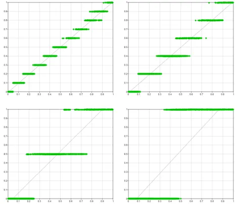
For the purpose of our experiment, we use the values of n = 100, 10, 5, 4, 3, 2, and 1. As the reader may recall from Section 2, these correspond to the number of intervals in which the probabilities fall. And so, whenn= 10, the probability space is divided into 10 intervals and each probability takes one of 11 values, i.e., 0.0, 0.1, 0.2, . . . , 0.9, and 1.0. When n = 5, each probability takes one of six values, i.e., 0.0, 0.2, 0.4, 0.6, 0.8, and 1.0. When n = 2, each probability takes one of only three values, i.e., 0.0, 0.5, and 1.0. Finally, whenn= 1, the smallest possible value of n, each probability is either 0.0 or 1.0. Figure 1 shows scatter plots of all 2,139 Hepar II’s parameters (horizontal axis) against their rounded values (vertical axis) fornequal to 10, 5, 2, and 1.
Please note the drastic reduction in precision of the rounded probabilities, as pictured by the vertical axis. Whenn= 1, all rounded probabilities are either 0 or 1. Also, note that the horizontal bars in the scatter plot overlap. For example, in the upper-right plot (n= 5), we can see that an original probabilityp= 0.5 in Hepar II got rounded sometimes to 0.4 and sometimes to 0.6. This is a simple consequence of the surrounding probabilities in the same distribution and the necessity to make the sum of rounded probabilities add to 1.0, as guaranteed by the algorithm.
4.2 Effect of imprecision on Hepar II’s diagnostic performance
For the purpose of our experiments, we assumed that the model parameters were perfectly accurate and, effectively, the diagnostic performance achieved was the best possible. In the experiments, we study how this baseline performance de-grades under the condition of noise. Of course, in reality the parameters of the model may not be accurate and the performance of the model can be improved upon.
Figure 1: Rounded vs. original probabilities for various levels of rounding accuracy.
4.2.1 Experiment 1
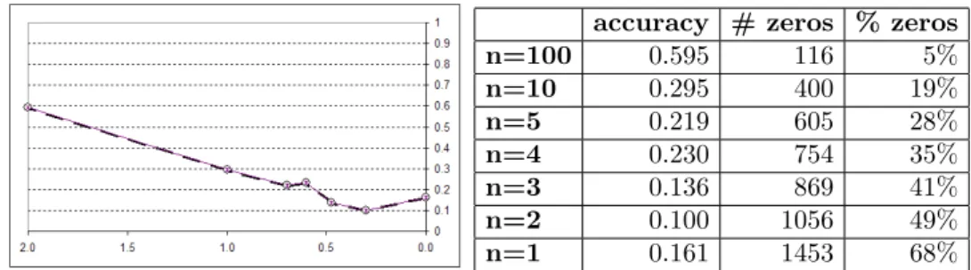
In our first experiment, we computed the diagnostic accuracy of various versions ofHepar II, as produced by the rounding procedure. Figure 2 shows a summary of the results in both graphical and tabular format. The horizontal axis in the plot corresponds to the number of intervalsnin logarithmic scale, i.e., value 2.0 corre-sponds to the roundingn= 100, and value 0 to the roundingn= 1. Intermediate points, for the other roundings can be identified in-between these extremes.
The plot shows clearly that the accuracy of the system goes down exponentially (as testified by an almost straight line in logarithmic scale). We investigated this further and came to the following conclusion. The algorithm presented in Section 2 rounds proportions on a linear scale. A small absolute difference between two proportions is treated in the same way, regardless of whether it is part of a large fraction or it is close to zero. In Example 2, the algorithm rounded 0.14 to 0.1, 0.34 to 0.3, and at the same time 0.04 to 0.0. While the first two rounding make perfect sense, the last one, i.e., rounding 0.04 to zero is quite a drastic step. Zero probability is a very special value in probability theory, as it denotes an impossible event. A quick examination of Bayes theorem will show that once an event is found to be of zero probability, it stays impossible, no matter how strong the evidence in its favor. This has serious practical consequences for a system based essentially
accuracy # zeros % zeros n=100 0.595 116 5% n=10 0.295 400 19% n=5 0.219 605 28% n=4 0.230 754 35% n=3 0.136 869 41% n=2 0.100 1056 49% n=1 0.161 1453 68%
Figure 2: Diagnostic performance ofHepar IIas a function of logarithm of parameter
accuracy (w=1).
on Bayes theorem. It can be shown that the rounding algorithm will turn most probabilities that are smaller than 1/(2n) into zero. As the right-most two columns in Figure 2 show, there is an increasing number of them as precision decreases.
4.2.2 Experiment 2
We addressed this problem by replacing all zeros introduced by the algorithm by small ε probabilities and subtracting the introduced εs from the probabilities of the most likely outcomes in order to preserve the constraint that the sum should be equal to 1.0. While this caused a small distortion in the probability distributions (e.g., a value of 0.997 instead of 1.0 when ε= 0.001 and there were three induced zeros transformed into ε), it did not introduce sufficient difference to invalidate the precision loss. To give the reader an idea of what it entailed in practice, we will reveal the so far hidden information that the plots in Figure 1 were obtained for data withε= 0.001.
ε=0.01 0.001 0.0001 n=100 0.596 0.595 0.596 n=10 0.586 0.582 0.578 n=5 0.585 0.575 0.559 n=4 0.576 0.569 0.548 n=3 0.554 0.546 0.529 n=2 0.515 0.515 0.506 n=1 0.479 0.479 0.476
Figure 3: Diagnostic performance ofHepar IIas a function of logarithm of parameter
accuracy andε(w=1).
The result of this modification was dramatic and is pictured in Figure 3, each line for a different value ofε(we preserved the result of Experiment 1 in the plot). The meaning of the horizontal and vertical axes is the same as in Figure 2. As can be seen, the actual value ofεdid not matter too much (we tried three values: 0.0001, 0.001, and 0.01). In each caseHepar II’s performance was barely affected,
even when there was just one interval, i.e., when all probabilities were eitherεor 1−ε.
4.2.3 Experiment 3
Our next experiment focused on the influence of precision in probabilities on Hepar II’s accuracy for windows of size 1, 2, 3, and 4. Figure 4 shows a summary of the results in both graphical and tabular format. The meaning of the horizontal and vertical axes is the same as in Figures 2 and 3. We can see that the stability ofHepar II’s performance is similar for all window sizes.
w=1 w=2 w=3 w=4 n=100 0.595 0.721 0.785 0.844 n=10 0.582 0.708 0.778 0.823 n=5 0.575 0.688 0.742 0.797 n=4 0.569 0.671 0.741 0.788 n=3 0.546 0.649 0.711 0.765 n=2 0.515 0.618 0.675 0.715 n=1 0.479 0.581 0.674 0.744
Figure 4: Diagnostic performance ofHepar IIas a function of the logarithm of param-eter accuracy and various window sizes.
5 Discussion
We described a series of three experiments studying the influence of precision in parameters on model performance in the context of a practical medical diagnostic model,Hepar II. We believe that the study was realistic in the sense of focusing on a real, context-dependent performance measure.
Our approach was inspired by and resembles that of Clancey and Cooper (1984), who conducted an experiment probing the sensitivity of MYCIN to the accuracy of its numerical specifications of degree of belief, certainty factors (CF). They applied a progressive roughening of CFs by mapping their original values onto a progressively coarser scale. The CF scale in MYCINhad 1,000 intervals ranging between 0 and 1,000. If this number was reduced to two, for example, every positive CF was replaced by the closest of the following three numbers: 0, 500, and 1,000. Roughening CFs to hundred, ten, five, three, and two intervals showed that MYCINis fairly insensitive to their accuracy. Only when the num-ber of intervals was reduced to three and two, there was a noticeable effect on the system performance.
Our results are somewhat different. It appears that the diagnostic accuracy of Hepar II is very sensitive to imprecision in probabilities, if these are rounded. However, the main source of this sensitivity appears to be in rounding small probabilities to zero. When zeros introduced by rounding are replaced by very
small non-zero values, imprecision resulting from rounding has minimal impact on Hepar II’s performance.
While our result is merely a single data point that sheds light on the hypothesis in question, it seems that Bayesian networks may not be too sensitive to precision of their numerical parameters. Our result reinforces the need to avoid zeros in probabilities, unless these are justified by domain knowledge. In case of learning parameters from data, we recommend methods that avoid zeros, such as Laplace estimation or, currently most popular, Bayesian approach with Dirichlet priors.
Two important issues remain to be tested: (1)Will replacing true zeros among the parameters lead to deterioration of model accuracy? and (2) To what degree does model structure impact accuracy? One difficulty in addressing the first ques-tion is that there are few models that have genuine zeros among their parameters and, effectively, experiments will have to be performed on artificial models. The experimental results presented in this or prior papers do not seem to shed much light on the second question and we plan to perform a series of follow-up experi-ments that will probe this issue further.
Acknowledgments
This work was supported by the Air Force Office of Scientific Research grant FA9550-06-1-0243, by Intel Research, and by the MNiI (Ministerstwo Nauki i In-formatyzacji) grant 3T10C03529. We thank Greg Cooper for suggesting extending our earlier works on sensitivity of Bayesian networks to precision of their numer-ical parameters by means of progressive rounding. Anonymous reviewers asked several excellent questions that led to improvements of the paper and suggested interesting extensions of the current work.
TheHepar IImodel was created and tested using SMILE, an inference engine, and GeNIe, a development environment for reasoning in graphical probabilistic models, both developed at the Decision Systems Laboratory, University of Pitts-burgh, and available at http://genie.sis.pitt.edu/. We used SMILE in our experiments and the data pre-processing module of GeNIe for plotting scatter plot graphs in Figure 1.
References
Michel L.Balinskiand H. PeytonYoung(1982),Fair Representation. Meeting the Ideal of One Man, One Vote, Yale University Press, New Haven, CT.
William J. Clancey and Gregory Cooper (1984), Uncertainty and Evidential Sup-port, in Bruce G.Buchananand Edward H.Shortliffe, editors,Rule-Based Expert Systems: The MYCIN Experiments of the Stanford Heuristic Programming Project, chapter 10, pp. 209–232, Addison-Wesley, Reading, MA.
LotharHeinrich, FriedrichPukelsheim, and UdoSchwingenschlogl(2005), On Sta-tionary Multiplier Methods for the Rounding of Probabilities and the Limiting Law of the Sainte-Lague Divergence,Statistics and Decisions, 23:117–129.
Max Henrion, John S. Breese, and Eric J. Horvitz (1991), Decision Analysis and Expert Systems,AI Magazine, 12(4):64–91.
B. Middleton, M.A. Shwe, D.E. Heckerman, M. Henrion, E.J. Horvitz, H.P.
Lehmann, and G.F.Cooper(1991), Probabilistic Diagnosis Using a Reformulation of
the INTERNIST–1/QMR Knowledge Base: II. Evaluation of Diagnostic Performance,
Methods of Information in Medicine, 30(4):256–267.
M. GrangerMorganand MaxHenrion(1990),Uncertainty: A Guide to Dealing with Uncertainty in Quantitative Risk and Policy Analysis, Cambridge University Press, Cambridge.
FrederickMosteller, CleoYoutz, and DouglasZahn(1967), The Distribution of Sums of Rounded Percentages,Demography, 4(2):850–858.
AgnieszkaOni´skoand Marek J.Druzdzel(2003), Effect of Imprecision in Probabilities on Bayesian Network Models: An Empirical Study, inWorking notes of the European Conference on Artificial Intelligence in Medicine (AIME-03): Qualitative and Model-based Reasoning in Biomedicine, Protaras, Cyprus.
AgnieszkaOni´sko, Marek J.Druzdzel, and HannaWasyluk(2001), Learning Bayesian Network Parameters from Small Data Sets: Application of Noisy-OR Gates, Interna-tional Journal of Approximate Reasoning, 27(2):165–182.
Agnieszka Oni´sko, Marek J. Druzdzel, and HannaWasyluk(2002), An experimen-tal comparison of methods for handling incomplete data in learning parameters of Bayesian networks, in S.T. Wierzcho´nM. K lopotek, M. Michalewicz, editor, Intel-ligent Information Systems, Advances in Soft Computing Series, Physica-Verlag (A Springer-Verlag Company), Heidelberg, 351–360.
JudeaPearl(1988),Probabilistic Reasoning in Intelligent Systems: Networks of Plau-sible Inference, Morgan Kaufmann Publishers, Inc., San Mateo, CA.
MalcolmPradhan, MaxHenrion, GregoryProvan, Brendandel Favero, and Kurt
Huang(1996), The Sensitivity of Belief Networks to Imprecise Probabilities: An
Ex-perimental Investigation,Artificial Intelligence, 85(1–2):363–397.
M.A. Shwe, B. Middleton, D.E. Heckerman, M. Henrion, E.J. Horvitz, H.P.
Lehmann, and G.F.Cooper(1991), Probabilistic Diagnosis Using a Reformulation of the INTERNIST–1/QMR Knowledge Base: I. The Probabilistic Model and Inference Algorithms,Methods of Information in Medicine, 30(4):241–255.
Linda C. van der Gaag and Silja Renooij (2001), Analysing sensitivity data from probabilistic networks, in Uncertainty in Artificial Intelligence: Proceedings of the Sixteenth Conference (UAI-2001), pp. 530–537, Morgan Kaufmann Publishers, San Francisco, CA.