Practical Robust Localization over Large-Scale 802.11
Wireless Networks
Andreas Haeberlen
Rice University[email protected]
Eliot Flannery
Rice University[email protected]
Andrew M. Ladd
Rice University[email protected]
Algis Rudys
Rice University[email protected]
Dan S. Wallach
Rice University[email protected]
Lydia E. Kavraki
Rice University[email protected]
ABSTRACT
We demonstrate a system built using probabilistic techniques that allows for remarkably accurate localization across our entire of-fice building using nothing more than the built-in signal intensity meter supplied by standard 802.11 cards. While prior systems have required significant investments of human labor to build a de-tailed signal map, we can train our system by spending less than one minute per office or region, walking around with a laptop and recording the observed signal intensities of our building’s unmod-ified base stations. We actually collected over two minutes of data per office or region, about 28 man-hours of effort. Using less than half of this data to train the localizer, we can localize a user to the precise, correct location in over 95% of our attempts, across the entire building. Even in the most pathological cases, we almost never localize a user any more distant than to the neighboring of-fice. A user can obtain this level of accuracy with only two or three signal intensity measurements, allowing for a high frame rate of lo-calization results. Furthermore, with a brief calibration period, our system can be adapted to work with previously unknown user hard-ware. We present results demonstrating the robustness of our sys-tem against a variety of untrained time-varying phenomena, includ-ing the presence or absence of people in the buildinclud-ing across the day. Our system is sufficiently robust to enable a variety of location-aware applications without requiring special-purpose hardware or complicated training and calibration procedures.
Categories and Subject Descriptors
C.2.1 [Computer Systems Organization]: Network Architec-ture and Design—Wireless communication; G.3 [Mathematics of Computing]: Probability and Statistics—Markov
pro-cesses,Probabilistic algorithms; I.2.9 [Computing Methodolo-gies]: Robotics—Sensors; I.5.1 [Pattern Recognition]: Models— Statistical
Permission to make digital or hard copies of all or part of this work for personal or classroom use is granted without fee provided that copies are not made or distributed for profit or commercial advantage and that copies bear this notice and the full citation on the first page. To copy otherwise, to republish, to post on servers or to redistribute to lists, requires prior specific permission and/or a fee.
MobiCom’04, Sept. 26-Oct. 1, 2004, Philadelphia, Pennsylvania, USA.
Copyright 2004 ACM 1-58113-868-7/04/0009 ...$5.00.
General Terms
Algorithms, Design, Experimentation, Measurement
Keywords
802.11, wireless networks, mobile systems, topological localiza-tion, Bayesian methods, location-aware computing
1.
INTRODUCTION
A practical scheme for mobile device location awareness has long been a target of mobility research. Many interesting applications, including systems like EasyLiving [6] and the Rhino Project [1], among others [2,13,14,35], would benefit from a practical location-sensing system. Until now, however, indoor location-location-sensing sys-tems have either required specialized hardware, involved lengthy training steps, or had poor precision. A practical scheme should have relatively low training time, achieve high accuracy, use widely-deployed off-the-shelf hardware, and be robust in the face of untrained variations.
Most previous indoor location-sensing schemes have been based on occupancy grid models of the environment. Such schemes di-vide the environment into a coordinate grid, with one to two meter precision, and attempt to map a device’s location to a point on that grid. Occupancy grid systems require lengthy training at each point in the grid to achieve usable accuracy.
Many location-aware applications, however, do not need one to two meter precision for the location of a mobile device. We use a topological model of our environment, in which the building is divided into cells which each map to a region in our building (i.e., a specific office or a hallway segment), and we map a device’s lo-cation to a cell instead of a point. In this way, we trade off some metric resolution for a dramatic reduction in training time.
Room- or region-level granularity of location provides sufficient context for many location-aware applications. Additionally, operat-ing at a coarser granularity leads to an improvement in localization robustness, and allows localization to occur with fewer samples, and thus operate at a higher frame rate.
We present a high-precision topological location inference tech-nique based on Bayesian inference and using the 802.11 wireless network protocol. Most significant in our work is the scale. We deployed our wireless location-sensing system in our entire office building, which is over 12,000 square meters in area. Our tech-nique can localize a device to one of 510 cells in the building within
seconds; it succeeded in over 95% of all attempts. When the lo-calization is off, it is almost always off by only one cell (e.g., it thinks you are in the adjacent office). A training time of around 60 seconds per room is sufficient; thus, a small team can measure an entire office building in an evening. Our techniques are robust even against time-of-day variation, including the presence or absence or large groups of people in the same room as the platform being lo-calized. Furthermore, our techniques allow us to calibrate and use 802.11 implementations different from the system used to initially measure the building. Our system supports both static localization and dynamic tracking at speeds of over 3 m/s.
We describe our basic localization system and report its perfor-mance in Section 2. Our analysis and experimental results on time-varying phenomena are presented in Section 3. Section 4 presents our calibration technique, which is designed to compensate for vari-ations in hardware and time-varying phenomena. We discuss our results in Section 5 and present our conclusions in Section 6.
1.1
Related work
Location-aware computing [10, 22] is primarily concerned with de-termining the location of a mobile computing device. Early in-building location-sensing systems required specialized hardware to ascertain a device’s location. For example, the Active Badge sys-tem relied on specialized tags which emitted diffuse infrared pulses detected by ceiling-mounted sensors [55]. The later Active Bat sys-tem used ultrasound time-of-flight information [56]. The Cricket Compass [40, 41] used specialized ultrasound and radio frequency receivers to detect signals transmitted by fixed beacons. In Spot-On [23], specialized wireless devices use signal intensity to local-ize either against fixed base stations or against one another in an ad-hoc fashion. Finally, EasyLiving [28] uses cameras to deter-mine location.
Later systems for location-aware computing used off-the-shelf wireless networking hardware, measuring radio frequency signal intensity to determine the location of a mobile computing device. RADAR [4, 5] was one of the first systems to use RF signal in-tensity for location-sensing. Small et al. [46] and Smailagic et al. [45] looked at how signal intensity varies over time and de-veloped a location-sensing system based on these observations. Gwon et al. [20] discuss two deterministic schemes for aggregat-ing and improvaggregat-ing the output of a location-sensaggregat-ing system.
The most recent systems have used probabilistic techniques for sensing a device’s location. Nibble [9], one of the first systems of this generation, used a neural network to estimate a device’s loca-tion. In our first work on wireless location sensing [31], we devel-oped a grid-based Bayesian location-sensing system over a small region of our office building, achieving localization and tracking to within 1.5 meters over 50% of the time. Roos et al. [43] im-plemented a similar system and got similar localization results. They are also the first to compare taking a Gaussian fit of signal strength to using the full histogram of signal strength, although they came to no definite conclusion on this. In a follow-up to our previous work [31], we explored variations in hardware and trans-mission power, and addressed the symmetry of localizing a lap-top by measuring the signal intensity of packets transmitted from a mobile device as received by a base station versus packets trans-mitted by a base station and received by the device [48]. Cluster-ing techniques have also been applied to the problem of location determination [58]. Krumm and Platt [29] introduced a number of techniques for simplifying the process of training a location-sensing system, including localizing based on topological regions (e.g. rooms) rather than grid coordinates. Finally, Ekahau, Inc. [16] offer a wireless location-sensing system commercially; they claim
1 meter accuracy with a short training time, although they do not detail how their system works.
A number of localization techniques have been developed for other wireless technologies. For instance, in part as a result of the FCC’s E911 initiative [17], a number of systems have used RF sig-nal intensity to determine the location of cellular phones [33, 57]. However, in the field of outdoor location-sensing, GPS [34] is still the standard.
Wireless localization techniques have also been explored for lo-calization in sensor networks. Sensor networks are ad hoc networks of many autonomous nodes deployed to perform a variety of dis-tributed sensing tasks [24,27,39]. Some techniques use signal prop-erties, including signal strength [21], difference in time-of-arrival for RF versus ultrasound signals [44] and angle of arrival [37], to determine the physical location of sensor nodes. Other techniques use such factors as what nodes are in range [7] and routing infor-mation [36,38] to localize sensor nodes relative to one-another. Se-quential Monte Carlo localization [25] utilizes the movement of sensor nodes to get improved accuracy of localization.
Wireless location-sensing is actually a specialized case of a well-studied problem in mobile robotics, that of robot localiza-tion — determining the posilocaliza-tion of a mobile robot given input from the robot’s various sensors (possibly including GPS, sonar, vision, and ultrasound sensors). Robot localization has been de-scribed as the most fundamental problem of building autonomous robots [12]. Our system and others like it use the signal intensity readings from 802.11 cards as a sensor and implement Bayesian localization algorithms commonly used in various robotics appli-cations [8, 15, 19, 49]. Thrun [49] provides a comprehensive survey of probabilistic localization methods used in mobile robotics.
Our system creates a topological map for localization. A topo-logical map models the environment as a graph, with each node representing a region (such as a particular room or corridor), and each edge representing regions that are connected in space. Re-molina and Kuipers [42] present a comprehensive formal theory of topological mapping. Most work on topological mapping was originally explored as a means of building a map of an environment while simultaneously localizing within that map [11,30,50,51,54].
2.
LOCALIZATION
In this section, we describe the basic localization framework that we use and present experimental results for its deployment in an office building. Similar to our previous work [31], our current sys-tem uses Markov localization [49]. However, rather than measuring every base station’s signal intensity distribution at points spaced 1.5 meters apart, we instead collected signal intensity measure-ments for whole offices and hallway segmeasure-ments, treating the entire office or hallway segment as a single position. The average area of each such position was 24.6 square meters (265.1 square feet). Hallways and large rooms (such as lecture halls) were broken up and treated as multiple positions, each about the size of a large of-fice. The distribution of signal intensities for each base station was then fit to a normal distribution. We experimentally evaluated this distribution-fitting approach against the histogram approach used in our previous work, and our results show that it provides a sub-stantial increase in robustness and a decrease in the number of ob-servations required to train the sensor model. These improvements are in addition to the improvements gained by switching to a topo-logical map from a geometric map.
2.1
802.11 wireless networking
Our localization system is based on the 802.11 wireless network-ing protocol, which is inexpensive and widely deployed on college campuses and in commercial offices. Likewise, most new laptop computers and PDAs have built-in support. 802.11 uses 11 chan-nels in the 2.4 GHz industrial, scientific, and medical (ISM) band. Signal propagation in this band is complex, as many previous stud-ies have confirmed [31, 46, 48].
As a part of its normal operation, client-side wireless hardware measures signal intensity from base stations to determine the best base station with which to associate. As a result, this mechanism is a part of the 802.11 specification, and the functionality is read-ily available in the hardware device driver. The 802.11 network card tunes into each channel in turn, sends a ProbeRequest packet and logs any corresponding ProbeResponse packets it receives [26]. Doing this for all 11 channels takes approximately 1.6 seconds with the combination of hardware and drivers we used, as described in Section 2.3.1. Our localization system uses the signal intensities observed from this process.
2.2
Localization models
2.2.1 Bayesian localization framework
The basic localization problem consists of determining an agent’s
state (or position), s∗, given one or more observations. The prob-lem can be modeled by using a finite state space S={s1,...,sn}
and a finite observation space O={o1,...,om}. Each state si
cor-responds to the case of the agent being in cell i.
In a probabilistic localization framework, the agent’s estimate of its state is represented as a probability distributionπover S, where
πi=P(si=s∗). This method is useful since it can quantify the
un-certain relationship between state and observation. In the Markov localization (ML) approach [49], the probability distribution over the observation space is determined completely by the current state. In particular, the relationship between state and observation can be represented by a matrix of conditional probabilities which encode the probability of observing oj∈O given that the agent is in state si, which is written P(oj|si). This matrix of conditional
probabili-ties is referred to as the sensor model. Suppose the agent has a prior estimateπof its state and observes oj. An updated estimateπis
computed using Bayes’ Rule as follows:
π i= P(oj|si)πi η , where η=
∑
n i=1 P(oj|si)πi.The quantityηis the normalizer for the estimate and is some-times referred to as the confidence. The confidence value can be used to quantify how certain the new position estimate is. In partic-ular, the confidence value can be used for several different algorith-mic extensions to Markov localization. By examining confidence, the localizer can choose between several different strategies in the case where one strategy is failing systematically. Important exam-ples include the sensor resetting localizer [32] and various hybrid Monte Carlo localizers [53]. The confidence is also used to cali-brate the system, as described in Section 4.
2.2.2 Gaussian fit sensor model
In our implementation, we fix a set B={b1,...,bk}of base
sta-tions and a set V={0,...,255}of signal intensity values. The
observation set consists of O=B×V . In this paper, we model the
signal intensity as a normal distribution determined by the state and base station. Given state siand base station bj, the signal intensity
distribution is determined by its mean µi,jand standard deviation σi,j. The probability of observing(bj,v)∈O at state siis given by
P(bj,v)|si = Gi,j(v) +β Ni,j , where Gi,j(v) = Z v+1/2 v−1/2 e−(x−µi,j)/(2σ2i,j) σi,j √ 2π dx.
Gi,j(v) is a discretization of a Gaussian probability distribution
with mean µi,j and standard deviation σi,j. P
(bj,v)|si
adds a null hypothesis and normalizes the resulting distribution.βis small constant used to represent the probability of observing an artifact and Ni,jis a normalizer such that
255
∑
v=0 P(bj,v)|si =1.2.2.3 Histogram sensor model
Our previous work on localization with 802.11 represented the sen-sor model explicitly [31]. In this explicit model, each P(oj|si)is
stored in a table. We call this method the histogram method since for each si, the P(oj|si)are determined by the normalized signal
intensity histograms recorded during the training phase.
The histogram model can accurately represent non-Gaussian sig-nal intensity distributions which can only be grossly summarized by a best-fit Gaussian curve. However, as we will see in Sec-tion 2.4.1, this does not necessarily give increased localizaSec-tion ac-curacy; the training can capture transient minor modes, or miss mi-nor modes entirely. Also, the Gaussian model can be described by only two parameters for each base station and cell; keeping the entire histogram requires as much as 30 times more storage.
2.3
Experimental setup
2.3.1 Hardware overview
Our building has 27 Cisco Aironet 1200 Series base stations with 802.11a/b support, which were installed over a year ago; their lo-cations were chosen so as to provide consistent coverage through-out the building. In addition to these, we used signals from six other base stations in adjacent buildings that covered at least part of our building; thus, our signal space has 33 dimensions. During both training and testing, we occasionally observed transient sta-tions with ESSIDs likeLinksysand itcomputer, which we ignored. The locations of these base stations remained fixed for all of our experiments.
On the client side, we used D-Link AirPlus DWL-650+ WLAN PCMCIA cards with the Texas Instruments ACX100 chipset. Our experiments were performed on a Dell Latitude X200 laptop run-ning the Linux 2.4.25 kernel and an IBM Thinkpad T40p runrun-ning the Linux 2.4.20 kernel. We used the open-source ACX100 driver from SourceForge [3] with a few modifications for stability. We also optimized the code that handles base station scanning to re-duce the time required for each individual scan.
Base station scans were performed on-demand using a standard function in the Linux Wireless API; the network card does not need to be in a special mode to initiate such a scan. As discussed in Section 2.1, base station scanning is a standard capability of 802.11 wireless network cards. However, while the wireless network card is performing a scan, it cannot be used for data traffic.
(a)
(b)
(c)
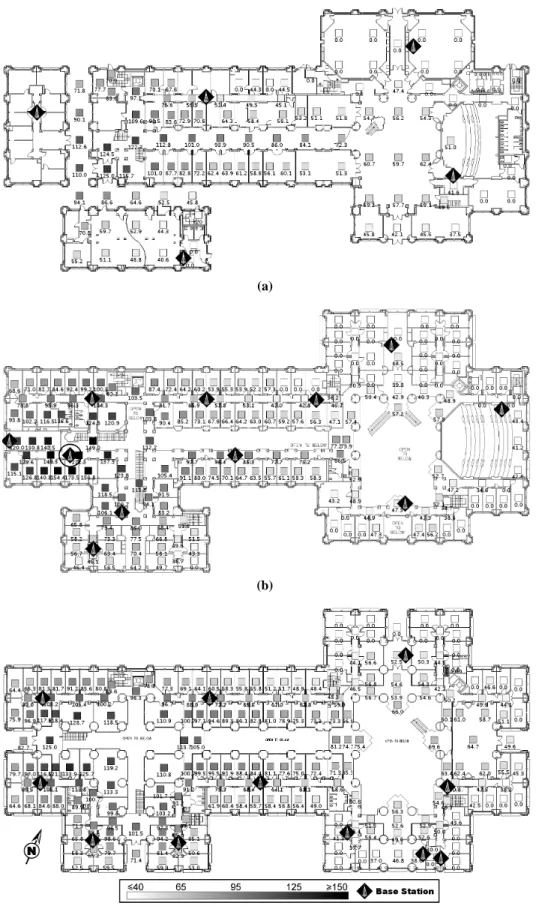
Figure 1: Sensor map within Duncan Hall for a base station located on the second floor. Base stations are represented as black diamonds with white antennas; the base station from which this sensor map was generated is circled. (a) is the first floor; (b) is the second floor; (c) is the third floor. Each shaded square represents a single training and testing cell. Darker squares indicate stronger readings.
(a)
(b)
(c)
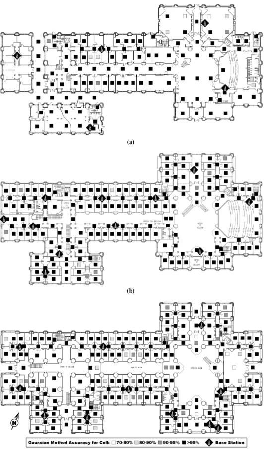
Figure 2: Map showing robustness of the Gaussian localization algorithm in Duncan Hall. (a) is the first floor; (b) is the second floor; (c) is the third floor. Each shaded square represents a single training and testing cell. The darkness of the square indicates the percent of trials for which the localizer indicated the correct location at that position.
2.3.2 Our building
We deployed our location-sensing system in Duncan Hall on the Rice University campus, a building which consists of three stories plus attic and basement utility spaces. Duncan Hall has over 200 offices, as well as several conference rooms, five classrooms, and an auditorium. The total area of the building is 12,558.4 square meters (135,178 square feet). Maps of the three floors of Duncan Hall are shown in Figures 1 and 2.
The most notable feature of our building is its complex geometry. The building has a large clerestory ceiling; the main hall on the east side of the building, the wide hallway connected to it, and staircases beginning at the hall and hallway are all open above. The hallways surrounding the atrium and the hallways passing over the wide hall-way on the second and third floors all contain balconies overlook-ing the first floor, and many of these are open to the clerestory ceil-ing above. In addition, all of the interior offices on the third floor are open above, and all but eleven of the interior offices have win-dows into the interior of the building.
2.3.3 Topology
We divided the building into 510 different cells on the topological map. This was done manually by placing cells on a floor plan of the building and took approximately one hour; for larger buildings, however, this process can be easily automated. Typically there is one cell per office. For large labs and lecture halls, however, the standard deviation of reported signal intensities would have been too high for localization to be usable. As a result, we assigned different cells to different regions of these rooms; these different cells were trained separately, but could be treated as a single cell for the purpose of localization. We also assigned cells to hallway segments. Figures 1 and 2 show how these training points are dis-tributed throughout the building.
Cell sizes varied over the building. The typical office size (and therefore, cell size) is approximately 2.7 by 4.9 meters (9 by 16 feet). The largest room trained as a single cell is approximately 6 by 6 meters (19.7 by 19.7 feet). Most hallways are 1.6 meters (5.3 feet) wide, and are partitioned into cells of segments approximately 5.7 meters (18.7 feet) long. We also trained cells for outdoor loca-tions, including third-floor balconies and a first-floor arcade.
To track agents as they move, we built a transition graph over the set of cells. This graph contains 1,159 edges (including self-transition edges), and the average out-degree is 3.55. It represents navigable paths in our building, encoding the fact that one cannot pass through walls except via doors, and one cannot switch floors except via a staircase.
2.3.4 Training
We obtained a master key for the entire building and collected at least 100 base station scans in each of the 510 cells. The person doing the training spent approximately 2.7 minutes in each cell. This person walked around slowly in order to cover the entire cell. The main goal in collecting the training data was to get a signal sample for each part of the cell; we did not concern ourselves with the relative position of the operator performing the training. Data collection took 28 man-hours overall; however, we collected many more scans than we needed to ensure that we would have indepen-dent data to experiment with. Had we only collected one minute of training data per office, the minimum we recommend for pro-duction use, training could have been accomplished in less than half the time. Keep in mind that data collection can be done con-currently; we collected our data using two operators, doubling our throughput. 0 2 4 6 8 10 12 70 75 80 85 90 95 100 Sample size Percent correct Gaussian Histogram
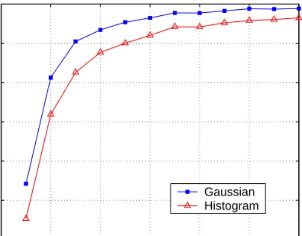
Figure 3: Bulk accuracy of localization methods after different numbers of observations.
We collected a total of 51,249 scans. On average, each scan con-tains a signal intensity reading from 14.86 of the 33 base stations. We observed intensity values ranging from 1 to 217; thus, we es-timate about 7.5 bits of usable information. When examining the intensity histograms, we found three fundamental types. Most of them were very close to Gaussian, so the Gaussian fit worked very well. Some were sparse, indicating that the base stations were al-most out of range; in these cases, the Gaussian fits had fairly large standard deviations. A few were bimodal; the estimated mean was in the middle, with a large standard deviation. Initially, we exper-imented with a bimodal weighted Gaussian fit, but our results for the single-mode estimator show that the improvements in accuracy would be marginal.
The sensor map of the entire building for a second-floor base sta-tion is shown in Figure 1; the base stasta-tion in quessta-tion is circled. As expected, signal intensity degrades fairly consistently as distance increases from the base station. There are several interesting phe-nomena of note. First of all, we can still reliably get a signal from the base station while outside or in a disconnected part of the build-ing (that is, through two exterior walls and windows). Second, the base station can be detected from across the building even on differ-ent floors. Finally, at long distances, some offices will see the base station while neighboring offices see nothing. This could be caused by multipath effects or by other variations in building geometry that result in favorable signal propagation.
2.4
Experimental results
2.4.1 Localization accuracy
The goal of this experiment was to determine the basic localiza-tion performance of our system using Gaussian-fit curves and to compare it with a system using the same training data but retain-ing the full histogram of signal intensity observations. We chose five scans at random for each of the 510 cells and removed them from the training set. The remaining scans were used to train our localizer. Then, for each cell, we used the scans we had removed from the training set as input to the localizer and attempted to lo-cate ourselves. We performed this experiment 100 times, removing different scans each time.
Figure 2 shows the test cells on the map of our building and the percentage of experimental trials in which the Gaussian method
0 20 40 60 80 100 0 10 20 30 40 50 60 70 80 90 100
Training Set Size
Percent correct
Gaussian Histogram
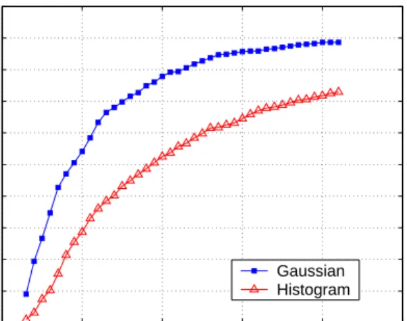
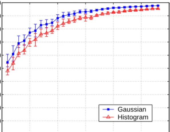
Figure 4: Training set size versus accuracy for the Gaussian and histogram methods.
returned the correct cell after five scans. In all cases, the Gaus-sian method determined the correct cell in at least 70% of trials; at all but a few locations, the localizer returned the correct cell in more than 90% of experimental trials. While the histogram method was likewise correct in at least 90% of trials at most lo-cations, there were several cells where the histogram method was correct in fewer than 50% of trials. Over all experimental trials, the Gaussian method was correct in over 97% of trials. The togram method was correct in over 95% of trials. While the his-togram method’s overall accuracy was comparable to the Gaus-sian method’s accuracy, the GausGaus-sian method has better behavior in pathological cases, typically returning a cell that is off-by-one from the correct location. This result is discussed in more detail in Section 3.1 and illustrated in Figure 8.
We wanted to explore the behavior of our system as we varied the number of observations from which the system infers location. The fewer observations required to infer a device’s location, the faster this inference can be generated; each additional observation adds an approximately 1.6 second delay in generating each location es-timate. We ran the same experiment as above, but chose from one to fifteen random scans for each cell to use for testing the localiza-tion. We performed this experiment 100 times for each cell. The results for one through twelve scans are shown in Figure 3; after twelve scans, the graphs show almost no further variance.
The results show that using one scan, both methods success-fully infer the location in over 70% of cases. 90% accuracy is achieved with at least two scans for the Gaussian method, and with at least three scans for the histogram method. It takes ap-proximately 1.6 seconds to perform a scan, so at that accuracy, we can localize the agent once every 3.2 seconds using the Gaussian method, and once every 4.8 seconds using the histogram method. Note that different hardware and driver combinations might be able to perform a scan faster, leading to shorter latencies between usable localization results.
2.4.2 Training set size
To evaluate the behavior of our localization system with smaller training sets, we chose training set sizes ranging from six to 90 samples per cell. When it takes 1.6 seconds to collect each sample, any reduction in the necessary training set size per cell will add up to a significant reduction in data collection labor over a large
0 20 40 60 80 100 0 10 20 30 40 50 60 70 80 90 100
Training Set Size
Percent of cells with >95% accuracy
Gaussian Histogram
Figure 5: Training set size versus percent of cells where 95% of trials returned the correct location.
building. As before, we chose five scans at random from our data to be our experimental scans. We then pruned the training set to the appropriate size by removing training points at random and fi-nally attempted to localize to each cell. We performed this test 100 times. The percentage of correct location estimates over all experi-mental trials for the Gaussian method versus the histogram method is shown in Figure 4.
The graph shows that both methods have good overall accuracy even at low training set sizes. However, the histogram method tends to require close to twice as large of a training set as the Gaussian method to attain a similar accuracy. The Gaussian method attains a 90% accuracy using only 16 training points; the histogram method requires 30 training points to attain this accuracy. Similarly, the his-togram method requires 84 training points to attain a 95% accuracy; the Gaussian method requires only 30 training points, correspond-ing to only 48 seconds in each office.
Accuracy also varies by location. Figure 5 graphs the percent-age of cells where at least 95% of experimental trials generated a location estimate corresponding to the actual location. This graph shows that the Gaussian method requires 24 elements in its training set to attain a 95% accuracy over 60% of the cells, 32 elements in its training set to attain a 95% accuracy over 70% of the cells, and 46 elements for a 95% accuracy of 80% of the cells. By contrast, the histogram method needs 52 elements to attain this accuracy over 60% of cells, and 74 elements in its training set to attain this ac-curacy over 70% of cells. We did not train with enough points for histogram to get 95% accuracy at 80% of cells. For other cut-off percentages (that is, other than 95%), we again observed that approximately half the number of training points are required to at-tain comparable levels of accuracy for the Gaussian method versus the histogram method.
Finally, we compared how many training points are required at individual cells before the localizer generates a correct location es-timate in at least 95% of experimental trials. Table 1 shows the number of cells for which an accuracy of 95% can be achieved with the histogram method and the Gaussian method as the number of training points increases; the caption provides detailed information on how to interpret the numbers in the table. At only two cells does the Gaussian method require more training data than the histogram method to attain a 95% accuracy. At over3/4 of the points, the
Method Histogram Histogram Histogram # of Training Points <30 30−60 >60 Gaussian 234 105 46 <30 Gaussian 2 17 68 30−60 Gaussian 0 0 67 >60
Table 1: Table showing number of cells at which the histogram and Gaussian methods first correctly localize to the cell in 95% of experimental trials as the training set size increases. The rows and columns are labeled with the number of scan records in the training set for each method we used. For instance, the 46 in the top right corner indicates that for 46 cells, the Gaussian method requires fewer than 30 training points to achieve 95% accuracy, and the histogram method requires over 60 training points to achieve this accuracy.
for most of the points, the histogram method requires at least 30 training points for 95% accuracy, and for over1/3of the points, it
requires over 60 training points. For most points, therefore, a 60-second training phase at each point (corresponding to a 37-element training set) is sufficient to localize most points to very good accu-racy using the Gaussian method.
2.4.3 Base station density
Localization accuracy is also influenced by the number N of base stations in the building. If N is reduced, less information is avail-able to the localizer, and thus the accuracy decreases. To quantify this effect, we performed another experiment in which we varied N by randomly removing some of the 33 base stations from our data set. In doing so, we ensured that at least one base station was still visible from each cell, and that at least 50 nonzero scans per cell remained. From the resulting data set, we took five random scans per cell and ran them through a localizer that was trained with the remaining scans.
The experiment was performed with both the Gaussian method and the Histogram method. For each value of N, we chose 20 ran-dom subsets of base stations and performed five trials for each sub-set. We report the overall fraction of trials in which the localizer was able to determine the correct cell, as well as the 20th and 80th percentiles.
Figure 6 shows our results. Even with only 17 instead of 33 base stations, the Gaussian method can determine the correct cell in over 90% of the trials. For lower values of N, the accuracy de-clines rapidly, while the fluctuations are significantly higher. This is because at lower densities, the exact placement of the base sta-tions starts to matter; also, the number of scans available to the localizer decreases because some of them contain only values for base stations that have been removed. If this were compensated by using an even larger data set, the results for lower densities would improve. However, in real-world wireless network deployments, it is reasonable to expect some redundancy of base station coverage to improve the quality and robustness of service.
3.
TIME-VARYING PHENOMENA
The localizer we have presented in the previous section assumes a static environment and a stationary agent. Neither assumption is realistic. The observed signal intensity distributions will often differ from the distributions estimated in the training phase due
5 10 15 20 25 30 35 0 10 20 30 40 50 60 70 80 90 100
Number of Base Stations
Percent correct
Gaussian Histogram
Figure 6: Impact of base station density on localization accu-racy. 18:000 22:00 02:00 06:00 10:00 14:00 18:00 32 64 96 128 160 192 224 256 Time
Average Signal Intensity
Figure 7: Signal intensity variation over a 24-hour period for three base stations measured from a laptop in a fixed location.
to a myriad of time-correlated phenomena. These phenomena in-clude environmental properties such as attenuation due to people in the building or building residents opening and closing their office doors. Likewise, transient interference can be caused by other elec-tronic devices including microwave ovens, Bluetooth devices, and cordless phones. Furthermore, a 2.4 GHz frequency corresponds to a 12.5cm wavelength, implying that multipath fading effects may be experienced even with small changes in the operator’s location. These dynamic environmental influences can cause the observed signal intensity to vary over both small and large timescales. The movement of the operator in the environment further complicates the task of maintaining an accurate position estimate.
3.1
Signal variations due to office traffic
Over the course of the day and throughout the night, many changes occur in the environment which affect the observed signal intensity. Each of these changes tend to be local and transient but since the nature and frequency of these events varies with the time of day, we expect that, on average, the signal intensity distribution changes globally on a larger timescale. In order to estimate the size of this
0 1 2 3 4 5 6 7 8 9 10 0 10 20 30 40 50 60 70 80 90 100
Distance to actual location (meters)
Percent of guesses
Gaussian (Calibrated) Histogram (Calibrated) Gaussian (Uncalibrated) Histogram (Uncalibrated)
Figure 8: Basic daytime performance for 27 cells. The results marked “calibrated” were obtained using the calibration tech-nique from Section 4.2.
effect, we collected scans at a fixed location (an office) over a 24-hour period. The resulting 52,900 scans were divided into groups of 100, and the signal intensities were averaged over each group. Figure 7 shows the result for three different base stations. There are noticeable variations during the day. At nighttime, some of them become less pronounced or more regular, while others disappear almost entirely.
Time-varying effects have severe implications on the accuracy of localization. To quantify these, we performed localization experi-ments in 27 different cells at around 11:00 AM, when there is rela-tively heavy traffic in the building, including students either in class or going to or from class. We collected approximately 30 scans in each cell and then ran each possible subset of five consecutive scans through the localizer; the probability vector was initialized with a uniform distribution each time. The results are presented in Figure 8. We observed mediocre results; using the Gaussian method, less than 70% of location estimates were correct, with the bulk of observed errors within 5.5 meters of the correct location. These results and techniques to improve them are discussed further in Section 4.
3.2
Tracking
Another time varying phenomenon we examined is the movement of the agent. Markov localization works well as a single-shot local-ization algorithm or for a stationary agent; however, for a moving agent, the prior position estimate will hamper correct localization. A simplistic solution can be obtained by resetting the distributionπ to a uniform distribution over all states between each burst of obser-vations. A more elegant and effective solution is to update the state estimate between each set of observations using a Markov chain that encodes assumptions about how the agent can move from state to state.
Suppose at time t, the state estimate isπt. Between time t and
t+1, the agent moves in some unknown way. At time t+1, the observations o1,...,okare received. The state estimate at time t+1
is computed as follows: πt+1 i = ∏k j=1P(oj|si)πti+ η , B E H J M I K L G F A C D
Figure 9: The floor plan for part of Duncan Hall and the corre-sponding Markov chain.
where
πt+= Aπt.
As before,ηis a normalizer that ensuresπt+1is a probability
vec-tor. The probability matrix A encodes the Markov chain, which can be thought of as a finite state machine (Figure 9). States represent cells, and an edge from state sito state sjindicates that cell j can be
reached directly from cell i. Also, each edge is assigned a transition probability Ai,j. In our implementation, we gave a fixed probability
to the self-edge at each state and distributed the remaining proba-bility evenly across its outgoing edges.
3.3
Tracking experiments
We wanted to evaluate the effectiveness of Markov chains when tracking a moving agent. First, we randomly chose four way-points in our building. Then we simulated a person following the short-est path between these way-points; the simulated agent remained at each way-point between 10 and 15 seconds, and moved with a constant speed between 0 and 4.5 meters per second (between 0 and 10.1 miles per hour) from one way-point to the next. Every 1.6 seconds, we chose a random scan from the closest cell to the agent’s simulated location.
This timing simulates the agent performing back-to-back base station scans. The agent would not be able to communicate over the network while tracking. As a compromise, the agent could in-terleave scans and communication, e.g. by using the interface for data traffic for 1.6 seconds in between each 1.6-second scan. In
0 0.5 1 1.5 2 2.5 3 3.5 4 4.5 50 55 60 65 70 75 80 85 90 95 100 Walking speed (m/s) Percent correct With Adjacent With Lag Correct
Figure 10: Accuracy of dynamic tracking as a simulated per-son walks around our test area. Correct is the overall percent of correct location estimates. Lag is the overall percent of lo-cation estimates that match either the current or the previous cell. With Adjacent is the overall percent of location estimates within one location cell in our topological model.
this experiment, a person using such a system would appear to be moving at twice her actual speed.
These scans were then run, in order, through the localizer. We also passed the location estimate through a hidden Markov model of the agent’s movement through the environment. The initial prob-abilities for the hidden Markov model were set to 1.0 for the correct cell and to 0.0 for all other cells. We performed this experiment 250 times for each speed. The results are shown in Figure 10.
The Correct result is the overall percent of correct location es-timates. This value decreases slowly until a velocity of 4 meters per second (8.9 mph), and even at this speed, the localizer has an accuracy of 71%. The Lag result is the overall percent of location estimates that match either the current or the previous cell. By this metric, our method experienced a similar drop-off of accuracy at 4 m/s. The localizer had an accuracy of over 79% at this speed. Finally, the With Adjacent result is the overall percent of location estimates within one location cell in our topological model; by this metric, the localizer had an accuracy of 86% at 4 m/s.
This demonstrates that our localization method, when coupled with a hidden Markov model of motion, can accurately track even a fast-moving target. As expected, the overall accuracy is lower than for static localization. Even at a slow walking pace, only four scans might be registered before the agent enters a new cell, so it is unsurprising that localization accuracy is lower for moving than for stationary agents. The hidden Markov model helps the sys-tem by, in effect, anticipating this movement and rejecting unlikely measurements when they would otherwise predict impossible tran-sitions. Also note that different hardware and driver combinations might be able to complete a scan faster than the 1.6 seconds we experienced; this would greatly improve our results.
Another interesting phenomenon we were concerned about was that the tracker might get “stuck” in an office adjacent to the agent’s current location. Because there were no direct edges connecting ad-joining offices, the tracker might not make the transition. Although we considered adding “phantom” edges to the transition matrix A to account for this behavior, the tracker would, in practice, follow
first the edge from the adjacent office to the hallway, and from there to the correct office, thus correcting for such errors automatically.
3.4
Miscellaneous effects
To illustrate the impact of time-varying phenomena on tracking per-formance, we report some insights from our practical experience with the system. One of the authors was using the tracker over a normal office day, during which he attended a lecture and a presen-tation, worked at his desk, and walked from office to office. The overall performance was very satisfactory; the estimated location occasionally jumped to an adjacent cell, but generally matched the true location well.
The presentation, which was held in a conference room full of students, turned out to be a worst-case scenario. The signal was not only heavily attenuated, but also changed over time, for example when a fellow student leaned over and thus moved closer to the antenna. This caused the estimated location to jump between the three different cells in the conference room, and occasionally to the cell right outside the door. Similar effects were observed when the author met other students in the hallways and was asked to explain the experiment. As soon as the other person moved close to the antenna in order to watch the location estimate, the estimate jumped to an adjacent office.
4.
CALIBRATION
The sensor maps built by our method can only be guaranteed to work for localization if they are used in the same environment as during the training period. However, as shown in the previous sec-tion, the environment can change significantly over the course of the day. Moreover, the signal intensity values reported by the hard-ware depend on various factors, including the chipset and the an-tenna, and can vary considerably between different 802.11 imple-mentations. Therefore, a method is needed to adapt the sensor map to the environment in which it is to be used.
Fortunately, we observed that the effect of environmental changes, including both time-varying effects and different hard-ware, can be closely approximated by a linear relationship. Thus, the sensor map can be adapted to a new environment simply by learning two parameters. This process, which we refer to as
cal-ibration, should require little or no user intervention; ideally, it
would be performed in the background, thus enabling the localizer to work “out of the box.”
In this section, we first describe the model we use for calibra-tion and give several examples of different configuracalibra-tions and the corresponding parameters. Then we present three different cali-bration methods, spanning the range from completely manual to completely autonomous.
4.1
Model
The calibration problem can be formulated as follows: Given a sen-sor map and an 802.11 device in a certain environment, find a
cali-bration function c that maps an observed signal intensity value i to
the value c(i)that would have been reported by the device that was used to generate the sensor map. If c is known, c(i)can be given as an input to the localizer, and the original sensor map can be used unmodified.
As Tao et al. [48] first observed, there is a linear relation between transmission power level and received signal strength as reported by 802.11 hardware. In our experiments, we discovered that the effects of hardware variation and some time-varying phenomena appear to be linear as well. That is, the calibration function can be
Chipset Relation ACX100 c(i) =i
Prism c(i) =0.85·i−43.5 Atheros c(i) =2.77·i−409.5
Table 2: Linear relationships between several different 802.11 cards and the ACX100 card we used in training. i is the value reported by the hardware, and c(i)is the equivalent value that would be reported by the ACX100, and that can be input into the localization system to accurately determine the device’s lo-cation.
closely approximated by the linear relationship
c(i) =c1·i−c2.
Thus, it is sufficient to learn the parameters c1and c2in order to
adapt a given sensor map to a new environment. This can be accom-plished in various ways; for example, one can collect some mea-surements at well-known locations and compute the least-squares fit between the observed values and the corresponding values from the sensor map.
Using this method, we found the parameters for a number of different cards. These are listed in Table 2. The ACX100 is the card we used for training, so its calibration function is the identity function. Prism is a Linksys WPC11 PCMCIA card based on the Intersil Prism2 chipset. Atheros is a Mini PCI card with an Atheros chipset and using the IBM Thinkpad T40p’s built-in antenna.
Figure 11 shows the effects of calibration for the Atheros chipset. This ‘unadjusted’ graph was generated using pairs(iR,iM)of
inten-sity values, where iR is the reference value from the sensor map
for a certain cell and base station, and iM is the corresponding
value measured with the Atheros card. The ‘adjusted’ graph shows
(iR,c(iM)), clearly indicating that after calibration, the two values
are almost identical.
Note that the signal intensities reported by the Atheros chipset were 8-bit values as in the ACX100 case, but we observed only values between 163 and 224, so there are only 5.9 bits of usable information.
That is not to say that the difference in signal strength reporting between any two cards is always a linear relation. In particular, dif-ferent cards may use difdif-ferent techniques to actually measure the signal strength. As Steger et al. [47] demonstrated, different cards behave differently in the face of varying signal conditions. In addi-tion, as indicated by our results, the mapping from the actual signal strength to the number returned by the hardware is arbitrary, will vary from one chipset to another, and need not be linear. However, in all the cards we tested, the signal strength readings were linear relations of one another.
4.2
Manual calibration
As mentioned earlier, the parameters of the calibration function can be found by computing a linear fit for a set of measured signal in-tensities and the corresponding values from the sensor map, e.g. by applying the least-squares method. First, we must collect enough value pairs to perform this calculation. In our prototype implemen-tation, this is done by moving the device to several different cells. In each cell, the user presses the ‘calibrate’ button, prompting the device to collect a few scans, and then indicates the current cell on a floor plan of the building. Since in Duncan Hall, each cell contributes value pairs for 14.86 base stations on average, a small number of cells (three to five) was usually sufficient.
0 32 64 96 128 160 192 224 256 0 32 64 96 128 160 192 224 256
Signal intensity (reference) Signal intensity (new card) Unadjusted
Adjusted Ideal
Figure 11: Effect of calibration on the signal strength values reported by the Atheros chipset. The intensity values shown are averages over at least five samples.
0 32 64 96 128 160 192 224 256 0 32 64 96 128 160 192 224 256
Signal intensity (reference)
Signal intensity (observed) Unadjusted Adjusted Ideal
Figure 12: Average signal intensity values, before and after re-calibration for time-varying effects.
Figure 12 shows an example result from such a calibration. In this case, the 802.11 hardware was the same as during the training period, but the measurements were taken at daytime during heavy office traffic. Clearly, both the constant offset and the linear factor changed. Yet, after calibration, the signal intensity values corre-spond almost exactly to the ones from the training phase.
In order to quantify the effect of calibration for time-varying ef-fects, we ran the localization with and without performing calibra-tion. The result is shown in Figure 8. Without calibration, the results are mediocre: less than 70% of location estimates are cor-rect, and 90% of estimates are within 5.5 meters for the Gaussian method. After calibration, results are greatly improved: 88% of location estimates are correct, and 90% are within 3 meters. This experiment suggests an important conclusion: that a single linear-fit captures most of the deviation induced by slow timescale phe-nomena. In other words, the signal intensity shifts due to slow time-varying effects seem to be homogeneous on average across various locations. Qualitatively, we have observed that running lo-calization without tracking, during the day, is a bit noisy, lags a
bit, and is prone to localizing into the room adjacent to the user. Once we run the calibration in three or four cells, the localization is extremely stable and very rarely makes mistakes.
4.3
Quasi-automatic calibration
Manual calibration is clearly effective, but has the disadvantage of requiring the user to specify the current cell. Surprisingly, however, calibration can be performed without this information and using
only a set of scans from several different – but unknown – cells.
Our second calibration method takes advantage of the fact that the observation space is both sparse and non-linear, so there is al-most never a linear mapping between observations from different cells. Hence, when an incorrect calibration function is used, the calibrated intensity values do not match any reference values from the sensor map, and the confidence valueηproduced by Markov localization (see Section 2.2.1) is low for all cells; it is high only if
both the calibration function and the cell are correct. Therefore, the
parameters c1and c2can be learned by attempting Markov
local-ization and by choosing values such that the confidenceηis maxi-mized.
4.4
Automatic calibration
Although the quasi-automatic method involves less user interaction than the manual method, it still requires the user to press a ‘cali-brate’ button from time to time. However, in order to obtain op-timum performance, the user will have to recalibrate several times over the course of the day, which is cumbersome and, in the case of manual calibration, requires a certain familiarity with the build-ing. It would be clearly preferable to have an entirely hands-off solution.
Toward this end, we have been investigating the problem of run-ning localization, tracking, and calibration simultaneously. Our ini-tial results are promising but do not yet match the results we have seen with supervised calibration for online localization and track-ing. The basic technique we have been considering uses a history of recent observations as a training sample to construct an estimate of the calibration parameters that are then used to process future data. This algorithm runs in parallel with the localization process. We use an expectation-maximization algorithm (E-M) [52] that com-putes a fixed-point, iterating between inferring a sequence of lo-cation estimates from the history and then choosing c1,c2to
maxi-mize the probability of these estimates occurring. The observations and estimates are stored in a sliding window of between 10 and 45 seconds.
Our current implementation of simultaneous localization and calibration seems about as good as supervised calibration for static localization problems. In the tracking implementation, we have ob-served that the tracker is a bit sluggish and prone to place the user in adjacent rooms. Also, it seems to occasionally get stuck with a bad hypothesis that stays until the sliding window fills with new data. If the size of the sliding window is decreased then the tracker lags.
Another possible approach that we believe may be attractive is a Monte Carlo (particle filter) approach [18, 53] that maintains a set of c1,c2 hypotheses and gathers data to determine which
hypoth-esis should be used. Where our current approach only maintains one hypothesis at a time, this approach would simultaneously try a large number of hypotheses, preventing the system from getting stuck with a local maximum and thereby missing globally optimal settings. In this framework, the confidence values from the local-izer (η) could be used to discriminate between two hypotheses. Our
experiments and data analysis suggest that solving the problem of making a simultaneous localizer and calibrator is tractable.
5.
DISCUSSION
5.1
Why a Gaussian fit?
Our most striking departure from previous work is that the most successful systems in the literature have used the entire signal in-tensity histogram. On the other hand, we have chosen to fit the sensor map data to Gaussian distributions. We chose this course for several reasons.
First, fitting the data to a Gaussian only requires storing two numbers for each base station and cell. Keeping the entire his-togram requires at least 30 times as much storage. This reduction increases the speed and reduces the memory requirements for local-ization, making it more suitable for low-power embedded devices that may not have the resources of a modern laptop computer.
Furthermore, fitting to a Gaussian also provides some robust-ness benefits to our system. The Gaussian method tends to provide roughly the same accuracy of localizations for half the training ef-fort (see Section 2.4.2). One reason for this is that if the entire histogram is used, the training might capture minor modes that are a result of time varying phenomena and might miss other minor modes not present in the training set. These minor modes will be covered by the normal distribution curve to which the data is fit in the Gaussian method. Also, previous histogram-based systems re-quired taking as many as 500 scans to train each point. This would make it impractical to build a sensor map as large as the one we built without a significantly longer training time.
5.2
Choosing a training set size
Although most of our localization results are based on training sets with 90 elements, we determined that for our building, taking a 60-second training set (around 37 elements) was adequate for accurate localization in most of our building (see Section 2.4.2). The point of diminishing returns, in terms of accurately capturing the sensor map, seems to begin around 35 samples per point (see Figure 4). Of course this is a minimum; having additional training data can only help.
The optimal number of training points depends on a number of factors, including building geometry, base station density, and building usage. Although Duncan Hall has unusual geometry, the base station density is high; there are rarely fewer than five base sta-tions in range, even in the corners of the building. Buildings with fewer base stations, lower base station density, or more opaque con-struction materials, would likely need larger training sets.
Buildings with interesting geometry, such as large open areas, tend to dilute differences in signal intensity, and require more train-ing data. As the sensor map in Figure 1 shows, hallways tend to channel signals such that signal intensity drops at a regular rate going down a hallway. Large open areas tend to disperse signal, leading to much less distinction among cells.
To adequately measure signal maps in other buildings, experi-mentation may be necessary to determine the ideal set size. For our own building, we started by first collecting training data in a small region of the building. By observing the mean and standard deviations of this data, we could estimate how many samples were necessary for the system to converge. In our own case, we ob-served that, with 25 scans, the variation of the mean dropped below 2. For experimental purposes, we captured significantly more than 25 scans per cell to help verify our results.
It would be possible to encode the above technique into the train-ing system. When the mean and standard deviation stabilize to
within a specified threshold, we can conclude that we have col-lected enough training data to accurately describe a cell. This check could be run in real-time.
5.3
Changes to the infrastructure
In this paper, we implicitly assumed that the sensor map accurately reflects the signal intensities throughout the building. However, this is only true as long as there are no fundamental changes in the en-vironment, such as base station failures or major reconfigurations. While changes of this type are infrequent in practice, they may af-fect localization accuracy where they do occur.
If an individual base station fails, it does not respond to probe re-quests any more and thus changes the observations made from the surrounding cells. However, because our method only uses posi-tive observations, i.e., probe responses actually received, the only effect this has on the localizer is that there is less information avail-able, reducing accuracy and convergence speed. As long as enough other base stations are in range, the effect should be small (see Sec-tion 2.4.3).
Moving an existing base station requires the cells surrounding the old and the new position to be re-trained. However, since base stations are typically wall-mounted and require power and a net-work connection, they cannot be moved easily, so changes of this type should be very rare.
The appearance of transient base stations does not affect local-ization because the localizer can easily determine the set of accept-able stations from the signal map and ignore unknown stations. If a permanent station is added after the training phase, it can be used to improve accuracy by re-training the cells from which it is visible.
Some base stations choose their channels dynamically; thus, a major failure such as a power outage may cause the channel as-signment to change. This actually happened once during our ex-periments, when a maintenance event required the entire building to be taken off-line. Although the base stations operated on differ-ent channels afterwards, we did not observe a significant change in accuracy.
5.4
Passive localization
Passive localization refers to localization in which the mobile de-vice being localized is a passive participant in the localization pro-cess. While the device must be transmitting data to be tracked, it is not explicitly performing any part of the localization algorithm, and need not be aware that it is being tracked. Since signal propagation is a reversible operation, the same sensor map data should, after calibration, allow someone with access to enough receivers to track any transmitting device. While we’ve performed some experiments that tend to validate this, more experimentation is in order.
The most obvious application of passive localization is for locat-ing an intruder on an 802.11 wireless network. Tao et al. [48] per-formed a study of this issue. Two problems they overcame were dif-ferences in hardware and difdif-ferences in transmission power. Since both of these were fixed by mapping received signal intensity to the training set via a linear relation, the calibration technique we discuss in Section 4 should allow us to account for both of these variations. A promising avenue of future work is applying simulta-neous localization and calibration (see Section 4.4) to automatically account for variations in hardware, movement, and transmission power manipulation on the part of the intruder.
Finally, more ambitious intruders might attack in coalitions, jointly transmitting packets using the same hardware address. This would make the attacker appear to be jumping all over the map. We
believe clustering algorithms may be able to adequately determine the number of attackers and separately localize each one.
There are of course privacy implications to being able to track any arbitrary device on an 802.11 network. Anyone who has phys-ical access to a building can deploy an ad hoc network of snoopers and track every device in the building, with or without the approval of the building’s management. The only solution is to realize that, by transmitting a packet on an 802.11 network, a mobile agent is effectively revealing its location to motivated adversaries.
6.
CONCLUSION
In this paper, we presented a practical robust scheme for local-ization over the entirety of an 802.11 network deployed within a multi-story office building. We have shown that the use of a topo-logical model can dramatically reduce the time required to train the localizer, while the resulting accuracy is still sufficient for many location-aware applications. We used a Gaussian fit sensor model, which is more robust and requires less training compared to sensor models that use the full histogram of signal strengths. Finally we developed a technique by which the training data can be adapted for use with totally different receiver hardware, and under different conditions than during the training phase.
To evaluate our localization technique, we have developed a methodology which makes use of excess training data to determine raw localization performance. We deployed our system in a large office building on the Rice University campus. In our experiments, we experienced both good overall performance and excellent ro-bustness; in the rare event that an incorrect position estimate was generated, it was almost always to an adjacent cell. We also dis-covered how different variables, including training set size, sample size, base station density, and time of day affect localization accu-racy.
Our system is ready to be made available right now in our office building for people who want to use location-aware applications on top of it, and it could be made available in the near future for deployment (after a brief training phase) in any building with an 802.11 network installed.
7.
ACKNOWLEDGEMENTS
This paper has benefited considerably from the comments of the anonymous MobiCom reviewers and our shepherds, Per Gunning-berg and Farooq Anjum. We would like to thank Kostas Bekris, Guillaume Marceau, and Ping Tao for contributions to earlier versions of this work. In addition, thanks to Joseph Cavallaro, Ashutosh Sabharwal, and Patrick Frantz for their insight into how wireless network cards measure signal strength. Finally, thanks to all the residents of Duncan Hall for their cooperation in our exper-iment, and the department chair, Keith Cooper, for trusting us with his master key.
Andreas Haeberlen is partly supported by NSF ANI-0338856 and by a fellowship from Rice University. Andrew M. Ladd is partly supported by NSF 0308237 and a FCAR Fellowship. Algis Rudys and Dan S. Wallach are supported by generous gifts from Microsoft and Schlumberger. Lydia E. Kavraki is partly supported by NSF 0308237 and a Sloan Fellowship.
8.
REFERENCES
[1] G. Abowd, K. Lyons, and K. Scott. The Rhino project, Aug. 1998. http://www.cc.gatech.edu/fce/uvid/