New Procedures of Estimating Proportion and Sensitivity Using Randomized Response in a Dichotomous Finite Population

Volume 15 | Issue 1 Article 32

5-1-2016

New Procedures of Estimating Proportion and

Sensitivity Using Randomized Response in a

Dichotomous Finite Population

Tanveer A. Tarray

School of Studies in Statistics, Vikram University Ujjain - M.P. - India., [email protected]

Housila P. Singh

School of Studies in Statistics, Vikram University Ujjain, M.P., India, [email protected]

Follow this and additional works at:http://digitalcommons.wayne.edu/jmasm

Part of theApplied Statistics Commons,Social and Behavioral Sciences Commons, and the

Statistical Theory Commons

Recommended Citation

Tarray, Tanveer A. and Singh, Housila P. (2016) "New Procedures of Estimating Proportion and Sensitivity Using Randomized Response in a Dichotomous Finite Population,"Journal of Modern Applied Statistical Methods: Vol. 15 : Iss. 1 , Article 32. DOI: 10.22237/jmasm/1462077060

Cover Page Footnote

The authors are thankful to the Editor – in- Chief, and to the anonymous learned referee for his valuable suggestions regarding improvement of the paper.

Dr. Tarray is affiliated with the Department of Computer Science and Engineering. Email him at: [email protected]. Dr. Singh is affiliated with the School of Studies in Statistics.

New Procedures of Estimating Proportion

and Sensitivity Using Randomized Response

in a Dichotomous Finite Population

Tanveer A. Tarray Vikram University Ujjain, M. P., India Housila P. Singh Vikram University Ujjain, M. P., India

The problem of estimating the population proportion possessing a sensitive attribute using simple random sampling with replacement (SRSWR) is advocated. Two new procedures are proposed. The suggested models are more efficient than the Huang (2004) randomized response technique under some realistic conditions. Numerical and graphic illustrations are given.

Keywords: Randomized response technique, direct response, estimation of proportion, privacy of respondents, sensitive characteristics

Introduction

Socioeconomic investigations often relate to certain personal features that people desire to hide from others in comprehensive inquiries, detailed questionnaires include numerous items. Direct questioning of respondents about them is likely to result either in non–response or in a deliberately incorrect answer. Social stigma and fear of reprisals often lead respondents to give biased, misleading, or even erroneous responses when approached with a direct response (DR) survey method. Even for the reason of merely being unwilling to reveal secrets to strangers, many individuals attempt to avoid certain questions put to them by interviewers.

Consider a dichotomous population in which every person belongs to either a sensitive group A or to the non–sensitive complement Ac_{. The aim is to estimate π,}

the population proportion of individuals who are members of A. To do so, a simple random sample of size n is drawn from the population with replacement. Let T be the probability that the respondents belong to A report the truth. The respondents

belonging to the non–sensitive group Ac _{have no reason to tell a lie. For a DR survey}

of size n, the interviewee is asked if they are a member of A. Then we have a direct estimator 1 ˆ n i i D X n



_



 ₍₁₎

with mean square error (MSE) given by

 

_ˆ



1



2





2

MSE _D D D 1 T n







  



 (2)

where Xi = 1(0) if the ith _{interviewee responds Yes (No) and θD = πT.}

To procure reliable sample data for the population proportion of the respondents belonging to the sensitive group A, Warner (1965) proposed an ingenious procedure called Warner’s randomized response technique. This pioneering work led to modification and developments in several directions; for instance, see Fox and Tracy (1986), Mangat and Singh (1990), Mangat (1994), Mahmood, Singh, and Horn (1998), Chua and Tsui (2000), Sing, Singh, and

Mangat (2000), Chang and Huang (2001), Huang (2004), Chang, Wang, and Huang

(2004a, b) and Singh and Tarray (2012, 2013a, b, c, 2014a, b, c, d, e).

Huang (2004) pointed out there are many variants of the randomized response technique in the literature, but most do not dwell on the fundamental question: whether or not the issues considered in the survey should be regarded as sensitive, meaning that there is a need for a randomized response procedure rather than a direct response procedure. In general, the probability T is a measure instrument of the sensitivity (see Huang, 2004). It has a primary use in appraising the efficiency of different survey plans. One may use a simple formula for ascertaining whether a randomized response technique is beneficial in efficiency relative to a DR scheme. However, the probability T is unknown in actual practice. To overcome such a difficulty, Chang and Huang (2001), Huang (2004), and Chang et al. (2004a) have suggested alternative survey strategies which make it possible to estimate the unknown parameters π and T simultaneously. Two alternatives to Huang’s (2004)

A Brief Review of Randomized Response Models

Warner’s Models

In order to improve respondent cooperation and to encourage honest response,

Warner (1965) proposed the following procedure, known as a randomized response

technique (RRT). Instead of a DR procedure, a randomization device is used to gather sample information consisting of one of two statements:

(i) “I am a member of group A”

(ii) “I am not a member of group A”

with probabilities P and (1 - P) respectively. Following this device, the respondent selects a statement unobserved by the interviewer, and then simply gives a “Yes”

or “No” answer in a random sample of n respondents. By the method of moments,

Warner obtained an unbiased estimator of the population proportion π possessing

the sensitive attribute A:



1



1 ˆ , 2 1 2 W Y P P P



     ,

where Yi = 1(0) if the ith _{respond answers Yes (No) and}

1 1 2 n i i Y 



_ y . The variance of



ˆ_W is given by

 





















2 2 1 ˆ V , 2 1 1 1 2 1 W W W n P P P n n P











        , (3) where θW = πP + (1 – π)(1 – P). Singh Models

Singh (1993) developed two randomized response techniques named RRT1 and

RRT1: In this procedure, each interviewee in A with replacement simple random sample of size n is provided with one randomized response device. It consists of the statement “I belong to the sensitive group” with known probability P, exactly the same probability as used by Warner (1965) and the statement “Yes”

with probability (1 – P). The interviewee is instructed to use the device and report “Yes” or “No” for the random outcome of the sensitive statement according to his/her actual status. Otherwise, he is simply to report the “Yes” statement observed on the randomized response device. The whole procedure is completed by the respondent, unobserved by the interviewer. Then θ1, the probability of a “Yes”

answer in the population, is





1 1

S P P







  .

An unbiased estimator of π due to Singh (1993) is given by





1 1 ˆ ₁ ˆ S S P P





   ,

where



ˆ_S1 is the proportion of “Yes” answers in the sample of size n. The variance of the estimator



ˆ_S1 is given by

 

1



 





1 1 1 ˆ V _S P n nP          . (4)

RRT2: This procedure is exactly like RRT1 except for a change in probabilities on the randomized response device, i.e., the probabilities for the “sensitive” statement and “Yes” statement have been interchanged. The probability of a “Yes” response is then



2



2 ˆ ˆ 1 S S P P





   ,

 

2





_



_



1 1 ˆ V 1 S P n n P          . (5)

Huang (2004) showed that his procedure resulted in better performance as

compared to the Warner (1965) and Chang and Huang (2001) procedures.

Huang Model

In this procedure, a simple random sample of size n is drawn with replacement from a finite population. The sampled individuals are required to reply to a direct query as to whether or not they belong to A. When answering “No”, the respondent is provided with a randomization device consisting of two statements:

(i) “I am a member of A”

(ii) “I am not a member of A”

with probabilities P and (1 – P), respectively.

It is assumed that the respondents belonging to A give totally honest responses under the randomized response procedure, but with probability T following the usual direct response procedure. The probability of a “Yes” response in the direct response procedure is given by

1 T

 

 , and in the randomized response procedure by



 



 







2 P 1 T 1 P 1 2P 1 P T 1 P







   



 







  .

Huang (2004) suggested the following estimators of π and T respectively as









1 2 ˆ ˆ ₁ ˆ 2 1 H P P P           and









1 1 2 ˆ 2 1 ˆ ˆ ˆ ₁ H P T P P       _{  }    ,

where ˆ_j, the observed proportion of “Yes” answers, is the binomial random variable with parameters n and θj, j = 1, 2. Huang (2004) obtained the variance of

ˆ_H



as

 















2 1 1 1 ˆ V 2 1 H P P T n _{n P}









      (6)

and the MSE of the estimator Tˆ_H, up to terms of order O(n-1_{), as}

 







_

 

2

_



2 2 1 1 1 ˆ MSE 2 1 H T T P P T T T n n P          (7)

Proposed Procedures

HRRT1

In this procedure, a simple random sample of size n is drawn with replacement from a finite population. The sampled individuals are instructed to answer a direct query as to whether or not he/she belongs A. When answering “No”, the respondent is provided with a randomization device. It consists of the statement “I belong to the sensitive group” with known probability P, exactly the same probability as used by Warner (1965), and the statement “Yes” with probability (1 – P) (Singh 1993, p.

68). The interviewee is instructed to use the device and report “Yes” or “No” for

the random outcome of the sensitive statement according to his/her actual status. Otherwise, they are simply to report the “Yes” statement observed on the randomized response device. The whole procedure is completed by the respondent, unobserved by the interviewer. Then θt1, the probability of a "Yes" answer in the

population, is 1 1 t t T T









  

And, adopting the randomized response procedure, the respondent gives totally honest responses under the randomized response procedure by



 



1 2





1 1 1 1 t t t P P P T P P











    



     .

Thus the proposed estimators of π and T are given by





1 1 1 ˆ ˆ ₁ ˆ t t a P P P







     and





1 1 1 2 ˆ ˆ ˆ ˆ ₁ t t t P T P P            ,

respectively, where ˆtj, the observed proportion of “Yes” answers, is the binomial random variable with parameters n and θtj, j = 1, 2. The principal properties of the estimator



ˆ_a1 are outlined in the following theorem:

Theorem 1. The estimator



ˆ_a1 is unbiased with the variance given by

 

1



 





1 1 1 ˆ V _a P T n nP            (8)

Proof. The unbiasedness follows from E

 



ˆ_tj 



_tj, j1, 2. The variance of the estimator



ˆ_a1 can be obtained as follows:

 

   

































 





2 1 2 1 2 1 2 2 1 1 2 2 1 2 2 2 2 2 2 1 2 1 2 1 2 2 2 2 1 2 1 2 2 2 2 1 _{ˆ ˆ ˆ ˆ} ˆ V V V 2 cov , 1 1 2 1 1 2 1 1 1 1 1 1 1 1 1 a t t t t t t t t t t t t t t t t t t t t P P P P P P n n n P P P nP P P nP P P P T nP P T n P                                 _   _      _   _      _     _    _    _    _      _       _   _  

Hence the theorem.

An unbiased estimator of the variance V

 



ˆa1 can easily be obtained, which

is given as follows:

Theorem 2. The unbiased estimator of V

 



ˆa1 is given by

 

₁



₁

 



_



_

1 1



1 ˆ ˆ 1 1 ˆ 1 ˆ ˆ V 1 1 a a a a a P n n P              (9)

To form an idea about the sampling fluctuation of the direct estimator



ˆ_D from the sample itself, one has to develop an estimator of MSE

 



ˆ_D . In fact, with the help of the proposed procedure, one can find an unbiased estimator of the MSE of



ˆ_a1, which is presented in the following theorem:

 





_

_





 





_

_

 

2 1 1 1 1 1 2 1 1 1 1 2 1 ˆ ₁ 2 ˆ _ˆ ˆ _{ˆ ˆ} ˆ _ˆ MSE 1 V 1 ˆ 2 ˆ _ˆ ˆ ˆ _Vˆ _ˆ 1 t D t a a a t t a t t a P n p P P n P                   _   _         _   _ 

Proof. The proof is straightforward and is therefore omitted.

To obtain the bias and MSE of the estimator ˆT , we write d₁P



ˆ₁ and





2 ˆ1 ˆ2 1

d _P

 

  P _, and it follows that E(d1) = PπT and E(d2) = πP. The

estimator ˆT can then be represented as Tˆd d_{1 2}, and we have T = E(d1)/ E(d2).

Furthermore, we define the following quantities:

 

 

1 1 1 1 E E d d e d   and

 

 

2 2 2 2 E E d d e d   ,

assuming that |e1| < 1 so that the function (1 + e2)-1 can be validly expanded as a

power series. It can be easily proved that

 



 







 









 





1 1 1 1 1 2 1 2 2 2 1 1 2 1 1 2 2 1 2 2 2 2 2 1 1 1 2 1 2 2 1 1 1 E , 1 1 2 E , 1 E t t t t t t t t t t t t t t t t t e n n n T P P e nP P e e nP T                                  













 

1 1 1 2 1 2 1 1 2 1 1 2 1 2 1 1 2 1 ˆ (1 ) 1 (1 ) 1 (1 ) ˆ _{( ) o} t t t P P e T T T P e P T e e T P T e e T T T T e e n



 







                    

We then state the following theorem:

Theorem 4. The MSE of the estimator Tˆ1, up to terms of order o(n−1), is given

by

 



 

 

2



1 2 1 1 1 ˆ MSE T T T P T T n nP           (10) Proof. Consider

  



 

 

 



































2 1 1 2 2 2 1 1 2 2 1 1 1 2 1 1 2 _{2 2 2 2} 2 1 1 2 2 1 2 2 2 2 2 1 1 1 2 2 2 2 2 2 2 2 2 2 1 2 2 2 ˆ ˆ MSE E E 2 E E 2 1 1 1 1 2 1 1 2 1 1 1 t t t t t t t t t t t t t t t t t t t t T T T T e e e e P T _{T P T} n _{P P} P T T T n T PT P P T T T n P                               _   _   _   _         _{   }        _{   }             













_

_

2 1 2 2 2 2 2 2 1 1 1 1 1 1 t P T t T T P T T T T P T n P       _{   }              _  _   _  



 

 

2



2 1 1 1 T T P T T n nP          

Hence the theorem.

HRRT2

In this proposed method, a simple random sample of size n is drawn with replacement from a finite population. The sampled individuals are required to reply a direct query as to whether or not they belong to A. When answering “No”, the respondent is provided with a randomization device consisting of the statement “I belong to the sensitive group” with known probability (1 – P), exactly the same probability as used by Warner (1965), and the statement “Yes” with probability P (Singh 1993, p. 68). The interviewee is instructed to use the device and report “Yes”

or “No” for the random outcome of the sensitive statement according to his/her actual status. Otherwise, they are simply to report the “Yes” statement observed on the randomized response device. The whole procedure is completed by the respondent, unobserved by the interviewer. The probability of a "Yes" answer in the population is then

1

t T







and in the randomized response procedure is







3 1 1

t P T P







   .

The proposed estimators of π and T are given by









1 3 2 ˆ ˆ 1 ˆ 1 t t a P P P           and









1 2 1 3 ˆ 1 ˆ ˆ ˆ 1 t t t P T P p             ,

where



ˆ_t1 and



ˆ_t3 are the observed proportion of “Yes” answers. The principal properties of the estimator



ˆ_a2 are outlined in the following theorem:

Theorem 5. The estimator



ˆ_a2 is unbiased with variance given by

 

2







_

_



1 1 ˆ V 1 a P T n n P            (11)

Proof. The unbiasedness follows from E

 



ˆ_t1 



_t1 and E

 



ˆ_t3 



_t3. The variance of the estimator



ˆ_a2 can be obtained as follows:

 









   



























 















_

_



2 2 2 1 3 1 3 2 2 1 3 1 3 2 2 2 1 _{ˆ ˆ ˆ ˆ} ˆ V 1 V V 2 1 cov , 1 1 1 1 1 1 1 1 1 1 1 1 1 1 2 1 a t t t t t t t t P P P P P n P P P P T n P P T P







 













 

 





   _     _      _   __   _{ }     _       _       _   _   

Hence the theorem.

An unbiased estimator of the variance V

 



ˆ_a2 can easily be obtained, which is given in the following theorem.

Theorem 6. The unbiased estimator of V

 



ˆ_a2 is given by

 

₂



₂





_

_

2 1



_

2 ˆ ˆ 1 ˆ 1 ˆ ˆ V 1 1 1 a t a a a P n n P              .

To form an idea about the sampling fluctuation of the direct estimator



ˆ_D2 from the sample itself, one has to develop an estimator of MSE

 



ˆ_a2 . In fact, with

the help of the proposed procedure, one can find an unbiased estimator of the MSE of



ˆ_D2, which is presented in the following theorem.

Theorem 7. The unbiased estimator of MSE of



ˆ_D2 is given by

 





_

_

_

_

 





_

_

_{ }

 



 

1 1 2 2 2 2 1 1 2 1 3 2 ˆ 2 ˆ _ˆ ˆ _{ˆ ˆ} ˆ _ˆ MSE 1 V 1 1 ˆ 2 ˆ _{ˆ 1 1} ˆ ˆ _Vˆ _ˆ 1 1 t D t a a a t t a t t a P n P P P n P                  _   _  _  _      _     _  

Proof. The proof is straightforward and omitted.

Now to obtain the MSE of Tˆ₂ , we define d1*  



1 P



ˆt1 and





*

2 1 ˆt1 ˆt3

d _ P







P_ . It follows that E

 

d₁*  



1 P



T and

 

*





2 1 3

E d _ 1P _t _t P_ . The estimator Tˆ₂ can then be represented as

* * 2 1 2

ˆ

T d d , and we therefore have T E

   

d₁* E d₂* . We then define the following quantities:

 

 

* * 1 1 * 1 _* 1 E E d d e d   and

 

 

* * 2 2 * 2 * 2 E E d d e d   ,

assuming that |e1| < 1 so that the function (1 + e2)-1 can be validly expanded as a

 









 









_



_

 



 



 

_



_

1 1 1 1 *2 1 2 2 2 1 2 1 1 3 3 1 3 *2 2 ₂ 2 1 1 1 3 * * 1 2 2 1 1 E 1 1 1 2 1 E 1 1 1 E 1 t t t t t t t t t t t t t t t e n n T P P e n P P e e n T P





















 







 



                

and the estimation error of the estimator Tˆ₂ can be expressed as









































 

* 1 1 1 3 2 * 2 1 * * 1 2 1 * * 1 2 * * 1 2 2 1 2 1 1 ˆ 1 1 1 1 1 1 1 1 ˆ _o t t t P P e T T T P e P T e e T P T e e T T T T e e n                               

Theorem 8. The MSE of the estimator Tˆ₂, up to terms of order o(n−1_{), is given}

by

 





2

_



_



2 2 1 1 ˆ MSE 1 T T PT T T n n P

 





      (12) Proof.

  







 

   

2 2 2 2 2 * * 1 2 2 *2 * * *2 1 1 2 2 ˆ _E ˆ E E 2 E E MSE T T T T e e T e e e e        _   _







 

















 











































1 1 1 3 1 1 2 2 2 2 2 1 1 3 3 1 3 2 2 2 2 2 1 3 1 3 2 2 2 2 2 2 2 2 1 1 1 1 1 1 1 2 1 1 1 1 1 1 1 1 1 1 1 1 1 1 t t t t t t t t t t t t t t t t P T P T T n _{P P} P T T T n T P T P T T T T T P n P P T T T n





 

















 





















  _    _         _{ }        _   _     _{   }      _  _    _{ }         _   _        



























 







































2 ₂ 2 2 2 2 2 2 2 2 2 2 1 1 1 1 1 1 1 1 1 1 1 1 1 1 1 1 1 1 1 T T T T T PT P P T T T T T T PT n P P T T T T P PT n P P T T PT T n P























 





 _{ }                   _    _          _   _           _  _   

Hence the theorem.

Theoretical Comparisons

Comparisons of the proposed estimators



ˆ_a1 and



ˆ_a2 with Warner’s estimator



ˆ_W From (3) and (8),

 

  





























1 2 2 2 2 2 1 1 1 ˆ ˆ V V 2 1 1 2 1 1 2 1 2 1 W a P P t n P P P P P P T P n P P









                _{ }  _      _  (13)

which is positive if













2

3P 1 1 P  1 T 2P 1 0

 _{    } _

  . (14)

The condition (14) is always true as long as P > 1/3. Thus the proposed estimator is more efficient than the Warner’s (1965) estimator



ˆ_W if P > 1/3.

It is further observed from (3) and (11) that V

 



ˆW V

 



ˆa2 0 if



 





 

 



2 2 2 1 2 1 1 0 2 1 1 P P P T n P P    _{    } _     ,

i.e. if [P(2 − 3P) + (2P – 1)2_{π(1 + T)] > 0, which is always true if P < 2/3. Thus the}

proposed estimator



ˆ_a2 is better than Warner’s (1965) estimator as long as P < 2/3.

Comparisons of the proposed estimators





ˆ ,_a1 Tˆ₁



with Huang’s

estimator





ˆ ,_H Tˆ_H



From (7) and (8),

 

  

 

















































 



2 2 1 2 2 2 2 2 1 1 ˆ ˆ V V 2 1 2 1 1 1 3 1 1 2 1 2 1 3 1 1 1 3 1 1 2 1 2 1 H a P T P P n _{P P} P P T P P P nP P P P P T P P P nP P















    _{ }    _   _        _{ }  _      _       _{ }            _{  } (15) which is positive if













 



2



3P 1 1 P  T 3P 1 1 P 2P 1 0  _{      } _   ,

i.e. if either



























2 2 3 1 1 1 , and 3 3 1 1 2 1 2 1 3 1 1 P P P P P T P P T P P       _{   }        (16) or



























2 2 3 1 1 1 , and 3 3 1 1 2 1 2 1 3 1 1 P P P P P T P P T P P       _{   }        (17)

Thus the proposed estimator



ˆ_a1 is more efficient than Huang’s (2004) estimator

ˆ_H



as long as either inequality (16) or (17) is satisfied.

We note from (15) that the difference V

 



ˆH V

 



ˆa1 is always positive if











2 2 2 1 0 3 1 1 0 P P P P       i.e. if 1 3 P , (18)

which is a sufficient condition for the proposed estimator



ˆ_a1 to be more efficient than Huang’s (2004) estimator



ˆ_H.

 

 



 







































 

 



2 2 1 2 2 2 2 2 2 2 2 2 2 2 1 1 1 1 ˆ ˆ MSE MSE 2 1 1 1 1 2 1 1 1 2 1 1 2 1 H P P T T P T T T nP n P P T P T T n P P P T P T P T n P



 









 





 



                         _{ }  _      _  which is positive if



 

 







































 



2 2 2 2 2 2 2 2 2 2 2 2 1 2 1 1 0 2 1 1 2 1 0 2 1 2 1 2 1 0 3 1 1 3 1 1 2 1 0 P T P T P P TP T P P P T P P P P P T P P P        _{    } _    _{  }  _{  } _      _{  }  _{   } _       _{  }  _{   } _     i.e. if either









 

2





3 1 1 1 , 3 2 1 3 1 1 P P P P P P T       _{   }    (19) or









 

2





3 1 1 1 , 3 2 1 3 1 1 P P P P P P T       _{   }    . (20)

It follows that the proposed estimator Tˆ₁ is better than Huang’s (2004) estimator

ˆ

H

Comparisons of the proposed estimators



ˆ_a2 and Tˆ₂ with Huang’s estimator





ˆ ,_H Tˆ_H



From (6) and (11),

 

 



























 









2 2 2 2 1 1 ˆ ˆ V V 1 2 1 3 2 2 1 3 2 1 2 1 H a P P P T n P n P P TP P P P P n P P

 







                   

Which is positive if either









2





3 2 2 , 3 2 1 3 2 P P P P P P T      _{  }    (21) or









2





3 2 2 , 3 2 1 3 2 P P P P P P T      _{  }    . (22)

Thus the proposed estimator



ˆ_a2 is better than Huang’s (2004) estimator Tˆ_H if either (21) or (22) holds.

From (18) it is further observed that the different V

 



ˆH V

 



ˆa2 is always

positive if 2 – 3P > 0, i.e. if

2 3

P . (23)

The condition (23) is sufficient for the proposed estimator



ˆ_a2 to be better than Huang’s(2004) estimator Tˆ_H.

   



_



_





_

_















 



2 2 2 2 2 2 2 2 1 1 1 ˆ ˆ MSE V 1 2 1 2 3 2 3 2 1 1 2 1 H P T T PT T T n P P PT P P P P T P n P P



 







 _{   }                   _    _    

which is positive if either













2 2 3 2 , 3 2 3 2 1 P P P P P T P P      _{  }    (24) or













2 2 3 2 , 3 2 3 2 1 P P P P P T P P      _{  }    . (25)

It follows that the proposed estimator Tˆ₂ is more efficient than Huang’s (2004) estimator Tˆ_H if either (24) or (25) is satisfied.

Comparisons of the proposed estimators





ˆ ,_a2 Tˆ₁



with the proposed estimators





ˆ ,_a2 Tˆ₂



From (7) and (11),

 

2

  

1

_



_



1 2 1 ˆ ˆ V V 1 a a T P nP P           ,

which is positive if either

1 1

,

1 T P 2



 

1 1 ,

1 T P 2



 

 (27)

Thus the proposed estimator



ˆ_a1 is more efficient than the proposed estimator



ˆ_a2 if either (26) or (27) is satisfied.

Further, the difference V

 



ˆa2 V

 



ˆa1 0 if











1 2 1 0 1 T P nP P        i.e. if [1 – π(1 + T)](2P – 1) < 0, 1 1 , 1 T P 2



   (28) or 1 1 , 1 T P 2     (29)

It follows from the above that the proposed estimator



ˆ_a2 is more efficient than the suggested estimator ˆ_a1 if either (28) or (29) is satisfied.

From (10) and (12) we have

 

2

 

1 22









1 ˆ ˆ MSE MSE 1 1 P T P T T T n



 

P P        _  _    ,

which is positive if P2 _{– (1 – P)}2 _{> 0, i.e. if}

1 2

P . (30)

Thus if P > 1/2 holds, the proposed estimator Tˆ1 is better than the estimator Tˆ2. On

Comparisons of the proposed estimators



 

ˆa₁,ˆa₂



with direct estimator ˆ_D.

From (2) and (7) we have

 

 











 





2 2 1 1 1 1 ˆ ˆ V V 1 1 1 D a nP T T T P nP _{P P T}















 

 _{  }               

which is greater than zero if











 





2 2 1 1 1 1 1 0 nP T T T P P  P  T              i.e. if









 





2 2 1 1 1 1 1 1 n P T T P T P



T



 

 

 _        _  i.e. if









2



 







2 1 1 1 1 , 1 1 T n P T P T P T   _{ }     _    _    . (31)

Thus the proposed estimator



ˆ_a1 is more efficient than the direct estimator ˆ_D if the inequality (31) holds.

From (2) and (11) we have

 

 

_

_



 











 







2 2 2 1 1 1 1 1 ˆ ˆ MSE MSE 1 _{1 1 1} D a n P T T T P n P _{P P T}















 

 _{    }       _{       } ,

which is greater than zero if



 

2



2





 

 







1 1 1 1 1 1 1 0



 





 





 

 





 





 















 





 



2 2 2 2 2 2 1 1 1 1 1 1 1 1 1 1 1 1 1 1 1 1 1 1 1 1 n P P T P T T P T n P T T P T P T T n P T P P T





 









 

 



 





 _         _    _        _      _    _   i.e. if



11T





  . (32)

It follows that the proposed estimator ˆa2 is more efficient than the direct estimator

ˆ_D

 if the condition (32) holds.

Numerical Illustration

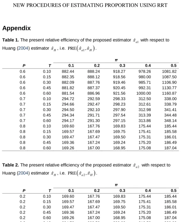
This illustration is provided to give a tangible idea about the magnitude of the relative efficiency of the suggested procedures with respect to the Huang (2004) and direct estimator procedures. The percent relative efficiency (PRE) of the proposed estimators



 

ˆ_a1,ˆ_a2



in relation to the Huang (2004) estimator



ˆ_H are given by







 















 





2 1 2 2 1 1 1 1 ˆ ˆ PRE , 100 2 1 1 1 1 a H P P P P T P P P T           _{    }       _      _ (33) and







 

 











 

 







2 2 2 1 2 1 1 1 1 ˆ ˆ PRE , 100 2 1 1 1 1 a H P P P P T P P P T             _      _    _      _ , (34)

respectively. The PRE of the proposed estimators

 

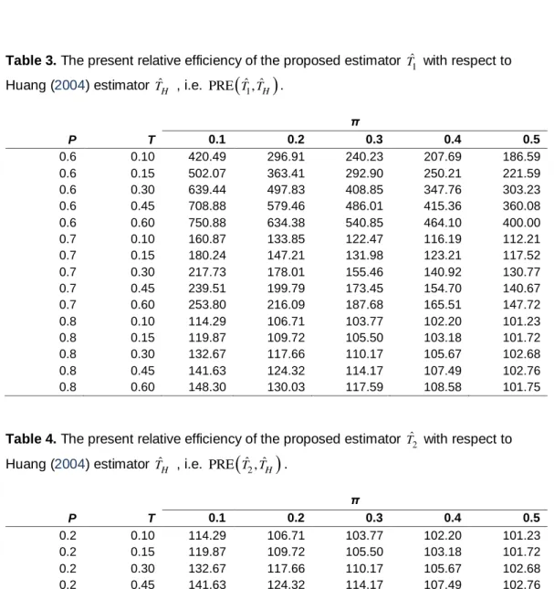
T Tˆ ˆ₁, ₂ with respect to the Huang (2004) estimator Tˆ_H are given by



1



_



_{ }

2



_



2

_



_{ }

 



_

1 2 1 1 1 ˆ ˆ PRE , 100 2 1 1 1 1 H P T P P P T T T T P T P P T T       _{    }       _      _ (35) and



2





_

 

_{ }

2



_



2

_



_



_



1 1 2 1 1 1 ˆ ˆ PRE , 100 2 1 1 1 1 H P T P TP P T T T P T P PT T         _      _    _      _ , (36)

respectively. The expression for PRE of the proposed estimators



 

ˆa1, ˆa2



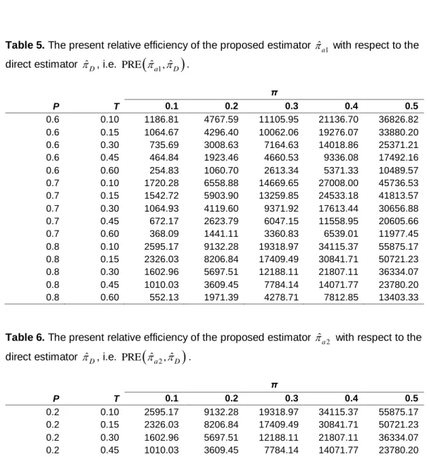
in

relation to the direct estimator ˆD are given by







_



_{ }



_







_

2 2 1 1 1 ˆ ˆ PRE , 100 1 1 1 a D P T T n T P P T           _{  }           (37) and







_





_{ }



_



_





_



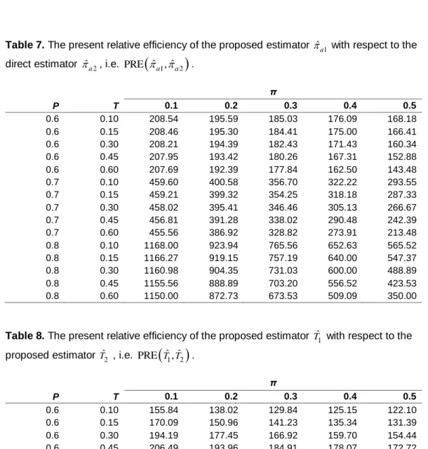
2 2 2 1 1 1 ˆ ˆ PRE , 100 1 1 1 a D P T T n T P P T             _    _        , (38)

respectively. For comparing the two proposed procedures, we give the PRE of



ˆ ,a1 Tˆ1



with respect to



ˆ ,a2 Tˆ2



as



1 2



_



_{ }

 

_





_{ }



_

1 1 1 ˆ ˆ PRE , 100 1 1 1 1 a a P P P T P P T P





 

 





 

                     (39) and

 



_

 

_{ }

_{ }



2



_{ }



_

1 2 ₂ 1 1 1 ˆ ˆ PRE , 100 1 1 1 1 P P T T PT T T T P T T P T T P



 



 

                     , (40)

respectively. We have further obtained the expressions for PRE of the proposed estimators



ˆ ,_a2 Tˆ₂



with respect to



ˆ ,_a1 Tˆ₁



, given by



2 1

 

_



_{ }



 

_

_



_



1 1 1 1 ˆ ˆ PRE , 100 1 1 1 a a P P P T P P P T





 

 





 

 _      _            (41) and

 



_



_{ }



 

_

 

_

2

_



2 1 ₂ 1 1 1 1 ˆ ˆ PRE , 100 1 1 1 P P T T P T T T T P P T T PT T



 



 

   _      _            , (42) Respectively.

Using the formulae (33)-(42), we have computed

(i) The PRE



 

ˆa1, ˆH



and PRE



T Tˆ ˆ1, H



for the values of P = 0.6, 0.7, 0.8; T = 0.10, 0.15, 0.30, 0.45, 0.60; and π = 0.1 (0.1) 0.9. The results are displayed in Tables 1 and 3.

(ii) The PRE



 

ˆa2, ˆH



and PRE



T Tˆ ˆ2, H



for the values of P = 0.20, 0.30, 0.40; T = 0.10, 0.15, 0.30, 0.45, 0.60; and π = 0.1 (0.1) 0.9. The results are shown in Tables 2 and 4.

(iii) The PRE



 

ˆa1, ˆD



for the values of P = 0.60, 0.70, 0.80; T = 0.10, 0.15, 0.30, 0.45, 0.60; π = 0.1 (0.1) 0.9; and n = 1000. The findings are displayed in Table 5.

(iv) The PRE



ˆa2,TˆD



for the values of P = 0.2, 0.30, 0.40; T = 0.10, 0.15, 0.30, 0.45, 0.60; π = 0.1 (0.1) 0.9; and n = 1000. The findings are displayed in Table 6.

(v) The PRE



 

ˆa1, ˆa2



and PRE



T Tˆ ˆ1, 2



for the values of P = 0.6, 0.7,

0.8; T = 0.10, 0.15, 0.30, 0.45, 0.60; and π = 0.1 (0.1) 0.9. The findings are displayed in Tables 7 and 8.

(vi) The PRE



 

ˆ_a2, ˆ_a1



and PRE



T Tˆ ˆ₂, ₁



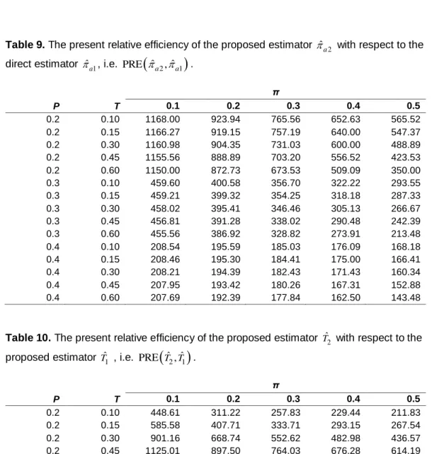
for the values of P = 0.20, 0.30, 0.40; T = 0.10, 0.15, 0.30, 0.45, 0.60; and π = 0.1 (0.1) 0.9. The results are displayed in Tables 9 and 10.

Tables 1 and 3 show that the values of PRE



 

ˆ_a1, ˆ_H



and PRE



T Tˆ ˆ₁, H



are larger than 100, showing that



ˆ_H is more efficient than



ˆ_a1 and that Tˆ₁ is also superior

to Tˆ_H . It is observed that, for fixed values of (P, T), the



ˆ 1 ˆ





ˆ ˆ1



PRE

 

a , H PRE T T, H  decreases (increases) as π increases (decreases) slowly (rapidly). For fixed values of (T, π), both PRE



 

ˆa1, ˆH



and PRE



T Tˆ ˆ1, H



decrease in a speedy manner as P increases. Thus a larger gain in efficiency by using



ˆ_a1

 

Tˆ₁ over



ˆ_H

 

Tˆ_H is expected when P is close to 0.5.

Tables 2 and 4 exhibit that

 For fixed values of (P, T), the PRE



 

ˆ_a2, ˆ_H



_PRE



T Tˆ ˆ₂, _H



_

increases (decreases) as π increases (decreases)

 PRE



 

ˆa2, ˆH



PRE



T Tˆ ˆ2, H



 decreases (increases) slowly (rapidly) as T increases (decreases)

 Both PRE



 

ˆa2, ˆH



and PRE



T Tˆ ˆ2, H



increase in a speedy way as P increases

Hence higher gain in efficiency by using ˆ_a2

 

Tˆ2 is observed when (P, π) are

closer to 0.5. It is further observed from Tables 2 and 4 that the values of



ˆ 2 ˆ



PRE

 

_a , _H and PRE



T Tˆ ˆ₂, _H



are greater than 100, from which it follows that the envisaged estimators



ˆ ,a2 Tˆ2



are more efficient than Huang’s (2004)

estimators



ˆ ,_H Tˆ_H



.

It is observed from Table 5 that

 For fixed (P, π), the PRE



 

ˆ_a1, ˆ_D



decreases as T increases

 For fixed (T, π), the PRE



 

ˆa1, ˆD



increases as P increases

There is substantial gain in efficiency through use of the proposed estimator ˆ_a1 over direct estimator ˆ_D for all values of (P, π, T) considered here.

It is observed from Table 6 that

 For fixed (P, T), the PRE



 

ˆ_a2, ˆ_D



increases as π increases

 For fixed (P, π), the PRE



 

ˆa2, ˆD



decreases as T increases

 For fixed (T, π), the PRE



 

ˆa2, ˆD



increases as P increases

There is substantial gain in efficiency through use of the proposed estimator ˆ_a2 over direct estimator ˆ_D for all values of (P, π, T) considered here.

Tables 5 and 6 clearly demonstrate the superiority of the proposed estimators

1

ˆ_a



and ˆa2 over the usual direct estimator ˆD as the values of PRE



 

ˆa1, ˆD



and



ˆ 2 ˆ



PRE

 

_a , _D are larger than 100 for all values of (P, π, T) considered.

Tables 7 and 8 demonstrate that the values of PRE



 

ˆa1, ˆa2



and



ˆ ˆ1 2



PRE T T, are greater than 100 for 0.10 ≤T≤ 0.60, 0.10 ≤T≤ 0.50, and P > 1/2. Both PRE



 

ˆa1, ˆa2



and PRE



T Tˆ ˆ1, 2



increase in a speedy way as P

increases. Hence higher gain in efficiency by using PRE



 

ˆa1, ˆa2



and



ˆ ˆ1 2



PRE T T, is observed when (P, π) are closer to 0.5.

It is observed from Tables 9 and 10 that the values of PRE



 

ˆa2, ˆa1



and



ˆ ˆ2 1



PRE T T, are greater than 100 for 0.10 ≤T≤ 0.60, 0.10 ≤T≤ 0.50, and P < 1/2. Thus the proposed procedures



ˆ ,a2 Tˆ2



are more efficient than the

estimators



ˆ ,_a1 Tˆ₁



. Higher gains in efficiencies are observed for lower values of P (i.e. for the values of P close to zero).

Finally we conclude that the proposed procedures are superior to the Huang (2004) procedure and hence the Chang and Huang (2001) procedure, and to the usual direct procedure.

Conclusion

Randomized response procedures are attractive mechanisms for counteracting fears in response and providing with valid statistical inferences concerning a population. The proposed randomized response procedure allows us to estimate the population proportion π unbiasedly and to get an admissible estimator for T, which is an unattainable feature for most of the competing methods. It has been shown theoretically and empirically that the proposed procedures are better than the Warner (1965), Chang and Huang (2001), and Huang (2004) procedures. The unbiased estimators of the MSE are provided for the direct response survey based on the proposed RR techniques. The suggested procedure is therefore recommended for application in survey sampling practice.

References

Chang, H. J. & Huang K. C. (2001). Estimation of proportion and sensitivity of a qualitative character. Metrika, 53(3), 269-280. doi: 10.1007/s001840100109

Chang, H. J., Wang, C. L., & Huang, K. C. (2004a). On estimating the proportion of a qualitative sensitive character using randomized response

sampling. Quality and Quantity, 38(5), 675-680. doi: 10.1007/s11135-005-8105-4

Chang, H. J., Wang, C. L., & Huang, K. C. (2004b). Using randomized response to estimate the proportion and truthful reporting probability in a

dichotomous finite population. Journal of Applied Statistics, 31(5), 565-573. doi:

10.1080/02664760410001681819

Chua, T. C. & Tsui, A. K. (2000). Procuring honest responses indirectly. Journal of Statistics Planning and Inference, 90(1), 107-116. doi: 10.1016/S0378-3758(00)00109-9

Fox, J. A. & Tracy, P. E. (1986). Randomized response: A method of sensitive surveys. Newbury Park, CA: SEGE Publications.

Huang, K. C. (2004). Survey technique for estimating the proportion and sensitivity in a dichotomous finite population. Statistica Neerlandica, 58(1),

75-82. doi: 10.1046/j.0039-0402.2003.00113.x

Mahmood, M., Singh, S. & Horn, S. (1998). On the confidentiality

guaranteed under randomized response sampling: A comparison with several new techniques. Biomedical Journal, 40(2), 237-242. doi:

Mangat, N. S. (1994). An improved randomized response strategy. Journal of the Royal Statistical Society. Series B, 56(1), 93-95.

Mangat, N. S. & Singh, R. (1990). An alternative randomized procedure. Biometrika, 77(2), 439-442. doi: 10.1093/biomet/77.2.439

Sing, S., Singh, R., and Mangat, N. S. (2000). Some alternative strategies to

Moor’s model in randomized response model. Journal of Statistical Planning and

Inference, 83(1), 243-255.

Singh, H. P. & Tarray, T. A. (2012). A stratified unknown repeated trials in

randomized response sampling. Commmunications for Statistical Applications

and Methods, 19(6), 751-759. doi: 10.5351/CKSS.2012.19.6.751

Singh, H. P. & Tarray, T. A. (2013a). A modified survey technique for estimating the proportion and sensitivity in a dichotomous finite population. International Journal of Advanced Scientific and Technical Research, 3(6), 459-472.

Singh, H. P. & Tarray, T. A. (2013b). An alternative to Kim and Warde’s

mixed randomized response model. Statistics and Operations Research

Transactions, 37(2), 189-210.

Singh, H. P. & Tarray, T. A. (2013c). An alternative to Kim and Warde’s mixed randomized response technique. Statistica, 73(3), 379-402.

Singh, H. P. & Tarray, T. A. (2014a). An alternative to stratified Kim and

Warde’s randomized response model using optimal (Neyman) allocation. Model

Assisted Statistics and Applications, 9(1), 37-62.

Singh, H. P. & Tarray, T. A. (2014b). An improved mixed randomized response model. Model Assisted Statistics and Applications, 9(1), 73-87.

Singh, H. P. & Tarray, T. A. (2014c). A dexterous randomized response model for estimating a rare sensitive attribute using Poisson distribution. Statistics & Probability Letters, 90, 42-45. doi: 10.1016/j.spl.2014.03.019

Singh, H. P. & Tarray, T. A. (2014d). A modified mixed randomized response model. Statistics in Transition new series, 15(1), 67-82.

Singh, H. P. & Tarray, T. A. (2014e). An improvement over Kim and Elam stratified unrelated question randomized response model using Neyman

allocation. Sankhya B, 77(1). doi: 10.1007/s13571-014-0088-5

Singh, R. & Mangat, N. S. (1996). Elements of survey sampling (Vol. 15). Dordrecht, Netherlands: Kluwer Academic Publishers.