Assessment and Improvement of a Sequential Regression Multivariate Imputation Algorithm.

Regression Multivariate Imputation Algorithm

by Jian Zhu

A dissertation submitted in partial fulfillment of the requirements for the degree of

Doctor of Philosophy (Biostatistics)

in The University of Michigan 2016

Doctoral Committee:

Professor Trivellore E. Raghunathan, Chair Professor Michael R. Elliott

Professor Susan A. Murphy Associate Professor Lu Wang

I am extremely thankful to my advisor, Professor Trivellore Raghunathan (Raghu). Without his long-term support, I would have never been able to complete my dis-sertation research. His philosophy of life and statistics are truly inspirational to me, and I greatly appreciate the advice he has given me throughout the years. I will always look upon on him as my role model in my future work.

I am very lucky to have a great and impressive committee. Each member, Pro-fessor Trivellore Raghunathan, ProPro-fessor Michael Elliott, ProPro-fessor Lu Wang and Professor Susan Murphy, has given me much great advice. I am very grateful for their feedback on shaping my research goals and revising my thesis.

I am very thankful to Dr. Hiroko Dodge, who gave me the opportunity to work with her at Michigan Alzheimer’s Disease Center. I have gained a lot of first-hand experience in medical related research through extensive collaboration work with her and her teams.

I would also like to thank the Department of Biostatistics at University of Michi-gan for its long-term support.

Last but not least, I would like to thank my entire family.

DEDICATION . . . ii

ACKNOWLEDGEMENTS . . . iii

LIST OF FIGURES . . . vi

LIST OF TABLES . . . vii

CHAPTER I. Introduction . . . 1

1.1 Missing Data Background . . . 1

1.2 Sequential Regression Multivariate Imputation (SRMI) . . . 4

1.2.1 Issues . . . 5

1.3 Thesis Layout . . . 6

II. Convergence Properties of SRMI for Single Variable Missing Patterns . . 8

2.1 Introduction . . . 9

2.2 Classification of Regression Model Sequences . . . 14

2.3 Bivariate Missing Data . . . 17

2.4 Simulation Studies for a Bivariate Missing Data . . . 26

2.5 Non-ignorable Missing Data Mechanism . . . 32

2.6 Multivariate Missing Data . . . 33

2.6.1 Single Variable Missingness . . . 34

2.7 Discussion . . . 36

2.8 Supplemental Materials . . . 45

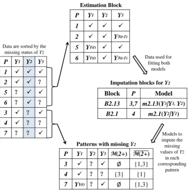
III. Block Sequential Regression Multivariate Imputation Algorithm (BSRMI) 49 3.1 Introduction . . . 50

3.2 BSRMI Algorithm . . . 55

3.3 Convergence Properties . . . 62

3.3.1 Notation . . . 62

3.3.2 Asymptotic Approximation of BSRMI . . . 64

3.4 Simulation Studies . . . 68

3.4.1 Trivariate Poisson Case . . . 68

3.4.2 Complex Case . . . 71

3.5 Discussion . . . 74

IV. Sequential Quasi-Likelihood Regression Multivariate Imputation (SQL-RMI) . . . 86

4.1.2 Motivating Example: SRMI for Trivariate Poisson . . . 88 4.2 Methods . . . 91 4.2.1 A Quasi-Predictive Distribution . . . 92 4.3 Simulation Studies . . . 94 4.4 Discussion . . . 100 V. Discussion. . . 103

5.1 Conclusions and Discussions . . . 103

BIBLIOGRAPHY. . . 106

Figure

2.1 Kullback-Leibler divergence curves between fitted regression models and true con-ditional densities of four sets of models for Example 2.4. . . 29 2.2 Maximum of absolute difference between empirical distributions based on multiply

imputed data and before deletion data, Fb

n,T

M I(x, y)−Fb_BDn (x, y)

_∞, from four im-putation algorithms plotted as a function of sample sizen=50, 100, 200, 500, 1000 and 10000 and the number of iterations T = 100,500,1000 for Example 2.4. . . 31 2.3 Maximum of absolute difference between empirical distributions based on multiply

imputed data and before deletion data, Fb

n,T

M I(x, y)−Fb_BDn (x, y)

_∞, from four im-putation algorithms plotted as a function of sample sizen=50, 100, 200, 500, 1000 and 10000 and the number of iterationsT = 100,500,1000 when the data are not missing at random in Example 2.4. . . 33 3.1 Imputing missing values forY1 at iterationt. . . 60

3.2 Imputing missing values forY2 at iterationt. . . 61

3.3 Kullback-Leibler divergence between empirical distributions, based on multiply im-puted data Fb

n,T

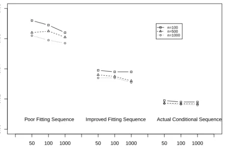
M I(x, y) and before deletion data Fb_BDn (x, y) and averaged over 500 replicates of data sets, from three imputation algorithms plotted as a function of sample size n=500, 1000, and 5000 and the number of iterationsT = 50,100,1000 when the data are missing at random. The three imputation algorithms impute the missing values in the order ofY1,Y2 andY3: the poor sequence assumes linear

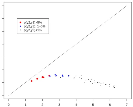
predictors only, the improved sequence assumes appropriate non-linear terms of the predictors, and the validly specified sequence assumes true conditional models from the data population. . . 72 4.1 The relation between mean and variance ofy1|y2, y3 . . . 90

4.2 Kullback-Leibler divergence between empirical distributions, based on multiply im-puted data Fb

n,T

M I(x, y) and before deletion data Fb_BDn (x, y) and averaged over 500 replicates of data sets, from three imputation algorithms plotted as a function of sample size n=500, 1000, and 5000 and the number of iterationsT = 50,100,1000 when the data are missing at random. The three imputation algorithms impute the missing values in the order ofY1,Y2 andY3: the poor sequence assumes linear

predictors only, the improved sequence assumes appropriate non-linear terms of the predictors, and the validly specified sequence assumes true conditional models from the data population. . . 101

Table

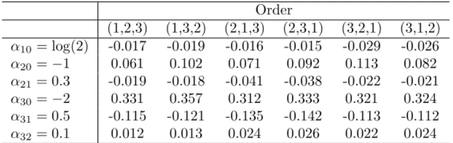
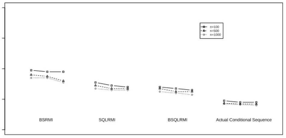
3.1 Bias in the parameter estimates based on BSRMI using the improved algorithm under different orders, Replicates=500, Imputations=20, Sample size=10,000 . . . 71 3.2 Performance of four multiple imputation algorithms on the example in Chen et al.

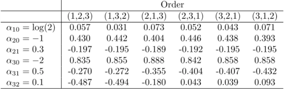
(2011), R=500, M=5 . . . 73 3.3 Bias in the parameter estimates based on BSRMI using the poor fitting models

under different orders, Replicates=500, Imputations=20, Sample size=10,000 . . . 85 3.4 Bias in the parameter estimates based on BSRMI using the actual conditional

models under different orders, Replicates=500, Imputations=20, Sample size=10,000 85 4.1 Biases, RMSE and 95% confidence interval coverage rates of parameter estimates

using various approaches, R=500, M=5 . . . 99

Introduction

1.1 Missing Data Background

In many statistical studies, especially in large complex studies with many types of variables, data can be missing due to various reasons such as attrition, refusal, partial response (Little and Rubin, 2002), and study designs such as matrix sampling (Raghunathan and Grizzle, 1995) and data merging (Wang, Song and Wang, 2015). The missing values often create statistical challenges for analysts in obtaining valid inferences.

One challenge is raised by different missingness patterns. When data are presented in a wide format (rows correspond to subjects and columns correspond to variables), the data matrix displays three missingness patterns: 1. univariate pattern, 2. mono-tone pattern and 3. arbitrary pattern (Schafer and Graham, 2002). In a univariate pattern, missing values occur only on one variable and all other variables are fully observed; in a monotone pattern with ordered variables, once a variable is missing, then all succeeding variables are missing; the arbitrary pattern is the most general pattern in which different sets of variables can be missing for different subjects. This thesis focuses on the arbitrary pattern in multivariate datasets. In addition, we consider a single variable missing pattern, a special case of the arbitrary pattern in

which data are missing on up to one variable in any row and the missing variable may be different across subjects. Unlike the first two patterns, which can be han-dled by simple methods, the arbitrary pattern and its special case may require more sophisticated approaches.

Another challenge is raised by different mechanisms that generate the missing values. Take a naive analysis approach for example, which restricts the analysis to subjects providing complete data on variables relevant for the analysis. This approach is the default method in many statistical software packages, and it is valid if the complete cases or available cases are representative of all cases. However, this strong assumption may not be true in general, and, even if true, this approach may lead to loss of efficiency. It is more likely that the inferences from the complete-case analysis will not be valid; for example, the parameter estimates may be biased.

Rubin (1976), a groundbreaking paper, proposed a missing data analysis frame-work with the definition of three types of missingness mechanisms: missing com-pletely at random (MCAR), missing at random (MAR) and not missing at ran-dom (NMAR). Furthermore, when data are MAR and the population or substantive model parameters are distinct from the parameters in the missingness mechanism, the likelihood-based inferences do not require the exact form of missingness mecha-nism. Within this framework, researchers have developed many methods to properly analyze incomplete data.

The likelihood-based methods generally adopt either frequentist maximum likeli-hood (ML) methods or fully Bayesian approaches. The Expectation-Maximization (EM) algorithm (Dempster, Laird and Rubin, 1977), and Monte Carlo simulation techniques have made implementation of these methods computationally possible for a selected set of models. The frequentist-based ML methods usually rely on large

sample size whereas the fully Bayesian methods can handle small sample sizes. The parameters of interest can be drawn from the joint posterior distribution along with the missing values by rejection sampling methods or Monte Carlo Markov Chain (MCMC) algorithms such as Gibbs sampler (Geman and Geman, 1984).

Inverse probability weighting (Little and Rubin, 2002) is another way to adjust the complete case analysis, and is especially useful for unit non-response in survey settings. An alternative is the propensity prediction method (Little and An, 2004), which uses the propensity score as a covariate instead of weights.

Both maximum likelihood and Bayesian-based methods are computationally in-tensive and require development of specialized codes. On the other hand, inverse probability methods can handle special patterns of missing data (such as univariate pattern or monotone pattern). Rubin (1977, 1987) proposed the multiple impu-tation approach, which capitalizes on the complete data software programs. The multiple imputation approach uses the observed data to estimate the distribution of the missing data, and imputes the missing values from the predictive distribution. To properly estimate the uncertainty due to filling in the missing values, multiple com-pleted data sets are created by the same imputation algorithm, and analysis results from each completed data set are combined to obtain the final inference following Rubin’s (1977) formula.

An advantage of this approach, especially when data are missing arbitrarily in a complex study, is that once the missing data are imputed, one can analyze the completed datasets as if there were no missing values by simply using existing soft-ware packages. If the same data are analyzed by various researchers, a well-imputed data source can ensure that analysis results by different researchers are consistent. This approach also can be viewed as a small simulation approximation for the fully

Bayesian analysis when the model used for the imputation is also the model for the analysis.

Numerous approaches have been developed for creating multiple imputations. Some common imputation methods include nonparametric methods such as Hot Deck imputation (Andridge and Little, 2010), and model-based methods based on a joint distribution of all variables with missing values conditional on all the variables that have no missing values. However, when a study has a complex data structure with many types of variables, skip patterns, structural dependencies etc., both Hot-deck and joint model approaches are difficult, if not impossible, to implement.

1.2 Sequential Regression Multivariate Imputation (SRMI)

When joint modeling becomes difficult in practice, an alternative is to use a se-quential regression multivariate imputation (SRMI) algorithm. This approach as-sumes a set of univariate regression models for each missing variable and has gained popularity due to its flexibility and ease of implementation. First proposed in Ken-nickell (1991), this approach is also commonly known as multiple imputation by chained equations (MICE) or multiple imputation by fully conditional specification (FCS).

The algorithm can be described as follows. Let the data set onnsubjects consist of qvariables with no missing values arranged in ann×qmatrix,U. LetY1, Y2, . . . , Ypbe

p variables with some missing values. Sequential regression multivariate imputation is an iterative approach for imputing the missing values inYj through random draws

based on fitting a regression modelP r(Yj|U, Y[−j]) whereY[−j]is all the variables with

missing values except Yj (Van Buuren and Oudshoorn, 1999, Raghunathan et al.,

distribution, P r(Yj|U, Y (t) 1 , Y (t) 2 , . . . , Y (t) j−1, Y (t−1) j+1 , . . . , Y (t−1)

p ) where Y_l(s) is the filled

in Yl at iteration s (observed or imputed). Each predictive distribution corresponds

to an appropriate regression model.

At each iteration, imputation involves two steps: (1) the regression model is fit to the observed values of the variable being imputed and all other variables (observed or imputed), and the parameters are drawn from the approximate posterior distribution; and (2) the draws from the regression model given the drawn parameters and all other variables are used as imputations for the missing values. The software IVEWARE (Raghunathan et al., 2001) implements this approach using a fully Bayesian approach (that is, Steps 1 and 2). Several other additional features such as placing bounds on the imputed values, restricting the sample to accommodate skip patterns, model tuning, and diagnostics are built into the software. A similar approach has been implemented in PROC MI in SAS (2008), MICE (Van Buuren and Oudshoorn, 1999) and MI (Su et al., 2011) in R, STATA (Royston, 2005) and SPSS (SPSS, 2009).

The sequential regression approach has two major practical advantages over other model-based imputation methods. Firstly, it enables handling of complex data struc-tures by focusing on a set of regression models with a univariate outcome. The flexi-ble selection of regression models also enaflexi-bles better prediction of the missing values based on other variables, and the regression models are more intuitive to analysts than a joint model. Secondly, individual regression models can easily account for study designs such as skip patterns, logical constraints, bounds for imputed values and consistency requirements.

1.2.1 Issues

A theoretical weakness of this approach is that the specifications of fully condi-tional distributions for a set of variables do not guarantee the existence of a joint

distribution. Theoretical assessment of SRMI is limited in the literature. In Liu et al. (2014), the convergence properties were studied when the joint distribution exists; however, this may not be the case for general SRMI by common GLMs. Empirical studies have shown that a few iterations are sufficient to utilize the predictive power of the observed covariates in creating imputations (Van Burren, 2007), but such examples are often limited to linear regression models. Similar simulation studies (Collins, Schafer and Kam, 2001) have proposed guidance for SRMI such as rec-ommending the use of the most inclusive policy; therefore, careful examination for general model specification is needed.

When the missingness is general and models other than linear regression models are used, SRMI may not work well in some cases. Li, Yu and Rubin (2012) have demonstrated the need for caution through the use of some theoretical examples. This thesis studies one motivating trivariate count variable example extensively. In particular, a simulation study shows that with poorly fit model sequences, one SRMI algorithm for this example may diverge. Therefore, the regular SRMI needs to be modified to avoid such behavior.

1.3 Thesis Layout

In order to address the issues above, this thesis work investigates the convergence properties of SRMI in various cases, and proposes modifications for improvement. It consists of the following chapters.

Chapter 2 assesses the convergence properties of SRMI for the simple case where each subject may be missing a value on at most one variable. We define several classes of generalized linear regression model sequences according to their model compatibility and validity properties. We also establish two sufficient conditions that

allow the algorithm to perform well. For all types of compatible and incompatible model sequences, we conduct simulation studies to evaluate their convergence and performance. We then use the results to develop criteria for the choice of imputation models. This chapter was published as Zhu and Raghunathan (2015).

Chapter 3 proposes a modified block sequential regression multivariate imputa-tion (BSRMI) approach to divide the data into blocks when imputing each variable based on missing data patterns and tune the regression models through compatibil-ity restrictions. This is extremely helpful to avoid divergence when it is difficult to get well-fitting models across all records with missing values for a general pattern of missing data. We establish two sufficient conditions for the convergence of the algorithm, and study the repeated sampling properties of inferences using several simulated data sets.

Chapter 4 extends the imputation model selection to quasi-likelihood regression models in both SRMI and BSRMI, when it is difficult to identify a well-fitting gener-alized linear model sequence. We examine the performance of the modified approach through simulation studies. We demonstrate that the new approach can be used to improve repeated sampling properties due to their improved model prediction.

Finally, Chapter 5 summarizes the findings and discusses limitations and future work.

Convergence Properties of SRMI for Single Variable Missing

Patterns

Abstract

A sequential regression or chained equations imputation approach uses a Gibbs sampling type iterative algorithm which imputes the missing values using a sequence of conditional regression models. It is a flexible approach for handling different types of variables and complex data structures. Many simulation studies have shown that the multiple imputation inferences based on this procedure have desirable repeated sampling properties. However, a theoretical weakness of this approach is that the specification of a set of conditional regression models may not be compatible with a joint distribution of the variables being imputed. Hence, the convergence properties of the iterative algorithm are not well understood. This chapter develops conditions for convergence and assesses the properties of inferences from both compatible and incompatible sequence of regression models. The results are established for the miss-ing data pattern where each subject may be missmiss-ing a value on at most one variable. The sequence of regression models are assumed to be empirically good fit for the data chosen by the imputer based on appropriate model diagnostics. The results are used to develop criteria for the choice of regression models.

Key Words: Bayesian analysis; Chained equations, Compatible conditionals; Conditional specifications; Exponential family; Gibbs sampling; Missing data; Mul-tiple imputation

2.1 Introduction

Consider a data set with p variables, Y1, . . . , Yp, with some missing values. The

sequential regression (or chained equations, flexible conditional specifications) impu-tation approach uses a Gibbs sampling style iterative algorithm where, at iteration t = 1, . . . , T, the imputations for missing values in variable Yi are drawn from the

posterior predictive distribution,

p(Yi |Y (t) 1 , . . . , Y (t) i−1, Y (t−1) i+1 , . . . , Y (t−1) p ),

whereY_j(t)equals the observed value, if available, or an imputed value at iterationt, if missing. DenotingY_[(₋t)_i]={Y₁(t), . . . , Y_i(₋t)₁, Y_i(₊₁t−1), . . . , Yp(t−1)}, the posterior predictive

distribution corresponds to a parametric regression model,p(Yi |θi, Y

(t)

[−i]) and a prior

distribution π(θi). Denoting Yi,obs and Yi,mis as the observed and missing values of

Yi, the following two step procedure is used to draw the missing values:

Step 1: Draw a value ofθi, say,θi∗, from its posterior densityπ(θi |Yi,obs, Y

(t) [−i]).

Step 2: Draw the set of missing valuesYi,misfrom the modelp(Yi |θi∗, Yi,obs, Y

(t) [−i]).

For large samples, the first step may be skipped and the maximum likelihood or any other consistent estimate of θi may be used in the second step. This approach

is not Bayesianly proper and may result in understating the variability among the imputed values but may be negligible for large samples. Since our interest is in establishing the asymptotic convergence properties, we skip the draw in Step 1 and

use a consistent estimate of θi obtained from the data {Yi,obs, Y

(t)

[−i]} (typically the

maximum likelihood estimate θb

(t)

i ) in Step 2.

The sequential regression approach was first used by Kennickel (1991) for imputing the missing values in continuous variables in the Survey of Consumer Finances using a sequence of linear regression models. Brand (1999), Van Buuren and Oudshoorn (1999) and Raghunathan et al. (2001) generalized this approach by considering linear regression for continuous, logistic for binary, multinomial logit for more than two categories, Poisson for count and a two-stage model (logistic and then conditional normal) for semi-continuous variables which are generally continuous but have a spike at 0 (For example, real estate income, it is zero for a sizable fraction of the population and a continuous value for the rest).

The sequential regression approach has two major practical advantages over other model-based imputation methods. It enables handling of complex data structures by focusing on a set of regression models with a univariate outcome. The flexible selection of regression models enables better prediction of the missing values based on other variables, and the regression models are more intuitive to analysts than a joint model. Also, individual regression models can easily account for study designs such as skip patterns, logical constraints, bounds for imputed values and consistency requirements. The software IVEWARE (Raghunathan et al., 2001) implements this approach using a fully Bayesian approach (that is, Steps 1 and 2). Several other additional features such as placing bounds on the imputed values, restricting the sample to accommodate skip patterns, model tuning and diagnostics are built into the software. A similar approach has been implemented in PROC MI in SAS (2008), MICE in the R package(Van Buuren and Oudshoorn, 1999) and in STATA (Royston, 2005). The recent issue of the Journal of Statistical Software (2012) has published

several articles on this approach.

A theoretical weakness of this approach is that the specifications of conditional dis-tributions for a set of variables do not guarantee the existence of a joint distribution, and hence, it is not clear whether the iterative algorithm will achieve any stability. The convergence results established for the standard Gibbs sampling algorithms or its variations may not be applicable. This problem was also discussed in the context of spatial analysis (Besag, 1974), and the necessary and sufficient conditions for the existence of a joint model were given by Arnold and Press (1989) for bivariate con-ditional densities. Gelman and Speed (1993) also discussed the existence of a unique joint distribution given a set of conditional and marginal distributions. Arnold et al. (2001) gave a thorough introduction to the problem in general, and Gelman and Raghunathan (2001) joined the discussion regarding the effect of incompatible conditionally specified models in missing data analysis.

In the sequential regression imputation context, Van Buuren et al. (2006) showed through simulations that incompatibility caused minimal effects in some cases. Drech-sler and RasDrech-sler (2008) showed that choosing poorly fitting incompatible models may lead to biased estimation. From a theoretical perspective, Li et al. (2012) used incom-patible regression models with fixed parameters to illustrate that model incompati-bility may or may not necessarily imply algorithmic incompatiincompati-bility (convergence). However, they fix the parameters across all the iterations but in the sequential regres-sion approach parameters change with iterations. That is, the sequential regresregres-sion approach is a Markov type process. Liu and Gelman (2013) established technical conditions for the convergence of the sequential regression approach if the station-ary joint distribution exists. In practice, however, the models may be chosen where the stationary joint distribution may not exist. Hence, we need to investigate the

convergence properties under more general conditions.

The incompatibility may not lead to divergence can be illustrated using the follow-ing bivariate example. Suppose that the data set with two variables (X, Y) can be di-vided into three groups: thenXY individuals with both (X, Y) observed, thenX

indi-viduals with missingY and thenY individuals with missingX. Assume that the

miss-ing data mechanism is ignorable as defined in Rubin (1976). After an empirical in-vestigation, suppose that an imputer decides to usem1(y|x, θ1)∼exponential(θ1x)

and m2(x | y, θ2) ∼ exponential(θ2y) as conditional regression models. There is

no joint distribution with these two conditional distributions. At iteration t, the imputation of missing Y is drawn from exponential(θb

(t) 1 x) where b θ₁(t) = (nXY +nY)/( X i∈RXY xiyi+ X i∈RY x(_it−1)yi),

and the imputed values for the missing X is drawn from exponential(θb

(t) 2 y) where b θ(₂t) = (nXY +nX)/( X i∈RXY xiyi+ X i∈RX xiy (t) i ).

Let ρXY, ρX and ρY be the limiting values of nXY/n, nX/n and nY/n, respectively,

as n→ ∞. The above two equations, in the limit, are

θ₁(t) = (ρXY +ρY)/(ρY/θ

(t−1)

2 +ρXYEo),

and

θ(₂t) = (ρXY +ρX)/(ρX/θ(1t)+ρXYEo).

where Eo is the expected value of the product XY for the complete cases. It is easy

to show that the limiting case of the iterative algorithm given above converges to θ₁∗ = θ∗₂ = 1/Eo. Thus asymptotically, as the sample size, n, the number of

joint density function (X, Y) averaged over infinite number of imputations,fM I(x, y),

tends to ρXYfo(x, y) + (ρYyf1(y) +ρXxf2(x)) exp(−xy/Eo)/Eo wherefo(x, y) is the

joint density of (X, Y) for complete cases,f1(y) is the marginal density ofY for

sub-jects with missingX andf2(x) is the marginal density ofX for subjects with missing

Y. Thus, the practical validity of the multiple imputation inferences depends on the closeness of m1(y | x, θ1) and m2(x | y, θ2) to the corresponding true conditional

distributions f1(y | x) and f2(x | y). Under the missing at random assumption,

if the model diagnostics based on the observed data indicate a good fit of the two conditional exponential distributions then the incompatibility may have a very little practical impact on the inferences. For example, if the true joint density function of (X, Y) is f(x, y) ∝ exp(−xy/Eo−x−y) where is an arbitrarily small positive

number, then an imputer is likely to choose the two conditional models given above. In this case, fM I(x, y) is nearly the same as f(x, y) depending upon the .

On the other hand, suppose that the true joint density function of (X, Y) is f(x, y)∝ exp(−αxy−βx−γy) with α > 0, β >0 and γ > 0. The two conditional distributions are exponential distributions with αx+β as the parameter forf(y|x) and αy+γ as the parameter off(x|y) (Arnold and Strauss, 1988) . Again, assume that the missing data mechanism is ignorable and that the imputations are carried out under the following sequence of regression models, m(x|y)∼exponential(φ1+

φ2y) andm(y|x)∼exponential(φ3+φ4x). These two conditional distributions are

not compatible with any joint distribution unless φ2 =φ4. Note that the functional

form of the two conditional densities match the true densities, and the two conditional densities are compatible when (φ2 = φ4 > 0, φ1 > 0 and φ3 > 0), a subspace of

the joint parameter space (φi > 0, i = 1,2,3,4) used by the imputer. We may

embedded within the joint parameter space of the conditional distributions used in the imputation process. For such situations, Theorem 2.1 given in the next section provides sufficient conditions for the sequential regression imputation approach to yield a consistent estimator of the joint density function of (x, y). In fact, many standard conditional regression models satisfy the sufficient conditions.

The rest of the chapter is organized as follows. Section 2.2 provides definition of incompatibility and model validity to classify regression models in the sequen-tial regression approach. Section 2.3, focusing on bivariate scenario, provides two sufficient conditions for the convergence of the sequential regression approach and obtain consistent estimators. Section 2.4 enhances the analytical results given in Sections 3 through a simulation study for incompatible but approximately valid or well fitting model sequences. Section 2.5 considers the convergence properties under nonignorable missing data mechanisms. Section 2.6 extends the results for multi-variate missing data with single variable missing data pattern (that is, any subject is missing at most one variable). Section 2.7 summarizes the findings, discusses ex-tensions for arbitrary pattern of missing data and the limitation of the sequential regression algorithm.

2.2 Classification of Regression Model Sequences

Before we establish the convergence and consistency properties, we define the de-gree or types of incompatibility among the conditionally specified regression model in the sequential regression algorithm. We consider two types of incompatible mod-els, one with reference to the true or actual distribution and another without any reference to the true distribution. The former is of more theoretical interest or when the posited joint distribution is too complicated and an imputer would like to find

an approximately valid sequential regression model. The latter is tuned towards selecting the kind of sequential regression models that will lead to convergence.

Definition 1 (Weakly Incompatible Model Sequence): Supposes that the

joint density function,f(y1, . . . , yp) has the conditional densitiesf(yi |y[−i], ψi),

i = 1,2, . . . , p. A regression model mi(yi | y[−i], θi) with θi ∈ Θi is defined to

be validly specified for f(yi | y[−i], ψi) if the following condition holds: for any

ψi, θi can be expressed as (g(ψi), ξi), and there exists θi0 = (g(ψi),0)∈Θi such

that mi(yi |y[−i], θi0) =f(yi |y[−i], ψi).

A sequence of regression models is defined to be weakly incompatible if each regression model in the sequence is validly specified.

For example, bothm(y|x, θ)∼N(θ10+θ11x, σ2) andm(y|x, θ)∼N(θ10+θ11x+

θ12x2, σ2) are validly specified models for the conditional density y|x∼N(2 +x,1).

The former is exactly specified, and the latter has an extra term with the parameter ξ =θ12.

Definition 2 (Possibly Compatible Models): A sequence of regression

models mi(yi | y[−i], θi), θi ∈ Θi is defined to be possibly compatible, if there

exists a target joint density function p(y1, . . . , yp | θ) with conditional density

functions, pi(yi |y[−i], θYi|Y[−i]) for i= 1,2, . . . , p such that the exact functional

form of mi is the same as pi for some subspace ΘC ⊆Θ1×Θ2 × · · · ×Θp and

(θY1|Y[−1], . . . , θYp|Y[−p]) can be functionally expressed in terms of (θ1, θ2, . . . , θp).

Two linear regression models, m1(y|x, θ1)∼N(θ1o+θ11x, σ212) and m2(x|y, θ2)∼

N(θ20+θ21y, σ212 ) are weakly compatible if θ11/σ122 −θ21/σ221= 0, θ2116=σ122 /σ212 and

θ2

21 6=σ212 /σ212, where the first equation ensures thatm1(y|x, θ1)/m2(x|y, θ2) can be

are integrable. They are also possibly compatible if the target joint distribution is a bivariate normal distribution.

A subclass of possibly compatible model sequence with separate parameters for marginal and conditional distributions is defined below. Anderson (1958) used the separable parameters to develop maximum likelihood estimates for the mean and the covariance matrix of the multivariate normal distribution with a monotone pattern of missing data.

Definition 3 (Possibly Compatible Model Sequence With Separable Marginal Parameters): A joint density function p(y1, . . . , yp | θ) is defined

to have separable marginal parameters if for any subsetYM of Y ={y1, . . . , yp},

θYC|YM is distinctive from θYM, where YC = Y −YM, θYC|YM is from the

condi-tional distributionp(YC |YM, θYC|YM) andθYM is from the marginal distribution

p(YM | θYM). Equivalently, separable marginal parameters imply that for the

parameterization (θYM, θYC|YM), the parameter space is the product of two

inde-pendent parameter spaces Θ = ΘYM ×ΘYC|YM.

A sequence of possibly compatible regression models is defined to have separable marginal parameters if the target joint density function has separable marginal parameters.

As an example, suppose that (Y1, . . . , Yp) is ap-dimensional continuous variable,

and the model sequence consists of

mi(yi |y[−i], θi)∼N(θi0 +

X

j6=i

θijyj, σi2), i= 1, . . . , p.

The target joint distribution is a multivariate normal distribution and the nec-essary compatibility condition is that for any i 6= j, θij/σi2 −θji/σj2 = 0. The

mM(yM) ∼ M V N(µM,ΣM) and for any yi ∈ YC = Y −YM, mi(yi | y[−i], θi) ∼

N(θi0 +P_j6=iθijyj, σ

2

i).

Suppose that (Y1, . . . , Yp) is ap-dimensional binary variable, and model sequence

consists of mi(yi |y[−i], θi)∼Bernoulli   1 + exp −θi0 − X j6=i θijyj − X j6=i,k6=i,k<j θijkyjyk !!−1 ,

where i= 1,2, . . . , p. The target joint distribution is a multivariate Bernoulli distri-bution and the compatibility condition is that for any different i, j and k, θij =θji

and θijk = θjik = θkij. The marginal parameters are separable as follows: for any

subset YM of Y ={y1, . . . , yp}, YM follows a multivariate Bernoulli distribution and

for any yi ∈YC =Y −YM, mi(yi |y[−i], θi)∼Bernoulli   1 + exp −θi0 − X j6=i θijyj − X j6=i,k6=i,k<j θijkyjyk !!−1 .

In summary, Definition 1 classifies all regression model sequences into valid and invalid sequences with reference to the true joint density function of the variables being imputed; Definition 2 classifies model sequences into possibly compatible and incompatible sequences regardless of the true underlying joint distribution of the variables. The possibly compatible sequence has a target joint density function within the parameter space; Definition 3 defines a subclass of possibly compatible sequences based on the property of the target joint distribution’s marginal parameter property.

2.3 Bivariate Missing Data

Before we consider the multivariate imputation problem, we consider the bivari-ate case, mostly for notational simplicity and ease of presentation. For now, we assume that the missing data mechanism is ignorable as in Rubin (1976) and all

the conditional distributions belong to the exponential family. We consider non-ignorable missing data mechanisms in Section 2.5. The convergence and consistency are asymptotic properties as the sample size, the number of imputation and the number of iterations or sequential updates all tend towards ∞.

Suppose that (X, Y) follows a joint distribution with the joint density fXY(x, y |

ψ), the marginal densities fX(x |ψX) and fY(y |ψY), and the conditional densities

fY|X(y|x, ψ1) and fX|Y(x |y, ψ2). Let R denote the response pattern where R = 0

consists of complete cases {(x0i, y0i)}, i = 1, . . . , n0; R = 1 consists of cases with

missing X but observed Y, {y1j, j = 1, . . . , n1}; and R = 2 consists of cases with

missing Y but observed X, {x2k, k = 1, . . . , n2}. The missing data to be imputed

consists of {x1j, j = 1, . . . , n1} when R = 1 and {y2k, k = 1, . . . , n2} when R = 2.

The total sample size is n = n0 +n1+n2. We also assume that the proportion of

missing data will be nontrivial in a sense that as n→ ∞, n0/n →ρand n1/n→ρ1,

where 0 < ρ < 1 and 0 < ρ1 < 1−ρ. We denote Pr(R = 1 | X, Y) = g1(y),

Pr(R = 2 | X, Y) = g2(x) and Pr(R = 0 | X, Y) = 1 − g1(y) − g2(x), where

parameters in g1 and g2 are distinct from ψ, the parameters in the complete data

model. It is easy to show that f(x | y, R = 1) = f(x | y, R 6= 1) = fX|Y(x | y, ψ2),

and f(y|x, R= 2) =f(y |x, R6= 2) =fY|X(y|x, ψ1).

The sequential regression imputation algorithm assumes a regression modelm1(y|

x, θ1) for y given x and m2(x|y, θ2) for x given y respectively. We assume that the

regression models are generalized linear models from the exponential family:

m1(y|φ1, δ1, x) = exp T1(y)Tφ1−b1(φ1) /a1(δ1) +c1(y, δ1) , m2(x|φ2, δ2, y) = exp T2(x)Tφ2−b2(φ2) /a2(δ2) +c2(x, δ2) ,

condi-tional means and predictor variables through h−₁1(PU u=0θ1uh1u(x)) = b 0 1(φ1) and h−₂1(PV v=0θ2vh2v(y)) = b 0 2(φ2).

At iterationt, the algorithm is executed in two steps:

Step 1: θ1(t)is estimated by regressing{y0i, y1j}on{x0i, x

(t−1)

1j }with modelm1,

and the missing values ofy, {y₂(t_k)}, are drawn from the conditional distribution m1(y| {x2k}, θ

(t) 1 );

Step 2: θ2(t) is estimated by regressing {x0i, x2k} on updated {y0i, y

(t)

2k} with

modelm2, and the missing values ofX,{x (t)

1j}, are drawn fromm2(x| {y1j}, θ

(t) 2 ).

To be specific, the above two steps calculate the log-likelihood functions at itera-tion t for the two models:

l1(θ1 |Xobs, Yobs, X (t−1) mis ) = X i logm1(y0i |x0i, θ1) + X j logm1(y1j |x (t−1) 1j , θ1), l2(θ2 |Xobs, Yobs, Y (t) mis) = X i logm2(x0i |y0i, θ2) + X k logm2(x2k|y (t) 2k, θ2),

and estimate the parameters (θ(₁t), θ₂(t)) by solving the score equations:

s1(θ1 |Xobs, Yobs, X

(t−1)

mis ) =∂l1(θ1 |Xobs, Yobs, X

(t−1)

mis )/∂θ1 = 0,

s2(θ2 |Xobs, Yobs, Y

(t)

mis) =∂l2(θ2 |Xobs, Yobs, Y

(t)

mis)/∂θ2 = 0.

The completed data set at iterationT consists of{(x0i, y0i),(x

(T)

1j , y1j),(x2k, y

(T) 2k )}.

Suppose θ₁(T) and θ₂(T) are the estimates of θ1 and θ2 respectively. We wish to study

the properties of these estimates as n and T tends to∞.

equations given above can be approximated by (or tend to) the following equations: ˜ s1(θ1 |θ2(t−1), ψ) = n0 Z Z _∂logm 1(y|x, θ1) ∂θ1 fXY(x, y |R= 0)dxdy +n1 Z Z _∂logm 1(y|x, θ1) ∂θ1 m2(x|y, θ2(t−1))dxfY(y|R= 1)dy. ˜ s2(θ2 |θ1(t), ψ) = n0 Z Z _∂logm 2(x|y, θ2) ∂θ2 fXY(x, y |R= 0)dxdy +n2 Z Z _∂logm 2(x|y, θ2) ∂θ2 m1(y|x, θ1(t))dyfX(x|R= 2)dx. Then both ˜s1(θ (t) 1 | θ (t−1) 2 , ψ) and ˜s2(θ (t) 1 | θ (t) 2 , ψ) converge to 0 in probability as

n → ∞, which lead to an approximate iterative algorithm ˜s1(θ (t) 1 | θ (t−1) 2 , ψ) = 0 and ˜s2(θ (t) 2 | θ (t)

1 , ψ) = 0. Therefore, the implicit recursive algorithm θ (t)

1 =

˜

s₁−1(θ₂(t−1), ψ), θ₂(t) = ˜s−₂1(θ(₁t), ψ) has the convergence property similar to that of the imputation algorithms asymptotically.

Theorem 2.1. Suppose that the imputation models are weakly incompatible as defined in the previous section and the conditional distributions satisfy the following usual regularity conditions:

1. The density functionsm1 andm2 are differentiable with respect toθ1 and θ2

respectively and the differentiation and integration are interchangeable with respect to (x,θ1) for m1 and (y, θ2) for m2 respectively

2. The mean and the variance of the score functions given above exist under both the posited (m1, m2) and the true models (fX|Y, fY|X).

Then as the sample size n, the number of imputations m and the number of iterations t tend to ∞, the regression models m1(y | x, θ

(t)

1 ) → fY|X(y | x, ψ1)

and m2(x|y, θ (t)

2 )→fX|Y(x|y, ψ2).

consider two examples to assess the convergence properties of the asymptotic iterative algorithm.

Example 2.1 (Two Linear Regression Models): Suppose the data (X, Y)

are generated from a bivariate normal distribution BVN(µ,Σ) with the condi-tional distributions y | x ∼ N(α10+α11x, τ122) and x | y ∼ N(α20+α21y, τ212).

where α11/τ122 = α21/τ212. Suppose data are missing completely at random:

π0 =pr(R = 0), π1 =pr(R = 1) and π2 =pr(R= 2). The asymptotic iterative

algorithm is calculated in Appendix 2.2. The estimated regression parameters are shown to converge to θ₁∗ = (α10, α11, τ122)T, and θ

∗

2 = (α20, α21, τ212)T. The

rate of convergence for the iterative algorithm is π1π2/{(π0+π1)(π0+π2)}.

Example 2.2 (Two Logistic Regression Models): Suppose the data (X, Y)

are generated from a bivariate Bernoulli distribution with pr(X = 0, Y = 0) = p00, pr(X = 0, Y = 1) =p01, pr(X = 1, Y = 0) =p10 and pr(X = 1, Y = 1) =

p11 = 1−p00−p01−p10, with conditional distributionsy|x∼Bernoulli{(1 +

exp(−α10−γ12x))−1} andx|y ∼Bernoulli{(1 + exp(−α20−γ21y))−1}, where

γ12 = γ21. Suppose data are missing completely at random: π0 = pr(R = 0),

π1 = pr(R = 1) and π2 = pr(R = 2). The asymptotic iterative algorithm is

calculated in Appendix 2.2. The estimated regression parameters are shown to converge to θ∗₁ = (α10, γ)T, and θ2∗ = (α20, γ)T where γ12 =γ21 =γ.

We now show the results for the possibly compatible models, where the posited conditional models may not agree with the true distributions but may be compatible with some joint distribution in a subset of the parameter space. The following theo-rem provides conditions for the convergence of the sequential regression imputation algorithm.

Theorem 2.2. Suppose a sequential regression imputation algorithm uses pos-sibly compatible models m1(y | x, θ1) and m2(x | y, θ2), with pXY(x, y | θ1, θ2)

as the joint distribution only when θ = (θ1, θ2) ∈ ΘC ⊂Θ1×Θ2. If pXY(x, y |

θ1, θ2, θ ∈ ΘC) has separable marginal parameters and (θ1∗, θ ∗

2) is the maximum

likelihood estimate of(θ1, θ2) from the joint model, then under the same

regular-ity conditions in Theorem 2.1 with respect to differentiation/integration and the existence of the mean/variance of the score functions , m1(y | x, θ(1t)) → p(y |

x, θ∗₁) and m2(x|y, θ(2t))→p(x|y, θ ∗

2) as n, t→ ∞.

The proof of this theorem is given in Part 2 of Appendix 2.1. Note that if the compatibility condition is strictly imposed when θ1 and θ2 are estimated at each

iteration, then the imputation algorithm is a simplified version of a standard Markov chain with convergence to a stationary joint distribution. However, the sequential re-gression imputation does not estimate θ1 andθ2 simultaneously within one iteration,

and the compatibility condition is ignored in the estimation process. For sequences with separable marginal parameters such as Example 2.1 and Example 2.2, since (θ1∗, θ2∗) ∈ ΘC holds inherently, according to Theorem 2.2, the compatibility

con-dition is approximately satisfied for (θ1(t), θ2(t)) after a certain number of iterations.

However, we will show that this is not always true for possibly compatible sequences without separable marginal parameters.

When a possibly compatible model sequence does not have separable marginal parameters, the marginal distributions p(x | θ1, θ2) and p(y | θ1, θ2) from the target

joint distribution also depend on regression parameters, and, hence, the log-likelihood functions from the sequential regression imputation and joint modeling imputation differ. For an heuristic explanation, consider θ1 from m1 as an example. For any

the sequential regression model, where as it is log(m1(y | x, θ1)p(x | θ1, θ2)) from

the joint model. Because the distribution of observed X involves θ1, in general, the

log-likelihood functions ofθ1from the joint model and the sequential regression differ.

Therefore, the two algorithms yield different parameter estimates and imputation results.

To clarify this aspect further, consider the following simulation examples:

Example 2.3 (Two Poisson Regression Models): Consider,m1(y|x, θ1)∼

P oisson(exp(θ10 + θ11x)) and m2(x|y, θ2) ∼ P oisson(exp(θ20 +θ21y)). The

compatibility condition requires thatθ11 =θ21<0, and the corresponding joint

distribution is m(x, y | θ1, θ2, θ11 =θ21 < 0) = c(θ10, θ20, θ11) exp(θ10y+θ20x+

θ11xy), where c(θ10, θ20, θ11) is the normalizing constant. The log-density

func-tion involving (θ10, θ11) is−exp(θ10+θ11x) + (θ10+θ11x)yfrom the conditionally

specified modelm1, and log(c(θ10, θ20, θ11)) + (θ10+θ11x)yfrom the joint model.

For three different bivariate count data sets, we applied the same sequential regression imputation algorithm assuming two conditional Poisson regression models (T, the number of iterations, is set as 10000):

(1) We generated the complete data from Y ∼ Poisson(2.5) and X | Y ∼

Poisson(exp(3−0.3Y)), and the data are missing completely at random with n0 = n1 = n2 = 10000. Sequential regression imputation estimates are

ap-proximately θ(₁₁T) = −0.1 and θ(₂₁T) = −0.2. Although both slope estimates are negative, they are not equal, and the compatibility condition is not satisfied.

(2) We generated the complete data from Y ∼ Poisson(2.5) and X | Y ∼

Poisson(exp(−1 + 0.3Y)), and the data are missing completely at random with n0 =n1 =n2 = 10000. Sequential regression imputation estimates are

the compatibility condition is not satisfied.

(3) We generated the complete data from a bivariate Poisson distribution ∝

exp(2y+x−0.3xy), with conditionals Y | X ∼ Poisson(2−0.3X) and X |

Y ∼ Poisson(exp(1−0.3Y)), and the data are missing completely at random with n0 = n1 = n2 = 10000. Sequential regression imputation estimates are

θ(₁₁T) =−0.3 and θ₂₁(T)=−0.3. The imputation results are compatible since both models are correctly specified.

The simulations show that in general the possibly compatible regression model se-quences with non-separable marginal parameters do not converge to the joint models (Situations (1) and (2)), unless the conditional distributions are correctly specified (Situation(3)). The practical consequence of these findings is that to yield approx-imately unbiased results, both conditional distributions have to be as close to the corresponding true conditional distributions as possible to achieve convergence, re-gardless of compatibility with respect to any joint distribution. This underscores the importance of model diagnostics to check the conditional regression model fit to the data.

Suppose X is a binary variable and Y is a continuous variable, and sequen-tial regression imputation assumes the following regression models:m1(y | x, θ1) ∼

N(θ10+θ11x, σ212) and, m2(x|y, θ2)∼Bernoulli

(1 + exp(−θ20−θ21y)) −1

. The target joint distribution exists under the compatibility condition θ11/σ212−

θ21 = 0. Although the parameter of the marginal distribution ofX can be separated

from the conditional distribution ofY|X, the parameters of the marginal distribution of Y cannot be separated from the conditional distribution ofX|Y. Therefore, this is a possibly compatible model sequence with non-separable marginal parameters.

x ∼ Bernoulli(p = 0.7), y|x ∼ N(1−2x,1). To generate the missing values, we divided the data into two random halves. In the first group, y is observed and the probability of x being observed is pr(x is observed | y) = [1 + exp(−0.45y+ 2)]−1 and in the second group, x is observed and the probability of y being observed is pr(y is observed | x) = [1 + exp(−0.5x−0.3)]−1. SRMI algorithm using linear and logistic regression model sequence is applied on each replicate to obtain 10 multiply imputed data sets. For each regression parameter, for instanceθ10, the average of the

estimate, θ10(r) = P10_m=1P1000_t=501θ10(t)(m, r)/500/10, after a burn-in of 500 iterations

is calculated for the rth replicate, and then the mean of the 100 averaged estimates parameters and the corresponding standard deviation are obtained. These values for various parameters are ¯θ10 = 1.01(sd = 0.08), ¯θ11 = −2.00(sd = 0.10), ¯σ12 =

1.00(sd = 0.03), ¯θ20 = 0.88(sd = 0.17), ¯θ21 = −2.04(sd = 0.21). Most importantly

the left side of the compatibility condition θ11/σ122 −θ21 has a mean of 0.03 and

standard deviation of 0.07 from the 100 replicates. The results show that since linear and logistic regression model sequence is validly specified for the data set, unbiased estimates of the regression parameters and compatibility conditions are asymptotically reached during SRMI procedure as implied by Theorem 2.1.

When the model sequence is neither weakly incompatible or possibly compatible, then there is no joint model for the sequence to converge to. However, as we showed in Section 2.1, the sequential regression algorithm can still converge. In general, the estimates from sequential regression imputation algorithms with incompatible models depend on the population distribution, the missing data mechanism and the regression models. It is difficult, if not impossible, to obtain analytical results about the convergence except for some examples. We now describe the results from simu-lation study designed to study the properties of the sequential regression algorithm

for such incompatible but empirically well-fitting regression models.

2.4 Simulation Studies for a Bivariate Missing Data

One approach to define a well-fitting regression model is through Kullback-Leibler divergence measure. For example, the maximum likelihood estimates of the param-eters in the regression model m1(y | x, θ1) can be viewed as an asymptotic

equiva-lent to those obtained by minimizing the relative entropy of the regression model,

RR

log[f(y|x)/m1(y|x, θ1)]f(x, y)dxdyor the Kullback-Leibler divergence between

the regression model and the true conditional density. Since it is asymmetric and does not satisfy the triangle inequality, it is not a metric. However, the divergence is always positive unless the two distributions are the same, therefore it is often used to describe the discrepancy between the two distributions. We calculate the divergence between the fitted regression model and the true conditional distribution

R

log[f(y | x)/m1(y | x, θ1)]f(y | x)dy at different values of x, and use the

diver-gence curve to describe the model fitness regarding the true model. For a well-fitting model sequence, when the divergence curve between each regression model and the true conditional model is approximately 0, draws from the fitted regression model can be approximately treated as draws from the true model.

We now use an example to show that a well-fitting incompatible model sequence can be approximately validly specified:

Example 2.4 (Two Gamma Regression Models):

y |x, θ1 ∼ Γ(K)−1(θ10+θ11x)−KyK−1exp{−y(θ10+θ11x)−1},

x|y, θ2 ∼ Γ(J)−1(θ20+θ21y)−JxJ−1exp{−x(θ20+θ21y)−1}.

distri-bution:

fX(x|ψx) = βKΓ(K)

−1

x−K−1exp(−β/x),

fY|X(y |x, ψ1) = Γ(J)−1(αx)−JyJ−1exp{−y(αx)−1}.

Then X follows a marginal inverse Gamma distribution and Y given X follows a conditional Gamma distribution. The corresponding conditional distribution of X given Y is

fX|Y(x|y, ψ2) = Γ(K+J)−1(β+y/α)K+Jx−(K+J)−1exp{−(β+y/α)x−1}.

The following parameters are chosen for the distributions: K = 3, β = 3, J = 5, and α = 0.25.

We generated 500 data sets of sample sizen=50, 100, 200, 500, 1000 and 10,000 from the bivariate distribution defined by fX and fY|X described as above. Some

values were set to missing based on the following missing at random mechanism: first, data are divided equally into two random groups. In the first group, y is fully observed and the probability of x being observed is pr(x is observed | y) = [1 + exp(−1−0.4y)]−1; In the second group, xis fully observed and the probability of y being observed is pr(y is observed | x) = [1 + exp(−.5−0.2x)]−1. This sets about 25% of the values of each variable to be missing.

Based on empirical examination of this single data set, we determined the follow-ing four sequential regression imputation methods usfollow-ing different sets of reasonable regression models with varying degree of incompatibility to impute the missing val-ues:

1. Sequence 1 uses a possibly compatible regression model set: m11(y1/3 |x1/3, θ1) = 1 p 2πσ2 12 exp − (y 1/3_−θ 10−θ11x1/3)2 σ2 12 , m12(x1/3 |y1/3, θ2) = 1 p 2πσ2 21 exp − (x 1/3_−θ 20−θ21y1/3)2 σ2 21 .

2. Sequence 2 uses an incompatible regression model set:

m21(y1/3 |x1/3, θ1) = 1 p 2πσ2 12 exp − (y 1/3_−θ 10−θ11x1/3)2 σ2 12 , m22(x1/3 |y1/3, θ2) = 1 p 2πσ2 21 exp − (x 1/3_−θ 20−θ21y1/3−θ22/y)2 σ2 21 .

3. Sequence 3 uses the incompatible regression model set:

m31(y |x, θ1) = yθ12−1_exp(−y(θ 10+θ11x)−1) Γ(θ12)(θ10+θ11x)θ12 , m32(x|y, θ2) = xθ22−1exp(−x(θ20+θ21y)−1) Γ(θ22)(θ20+θ21y)θ22 .

4. Sequence 4 uses a weakly incompatible regression model set:

m41(y|x, θ1) = yθ12−1_exp(−y(θ 10+θ11x)−1) Γ(θ12)(θ10+θ11x)θ12 , m42(x|y, θ2) = (θ20+θ21y)θ22 Γ(θ22) x−θ22−1exp((θ20+θ21y)/x).

Sequences 1 and 2 impute the missing values on the cube root scale, and then transformed to the original scale.

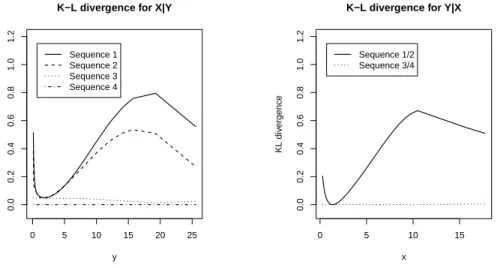
We calculated the Kullback-Leibler divergence curves for all regression models based on the complete data, or the “Before Deletion” data. The plots in Figure 2.1 show the divergence curves for each model from the four sets corresponding to fX|Y

and fY|X. From Sequence 1 to Sequence 4, the model fitting is gradually improved

since the divergence curve is gradually closer to 0 for both conditional densities, and both divergence curves reach 0 for Sequence 4 as it uses a validly specified model

set. In particular, the Kullback-Leibler divergence between fitted m32 and the true conditional density Z Z log fX|Y(x|y) m32(x|y,θˆBD2 ) fXY(x, y)dxdy

from Sequence 3 is uniformly close to 0 (less than 0.05 given any y); Furthermore, in the neighborhood of θ₁∗, Z Z _∂logm 31(y|x, θ1) ∂θ1 h fY(y)m32(x|y,θˆBD2 )−fXY(x, y) i dxdy =o(1),

which means that fitted m31 (based on Y and imputed X from fitted m32) is also

close to the true distribution. Therefore, we regard m31 and m32 in Sequence 3 as a

well-fitting model sequence for (X, Y). The choice of these 4 sequences enables us to demonstrate that better fitting model sequences yield better imputation results regardless of model compatibility/incompatibility.

0 5 10 15 20 25 0.0 0.2 0.4 0.6 0.8 1.0 1.2

K−L divergence for X|Y

y KL div ergence Sequence 1 Sequence 2 Sequence 3 Sequence 4 0 5 10 15 0.0 0.2 0.4 0.6 0.8 1.0 1.2

K−L divergence for Y|X

x

KL div

ergence

Sequence 1/2 Sequence 3/4

Figure 2.1: Kullback-Leibler divergence curves between fitted regression models and true condi-tional densities of four sets of models for Example 2.4.

All these models are reasonably well fitting models and cover the span of incom-patibility that includes: (1) Possibly compatible sequence with separable marginal

parameters; (2) Possibly compatible sequence with non-separable marginal parame-ters; (3) Incompatible model sequence; and, finally, (4) Specified possibly compatible sequence with non-separable marginal parameters; Model sequence 3 is a very well-fitting but incompatible model sequence that can be chosen by imputers because of the skewness of the residuals. The last model sequence may not likely to be cho-sen in practice but it is from the true conditional distributions; This enables us to demonstrate that convergence can be reached for all types of model sequences.

We also want to illustrate a gradual improvement strategy for practical purpose through the first two algorithms: after conducting proper transformation such as Box-Cox transformation determined by the available data, imputers may start with a simple linear regression model sequence for the transformed data, and then gradually improve the linear model sequence by fine-tuning it based on further model diagnosis, such as adding extra nonlinear terms in the models; in our example, residual plots suggest that the extra non-linear term 1/y in model m22 improves model fitting

compared to model m12.

Our primary evaluation criterion for imputation performance is the maximum of absolute difference between the empirical joint distribution based on the “Before Deletion” data and the “After Imputation” data at iterationT:

Fb n,T M I(x, y)−Fb_BDn (x, y) _∞.

We evaluated this conservative distance measure at T=5, 10, 20, 100, 500 and 1000 iterations. We fixed the number of imputations at 100. For each of 500 data sets, the distance measure was computed to form a function of n and T.

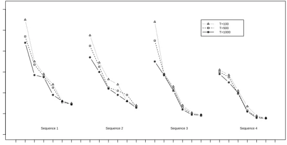
The averaged empirical joint distribution differences over 500 data sets from all four algorithms with different sample sizes and T=100, 500 and 1000 iterations are summarized in Figure 2.2. All sequences using fewer iterations T=5, 10, 20 yielded larger differences with similar patterns, so we excluded them in the figure to achieve

better visual effect. The simulation results show that as T and n increases, the empirical joint distribution difference from each sequence stabilizes. When T and n are sufficiently large, the average (SD) of the differences between the before deletion and multiple imputation empirical distributions is 0.0288 (0.006) for Sequence 1; 0.0257 (0.006) for Sequence 2; 0.0188 (0.005) for Sequence 3 and 0.0155 (0.004) for Sequence 4. The empirical joint distribution difference decreases from Sequence 1 to Sequence 4, indicating that as the model fitting is improved, the performance is improved as well. Both incompatible but better fitting sets from Sequences 2 and 3 outperform the possibly compatible set with separable marginal parameters from Sequence 1. The simulation study suggests that the validity of the inferences depends more on the reasonableness of the model fit rather than the model compatibility.

0.00 0.02 0.04 0.06 0.08 0.10 0.12 sample size

Max Absolute Diff

erence Betw

een Imputed/Bef

ore Deletion Empir

ical Distr ib utions 50 100 200 500 ₁₀₀₀ 10000 50 100 200 500 ₁₀₀₀ 10000 50 100 200 500 ₁₀₀₀ 10000 50 100 200 500 ₁₀₀₀ 10000 T=100 T=500 T=1000

Sequence 1 Sequence 2 Sequence 3 Sequence 4

Figure 2.2: Maximum of absolute difference between empirical distributions based on multiply im-puted data and before deletion data,

Fb n,T

M I(x, y)−Fb_BDn (x, y)

_∞, from four imputation algorithms plotted as a function of sample size n=50, 100, 200, 500, 1000 and 10000 and the number of iterationsT= 100,500,1000 for Example 2.4.

2.5 Non-ignorable Missing Data Mechanism

The sequential regression approach discussed earlier in this chapter ignores the missing data mechanism and, hence, we limited our discussion to missing at random mechanism. Nonetheless, it may be important to know what would happen if a user were to use this approach when the mechanism is nonignorable.

• When data are missing not at random, the meaning of the validly specified model is not clear and the modeling task will be different than the usual se-quential regression approach. Theorem 2.1 clearly requires a validly specified model and we believe that with a nonignorable missing data mechanism, the sequential regression model ignoring the missing data mechanism cannot be a validly specified model.

• It should be noted that even if one were to formulate a joint distribution for the variables, ignore the missing data mechanism when actually it is nonignorable then the algorithm (for example, Gibbs Sampling) may converge to something that has very little meaning. This may be true also for SRMI. We investigate further through a simulation study described later.

• Theorem 2.2 on the other hand is valid, as the construction and proof of Theo-rem 2.2 do not rely on missing data mechanism but depend only on the separable marginal parameter property of the target joint distribution.

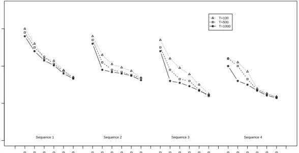
To investigate further, we extended our simulation study in section 2.4 by chang-ing only the misschang-ing data mechanism. We divided data into two equal random groups. In the first group, y is fully observed and the probability of x being ob-served is pr(x is observed|y) = [1 + exp(15 + 0.1y−5x)]−1; In the second group, x is fully observed and the probability of y being observed is pr(y is observed | x) =

[1 + exp(12−6y+ 0.1x)]−1. This results in about 45% of xvalues and 35% of the y values to be missing. Both xand y are missing Not at Random. Figure 2.3 shows a plot of the maximum difference between before deletion and after imputation empiri-cal CDFs; while the difference measure still converges for all algorithms as the sample size and number of iterations increase, none of the difference measures is close to 0, indicating biased imputation results due to ignoring the missing data mechanism.

0.00

0.05

0.10

0.15

Simulations for Data With Values Not Missing at Random

sample size

Max Absolute Diff

erence Betw

een Imputed/Bef

ore Deletion Empir

ical Distr ib utions 50 100 200 500 1000 10000 50 100 200 500 1000 10000 50 100 200 500 1000 10000 50 100 200 500 1000 10000 T=100 T=500 T=1000

Sequence 1 Sequence 2 Sequence 3 Sequence 4

Figure 2.3: Maximum of absolute difference between empirical distributions based on multiply im-puted data and before deletion data,

Fb n,T M I(x, y)−Fb_BDn (x, y)

∞, from four imputation

algorithms plotted as a function of sample sizen=50, 100, 200, 500, 1000 and 10000 and the number of iterationsT = 100,500,1000 when the data are not missing at random in Example 2.4.

2.6 Multivariate Missing Data

The appeal of sequential regression is the ability to handle missing values in complex multivariate data structure. The sequential regression imputation approach for the p-dimensional data Y1, . . . , Yp, assumesmi(yi |y[−i], θi), and θ

(t)

based on Yi,obs and Y

(t)

[−i]. Although the imputation procedure is similar to bivariate

algorithms, complications arise due to complex missingness patterns.

Consider the situation with three variables, (Y1, Y2, Y3), with all possible item

missing data patterns. The estimate θ(₁t) of θ1 in m1(Y1 | Y2, Y3, θ1) is obtained

by regressing the observed values of Y1 on the corresponding subset of Y2 and Y3.

The predictor subset consists of (Y2, Y3) in four missingness groups: 1. both are

observed, 2 & 3: one is observed and the other is imputed, and 4: both are imputed. The predictor variables in the four groups are generally distributed differently, and then each group plays a different role in estimating θ(₁t). For a data set with p variables, there are 2p−1 possible missingness groups, including the complete cases Ycc. It is difficult to establish results in generality given the complexity of the joint

distribution of the predictors.

2.6.1 Single Variable Missingness

We consider single variable missingness pattern where there is at most one variable missing in any record. There are up top+1 missingness groups, and we denoteR=i for subjects with Yi missing and R= 0 for the fully observed group.

During the estimation of each regression model, the subset of Y_[−(t)_i] form up to p patterns, and the log-likelihood is

li(θi |Yi,obs, Y (t) [−i]) =li(θi |Ycc) + X j<i li(θi |Y[−j], Y (t) j ) + X j>i li(θi |Y[−j], Y (t−1) j ). If there is no missingness inYj,li(θi |Y[−j], Y (t)

j ) is absorbed intoli(θi |Ycc), therefore

we assume for simplicity that there is missingness in each variable. The parameter estimate θ_i(t) is obtained by solving the score equation

si(θi |Yi,obs, Y_[−(t)_i]) =si(θi |Ycc) + X j<i si(θi |Y[−j], Yj(t)) + X j>i si(θi |Y[−j], Y(t −1) j ) = 0.

Based on θ_i(t), Yi,mis is drawn from mi(Yi,mis | Y[−i],obs, θ

(t)

i ), where Y[−i],obs are fully

observed. We now show that in terms of convergence properties, sequential regression imputation algorithms for multivariate missing data with single variable missingness are similar to those for bivariate missing data, and conclusions in Section 2.3 can be extended. The following theorems are a generalization of Theorems 2.1 and 2.2 for the bivariate case.

Theorem 2.3. Suppose p-dimensional data follow a joint population distribu-tion f(y1, . . . , yp | ψ) with conditional densities {fi(yi | y[−i], ψi), i = 1, . . . , p}.

If the sequential regression imputation algorithm uses a weakly incompatible model sequence{mi(yi |y[−i], θi), i= 1, . . . , p}and satisfies the regularity

condi-tions for the differentiation/integration and the mean/variance of the score func-tions, then fori= 1, . . . , p,mi(yi |y[−i], θ

(t)

i )→fi(yi |y[−i], ψi), asn, m, t→ ∞.

Theorem 2.4. Suppose that the sequential regression imputation algorithm uses possibly compatible models{mi(yi |y[−i], θi), i= 1, . . . , p}and satisfies the

regularity conditions in Theorem 2.3, withθ∈ΘC as the subspace of Θ1×Θ2×

. . . xΘp where p(y1, . . . , yp |θ1, . . . , θp, θ ∈ ΘC) defines the joint distribution. If

the model sequence has separable marginal parameters and (θ∗₁, . . . , θ_p∗)∈ΘC is

the maximum likelihood estimate of (θ1, . . . , θp) based on the joint likelihood,

then mi(yi |y[−i], θ (t)

i )→p(yi |y[−i], θi∗), as n, m, t→ ∞.

Proof of both theorems are extensions of proofs for Theorems 2.1 and 2.2 and these are included in the supplementary material available on the website or from the authors.

2.7 Discussion

Multiple imputation through specifications of a sequence of conditional regression models is a convenient approach for handling complex data structures with differ-ent types of variables. Several software packages have been developed to implemdiffer-ent this approach and are being used in several substantive analyses in various disci-plines. However, theoretical properties of this method have not been systematically investigated. One key question is whether using a set of incompatible conditional distributions leads to convergence or stability of the infinite imputation completed data statistics. Recently, Li, Yu and Rubin (LYR) (2012) have raised caution using some theoretical examples. However, these examples differ from the usual sequential regression setup in many ways. We address these examples in light of the results given in this chapter.

Example 1 in LYR uses a deterministic set of incompatible conditional normal distributions (that is, the same parameters are used across all updating iterations) to show that different ordering of updating the iterations leads to different results. However, the sequential regression does not use deterministic set of conditionals but the parameters themselves are updated at each iteration. We conducted a simu-lation study with the complete data (before deletion data sets) of size n = 7000 on 3 variables, Y = (Y1, Y2, Y3), from a multivariate normal distribution with mean

(−1,0,1) and the covariance matrix (1−ρ)I3+ρJ3 where I3 is an identity matrix

of order 3 and J3 is a 3 ×3 matrix of ones. Some values were deleted such that

all possible 7 patterns are represented in the after deletion data. The number of subjects in each pattern was 1000. The missing values were imputed using the fol-lowing weakly incompatible models: (1) Y1|Y2, Y3 ∼ N(αo +α1Y2 +α2Y3, σ21); (2)

Y2|Y1, Y3 ∼ N(βo +β1Y1 +β2Y3, σ22); and (3) Y3|Y1, Y2 ∼ N(γo+γ1Y1 +γ2Y2, σ32).

The imputations were carried out in three different orders (Y1, Y2, Y3), (Y2, Y1, Y3)

and (Y3, Y1, Y2). The number of imputations was fixed at 100 and the number of

iterations considered were T = 20,50,200,500 and 1000. Our results show that the multiple imputation estimates of the mean and the covariance matrix are unbiased for each of the three orders in which imputations were carried out. This shows that order of the imputation may be irrelevant and incompatibility does not result in bias as long as each conditional model is validly specified.

Example 3 in LYR uses a grossly misspecified model sequence in the imputation for a bivariate normal data. When the imputation models are misspecified or the missing data mechanism is not ignorable, it is difficult to assess whether it is the property of the method or the effect of misspecification. Even in this case, consider the following situation: suppose the data are missing at random and the imputer uses the model Y1|Y2 ∼N(αo+α1Y2, σ12) and Y2|Y1 ∼N(βo+β1Y1+β2Y12, σ22) then

Theorem 2.1 applies and the sequential regression imputation algorithm results in the consistent estimator of the joint distribution of (Y1, Y2). The key, therefore, is not

to fix the parameters across the iterations but revise the estimates based on updating of the imputed values. Thus asymptotically, the observed data tend to pull towards the consistent model when the joint distribution is embedded in the parameter space of the conditional distributions. Thus, our investigations suggest that the sequential regression approach may yield valid results if the conditional distributions fit the data well even though they may not be compatible with any joint distribution.

There are number of limitations in this study. The investigation was restricted to a missing data pattern with any subject missing values on at most one variable. This was mainly to restrict the number of missing data patterns to a manageable