Bootstrap LM tests for higher-order spatial effects in spatial linear regression models

Singapore Management University Singapore Management University

Institutional Knowledge at Singapore Management University

Institutional Knowledge at Singapore Management University

Research Collection School Of Economics School of Economics

1-2018

Bootstrap LM tests for higher-order spatial effects in spatial linear

Bootstrap LM tests for higher-order spatial effects in spatial linear

regression models

regression models

Zhenlin YANG

Singapore Management University, [email protected]

Follow this and additional works at: https://ink.library.smu.edu.sg/soe_research

Part of the Econometrics Commons

Citation Citation

YANG, Zhenlin. Bootstrap LM tests for higher-order spatial effects in spatial linear regression models. (2018). Empirical Economics. 55, (1), 35-68. Research Collection School Of Economics.

Available at:

Available at: https://ink.library.smu.edu.sg/soe_research/2336

This Journal Article is brought to you for free and open access by the School of Economics at Institutional Knowledge at Singapore Management University. It has been accepted for inclusion in Research Collection School Of Economics by an authorized administrator of Institutional Knowledge at Singapore Management University. For

Bootstrap LM Tests for Higher Order Spatial Effects

in Spatial Linear Regression Models

Zhenlin Yang∗

School of Economics, Singapore Management University Email: [email protected]

December 22, 2017

Abstract

This paper first extends the methodology of Yang (2015, J. of Econometrics 185, 33-59) to allow for non-normality and/or unknown heteroskedasticity in obtaining asymptotically refined critical values for the LM-type tests through bootstrap. Bootstrap refinements in critical values require the LM test statistics to be asymptotically pivotal under the null hypothesis, and for this we provide a set of general methods for constructing LM and robust LM tests. We then give detailed treatments for two general higher order spatial linear regression models: namely the SARAR(p, q) model and the MESS(p, q) model, by providing a complete set of non-normality robust LM and bootstrap LM tests for higher order spatial effects, and a complete set of LM and bootstrap LM tests robust against both unknown heteroskedasticity and non-normality. Monte Carlo experiments are run, and results show an excellent performance of the bootstrap LM-type tests.

Key Words: Asymptotic pivot; Bootstrap; Heteroskedasticity; LM test; Spatial lag; Spatial error; Matrix exponential; Wild bootstrap; Bootstrap critical values. JEL classifications: C12, C15, C18, C21.

1. Introduction

Since the birth of spatial econometrics in the early 1970s, various forms of spatial inter-actions have been incorporated into a linear regression model to give what is called in the paper the spatial linear regression (SLR) model with one or more of the following: spatial lag dependence (SLD), spatial error dependence (SED), and spatial Durbin effect (SDE). The SLD effect can be in either the spatial autoregressive (SAR) form or the matrix exponential spatial specification (MESS), and theSEDeffect can be in the same form as theSLDeffect and, in addition, it can be in the form of the spatial moving average (SMA) or the spatial error components (SEC). These give a rich class of SLR model of ‘order’ one.1 Recently, theory and

∗

I am grateful to Singapore Management University for financial support under Grant C244/MSS16E003. I thank Badi Baltagi for the invitation, and Harry Kelejian and two referees for the helpful comments.

1

See Anselin (1988b) and Anselin and Bera (1998) for various specifications of the SLR models withSLD,

applications have advanced the SLR model to contain various spatial effects of order higher than one, e.g., the SLR model with a SAR response of order p and a SAR error of order q, referred to in the literature asSARAR(p, q); the SLR model with apth orderMESS in response and aqth order MESS in error, referred to in the literature asMESS(p, q).2

Evidently, it is desirable to have simple tools that help practitioners choose an appropriate SLR model. The LM test has been an important tool for identifying the existence of various types of spatial effects in a linear regression model as it requires only the estimation of the null model, often an ordinary linear regression model. However, the usual LM tests may not have a satisfactory finite sample performance, and various refined LM tests for SLR models involving SED,SLD, orSEChave been introduced, such as the LM tests based on standardization (Yang, 2010; Baltagi and Yang, 2013a), the LM tests based on Edgeworth correction (Robinson and Rossi, 2014, 2015a,b), and the LM tests based on bootstrap critical values (Yang, 2015; Jin and Lee, 2015). Standardization improves the finite sample performance of a two-sided test, but it may not be able to do so for a one-sided test as the spatial dependence drives the finite sample null distribution of the test statistic skewed, and more so with a denser spatial weights matrix (Yang, 2015). Edgeworth correction method is rather limited (Horowitz, 1994; Hall and Horowitz, 1996), and it may be feasible only when the null model is an ordinary least square (OLS) regression, due to the complications in deriving the Edgeworth expansion. In contrast, bootstrap critical values are very easy to obtain, and more importantly they give a second-order approximation to the finite sample critical values of the LM test statistic if it is asymptotically pivotal when the null hypothesis is true. The method is rather general as well, as it works in the same way when the null model containsnonlinear parameters(parameters need to be estimated through numerical optimization) as when the null model is an OLS regression, except that it incurs some additional computation. See Section 4 for details.

Furthermore, the usual LM tests are derived under Gaussian likelihoods and the assump-tion that the errors are independent and identically distributed (iid). Neither assumpassump-tion can be realistic, in particular the assumption of homoskedasticity (see Anselin, 1988b). Regular LM tests forSED(including Moran’sI test given in Moran (1950)) and/or SLDare shown to be robust against distributional misspecification (Baltagi and Yang, 2013a), but the regular LM test forSEC is not (Yang, 2010). In general, the regular LM test are not robust against unknown heteroskedasticity. Born and Breitung (2011) gave a set of heteroskedasticity and non-normality robust LM tests for the SLR models withSED and/orSLD. Baltagi and Yang (2013b) followed up with a set of ‘standardized’ heteroskedasticity and non-normality robust LM tests which are shown to have much improved finite sample property.3 However, these tests are again very likely to suffer from the problem of finite sample size-distortion for one-sided tests. The LM tests referring to the ‘one-one-sided’ bootstrap critical values may offer finite

2

The basic motivation for a higher order SLR model is that spatial units may subject to different types of interactions (e.g., geographical distance, social relationship, peer effects). See Badinger and Egger (2011) and Elhorst et al. (2012) forSARAR(p, q) and the supplement file to Debarsy et al. (2015) forMESS(p, q).

3

sample refinements, but this issue is not formally examined though it was raised in Yang (2015). Also, for certain SLR models such as the SLR model with SEC and the SLR model withMESS, neither LM tests nor bootstrap LM (BLM) tests that are robust to unknown het-eroskedasticity and non-normality are available. An SLR model specification with both SLD and SECdoes not seem to have appeared in the literature, and so are the corresponding LM and BLM tests. Finally, most of the LM tests available in the literature test the spatial effects of ‘order one’, and the LM tests for higher order spatial effects, in particular the BLM tests, are not available. This paper will fill in some of these gaps. We will focus on the LM-type tests that are either robust against nonnormality or robust against both non-normality and unknown heteroskedasticity. It is seen that once the general principles are clear and strictly followed, the actual implementations of the BLM tests are quite straightforward.

The rest of the paper is organized as follows. Section 2 presents the bootstrap method, discusses its validity, and presents some simple examples. Section 3 outlines the general principles for constructing LM and robust LM tests. Section 4 presents LM and BLM tests and their robust versions for the SARAR(p, q) model, and Section 5 presents the same set of tests for the MESS(p, q) model. Section 6 presents some Monte Carlo results, showing an excellent performance of the BLM tests. Section 7 concludes the paper with discussions.

2. Bootstrap LM Tests: General Methods and Validity

2.1. The models

All the SLR models discussed in the introduction, except the models with SEC, fall into the following general model specification:

An(λ)Yn=Xnβ+un, Bn(ρ)un=εn, (2.1)

whereYn is ann×1 vector of response values,Xn is ann×kmatrix that contain the values

of exogenous regressors and may contain some spatial Durbin terms, An(λ) ≡ An(W`, λ) is

an n×n matrix inducing SLDof order p inSAR or MESS form andBn(ρ) ≡Bn(We, ρ) is an n×nmatrix inducing SEDof order q inSAR orSMAorMESS form,W`={W`1· · ·, W`p} and

We = {We1,· · · , Weq} with W`j and Wej being the given n×n spatial weights matrices, β

is ak×1 vector of regression coefficients, λis ap×1 vector of spatial lag parameters,ρ is a

q×1 vector of spatial error parameters, andεn is ann×1 vector of idiosyncratic errors, iid

with mean 0 and varianceσ2_ε, or independent but not identically distributed (inid) with mean zero and variances hiσε2, i = 1,· · ·, n where {hi} represent the unknown heteroskedasticity.

Most of the tests in the literature correspond to the models with p = 1 and q = 1. In this paper, they are extended for testing the higher-order spatial effects.

For example, for an SLR model withpth orderSLDandqth orderSEDboth in the autore-gressiveform, we haveAn(λ) =In−Pp_j=1λjW`j andBn(ρ) =In−P_jq₌₁ρjWej whereInis an

n×nidentity matrix, leading to theSARAR(p, q) model. For an SLR model withpth orderMESS in response andqth order MESS in error, or the MESS(p,q) model, An(λ) = exp(Pp_j=1λjW`j)

andBn(ρ) = exp(Pqj=1ρjWej) as in the literature, or the proposed forms in Section 5 to

over-come the difficulty in finding the partial derivatives. For an SLR model withSDE, it is typical that Xn = (Xn, W1nX1n) where X1n is a submatrix of Xn, excluding at least the columns

corresponding to the intercept and dummy variables to avoid multicollinearity problem. An alternative model specification is to replace Bn(ρ)εn on the right-hand side of (2.1)

byWevn+εn, to give an SLR model withSLDof order p(in SARorMESS form) and SEC:

An(λ)Yn=Xnβ+Wevn+εn, (2.2)

where the spatial error component Wevn is independent ofεn with the elements of vn being

iid of mean zero and variance σ2_v (see Kelejian and Robinson, 1995). These types of model specifications have not been considered in the literature and a full study of them is interesting but beyond the scope of this paper. In this paper, we will concentrate on Model (2.1) with eitherSARAR(p, q) or MESS(p, q), and offer discussions relating to Model (2.2).

2.2. Bootstrap methods and their validity

To give a general procedure for bootstrapping the critical values of an LM test, let θbe the parameter vector that corresponds to the null model, and ϕ be the parameter vector of which the value is specified by the null hypothesis as zero. As we are mainly interested in tests for spatial effects, theϕ vector would include all or some of the spatial parameters, which areλandρunder Model (2.1), andλandσ2

v under Model (2.2); and theθvector would

always include β and σ2_ε, and may contain some spatial parameters. The most interesting tests would be ones of which the null hypotheses specify that all the spatial parameters in the model are zero, as in these cases, the null models are simply the ordinary least squares (OLS) regression models. Some tests of model reduction are also interesting, e.g., from SARAR(p, q) toSARAR(1,1). The Durbin terms act as some additional regressors and hence are treated together with the regular regressors although they may create an additional problem of parameter identification (see Elhorst, 2014, and Lee and Yu, 2016).

Consider the following general hypothesis:

H0 :ϕ= 0,

and let the corresponding LM test be

LMn≡LMn(Yn,Xn,Wn),

whereWn= (W`,We). Note that under Model (2.2), we consider the cases whereϕcontains σ_v2 so that under H0 the spatial error componentvn vanishes. Thus, the above set-up covers

both models. Clearly, the statistic LMn is an explicit function of (Yn,Xn,Wn) when the

spatial parameters whose estimates at the null are implicit functions of (Yn,Xn,Wn).

Case I: iid errors. Consider first the case of iid errors and let F be the cumulative distribution function (CDF) ofεni, theith element ofεn. Write the null models as

Yn=h(Xn,Wn; θ; εn). (2.3)

Let ˆθn be an estimate of θ, consistent whether or not the null hypothesis is true. Let ˆεn

be an estimate of εn centered to have mean zero, and ˆFn be the corresponding empirical

distribution function (EDF), also ‘consistent’ whether or not the null hypothesis is true.4 For the bootstrap critical values to achieve second-order approximation to the finite sam-ple critical values of an LM test, Yang (2015) laid out the following fundamental princisam-ples:

(i) the bootstrap data generating process (DGP) must be set up so that it is able to mimic the null model, (ii) the LM statistic must be asymptotically pivotal under the null, (iii) the estimates of the nuisance parameters, to be used as parameters in the bootstrap DGP, must be consistent whether or not the null hypothesis is true, (iv) the EDF of the residuals consistently estimates the error distribution whether or not the null hypothesis is true, and (v) calculation of the bootstrapped values of the LM statistic is done under the null hypothesis.

Note that the null model is determined by the pair (θ,F), so is the finite sample null distribution of LMn. We are interested in the finite sample CDF Gn(θ,F) of LMn under H0

(or LMn|H0), in particular the finite sample critical valuescn(α;θ,F) of LMn|H0, 0< α <1. With the fundamental principles given above, the bootstrap DGP must be set up as follows:

Y_n∗=h(Xn,Wn; ˆθn; ε∗n), {ε ∗ ni}

iid

∼ Fˆ_n, (2.4)

where ˆθn acts as parameters and ˆFn acts as error distribution, called, respectively, the boot-strap parameters and the bootstrap error distribution, so that it is able to mimic the real world null DGP given in (2.3). With the bootstrap data (Y_n∗,Xn,Wn) so generated through

(2.4), the bootstrap analogue of LMn is given as LM∗n ≡LMn(Yn∗,Xn,Wn). It follows that

the bootstrap CDF of LM_n∗ must have the formGn(ˆθn,Fˆn), identical in structure toGn(θ,F),

and that the bootstrap critical value must be cn(α; ˆθn,Fˆn), identical in form to cn(α;θ,F).

These can be seen more clearly from the following identical structures:

LMn|H0 ≡LMn(Yn,Xn,Wn) = LMn(h(Xn,Wn;θ;εn),Xn,Wn)≡LMn(Xn,Wn; θ; εn), LM∗_n≡LMn(Yn∗,Xn,Wn) = LMn(h(Xn,Wn; ˆθn;ε∗n),Xn,Wn)≡LMn(Xn,Wn; ˆθn;ε∗n).

Under certain conditionscn(α; ˆθn,Fˆn) gives a second-order approximation to cn(α;θ,F).

However, in real applications, the true bootstrap critical value is infeasible as it is numeri-cally too demanding to exhaust all the possible bootstrap samples. The following algorithm summarizes the steps leading to approximate bootstrap critical values.

4

A natural choice for the pair (ˆθn,Fˆn) in connection with the LM tests would be the quasi maximum likelihood estimates (QMLEs) of the full model containingθandϕ, but it is not restricted to the full QMLEs. In fact, any pair of√n-consistent estimates, such as GMM estimates, of the full model can be used.

Algorithm 2.1. (iid bootstrap)

(a) Draw a random sampleε∗_n from Fˆn;

(b) Compute Y_n∗ =h(Xn,Wn; ˆθn; ε∗n), to obtain the bootstrap data{Yn∗,Xn,Wn}; (c) Estimate the null model based on{Y_n∗,Xn,Wn}, and then compute a bootstrapped value

LM∗_n of LMn;

(d) Repeat (a)-(c) B times to obtain bootstrap values{LMb_n}B

b=1 of LMn, and theα-quantile

cB_n(α; ˆθn,Fˆn) of {LMbn}Bb=1 gives a bootstrap approximation to cn(α;θ,F).

The validity of the above bootstrap procedure needs to be addressed. First, as B can be made arbitrarily large, the approximation from cB_n(α; ˆθn,Fˆn) to cn(α; ˆθn,Fˆn) can be made

arbitrarily accurate, and hence such an approximation will be ignored in the following dis-cussions. What is left is to argue that cn(α; ˆθn,Fˆn)−cn(α;θ,F) =Op(n−1). The following

assumptions are adapted from Yang (2015).

Assumption A1. The errors{εni} are iid (0, σε2) with CDF F, known or unknown.

Assumption A2. The LM-type statisticLMnis asymptotically pivotal underH0, whether

or not F is correctly specified.

Assumption A3. (ˆθn,Fˆn) is

√

n-consistent for (θ,F) whether or not H0 is true, and

whether or notF is correctly specified.

Assumption A4. For (ϑ,F)∈ Nθ,F, a neighborhood of (θ,F), the null CDF Gn(·, ϑ,F)

converges weakly to a limit null CDF G(·, ϑ,F) as n increases, and admits the following

asymptotic expansion uniformly int and locally uniformly for (ϑ, F)∈ Nθ,F:

G_n(t, ϑ,F) =G(t, ϑ,F) +n− 1

2g(t, ϑ,_F) +O(n−1), (2.5)

where G(·, ϑ,F) is differentiable and strictly monotone over its support, and g(t, ϑ,F) is a

functional of (t, ϑ,F) differentiable in(ϑ,F).

Assumption A1 is standard and the existence of higher-order moments is implied by the assumptions that follow. Assumption A2 suggests that the limiting CDF of LMn|H0 is G(·), free from (θ,F). This is generally true ifF is known or correctly specified, but may not be true ifF is unknown or misspecified. In the latter case, some modification on the usual LM statistic is necessary to make it robust against distributional misspecification. Assumption A3 unifies the different cases considered in Yang (2015). It was stressed in Yang (2015) that the bootstrap parameters ˆθn must be a consistent estimator of the population parametersθ

in the null model whether or not the null hypothesis is true, as in real applications one does not know whether or not H0 is true. This is an important point, but did not

seem to have been emphasized in the literature until Yang (2015), and instead, the literature seemed pointed to a contrary (see, e.g., van Giersbergen and Kiviet, 2002; Godfrey, 2009, Ch. 3; MacKinnon, 2002). Clearly, from (2.3) and (2.4) one sees that Y_n∗ would not be able to mimic Yn when H0 is false but the restricted (inconsistent) estimate ˜θn is used in (2.4),

unless the null distribution of the test statistic does not depend on θ as in certain special cases such as (2.14) and (2.18). See Yang (2015) for detailed discussions on this. Assumption A4 is a general technical assumption given in Yang (2015) by adapting a similar condition given Beran (1988). In an important special case where the test statistic is asymptotically

N(0,1), the asymptotic expansion (2.5) reduces to the following Edgeworth expansion:

Gn(t, θ,F) = Φ(t) +n−

1

2φ(t)p(t, θ,F) +O(n−1), (2.6) where Φ andφare, respectively, the CDF and pdf ofN(0,1),p(t, θ,F) =−k1,2+1₆k3,1(1−t2),

and k1,2 and k3,1 are the n-free polynomials defined in the following expansion for the jth

cumulantκj,n ≡κj,n(θ,F) of LMn|H0 (Hall, 1992, Sec. 2.3):

κj,n =n− j−2

2 (k_j,1+n−1k_j,2+n−2k_j,3+· · ·). (2.7)

Obviously,k1,1 = 0 andk2,1 = 1 in connection with the facts thatκ1,n →0 andκ2,n →1, as n→ ∞. Developing an asymptotic or Edgeworth expansion for a general LM statistic is by no means an easy task. Fortunately, the bootstrap method (discussed in this paper) itself does not require the derivation of asymptotic or Edgeworth expansions. It is just that (quoting Hall, 1992, p. v): “Methods based on Edgeworth expansion can help explain the performance of bootstrap methods, and on the other hand, the bootstrap provides strong motivation for reexamining the theory of Edgeworth expansion.”

Yang (2015) developed Edgeworth expansions specific to the SLR models with SED, or SLD or SEC, for the purpose of formal justifications on the validity of the iid bootstrap method given above. Jin and Lee (2015) developed Edgeworth expansion under normality and Edgeworth expansions for martingales under nonnormal errors for the CDF of a test statistic that can be approximated by linear quadratic forms. Robinson and Rossi (2014, 2015a,b) derived Edgeworth expansions for the pure SAR model and the SLR model with SEDunder normality, for analytically correcting the distributions of the LM statistics.

Proposition 2.1. Under Assumptions A1-A4, the bootstrap critical value given in Algo-rithm 2.1 is such that cn(α; ˆθn,Fˆn)−cn(α;θ,F) =O(n−1); in contrast c(α)−cn(α;θ,F) = O(n−12) where c(α) is the corresponding critical value of the limiting distribution G(·).

Proof. Only a sketch of the proof is given here in the general form. Details corresponding to some particular models can be found in Yang (2015). Under Assumption A2, the limiting distribution of LMn|H0 must be such thatG(t, θ,F) =G(t), and under Assumptions A3 and A4, that of LM∗_nmust beG(t,θˆn,Fˆn) =G(t) as well based on the triangular-array convergence

(see Beran, 1988). Thus, under Assumptions A1-A4, the CDF of LMn|H0 and the bootstrap CDF of LM∗_n possess the following stochastic expansions:

Gn(t, θ,F) = G(t) +n− 1 2g(t, θ,F) +O(n−1), (2.8) G_n(t,θˆn,Fˆn) = G(t) +n− 1 2g(t,θˆ_n,Fˆ_n) +O_p(n−1). (2.9)

Taking the difference, we have

G_n(t,θˆn,Fˆn)− Gn(t, θ,F) =n−

1

2[g(t,θˆ_n,Fˆ_n)−g(t, θ,F)] +O_p(n−1) =O_p(n−1), where the last equality follows from the√nconsistency of (ˆθn,Fˆn) and the differentiability

ofg(t, ϑ,F) in (ϑ,F)∈ Nθ,F.

Remark 2.1. From the proof of Proposition 2.1, it is clear that without√n-consistency of (ˆθn,Fˆn), the term g(t,θˆn,Fˆn)− Gn(t, θ,F) would not be Op(n−

1

2), and the second-order approximation ofGn(t,θˆn,Fˆn) to Gn(t, θ,F) would not be achieved.

Case II: inid errors. Consider again the real world null DGP:Yn=h(Xn,Wn; θ; εn)

defined in (2.3). When{εni}are inid with mean zero and varianceshiσ2ε, Algorithm 2.1 based

on the bootstrap DGP (2.4) is no longer valid, as the iid draws lost the heteroskedasticity structure. Based on the fundamental principles laid out below (2.3), a valid bootstrap DGP able to capture the unknown heteroskedasticity must be that (i) ˆθn is a consistent estimator

of θ whether or not H0 is true and is robust against non-normality (NN) and unknown

heteroskedasticity (UH), (ii) the estimated residuals {εˆni} are consistent with {εni}, i.e.

ˆ

εni = εni +op(1), whether or not H0 is true, and (iii) bootstrap samples based on the

estimated residuals are able to mimic (consistently estimate) εn. Clearly, a valid choice of

ˆ

θn and ˆεni is from the NN-UH robust estimation of the full model (see, e.g., Kelejian and

Prucha (2010), Lin and Lee (2010), and Liu and Yang (2015). The modified bootstrap DGP, thewild bootstrap, takes the form:

Y_n∗ =h(Xn,Wn; ˆθn; ε∗n), εˆ ∗

ni= ˆεnivi, (2.10)

where{vi}ni=1 areniid draws from a distributionH(·) with mean 0 and higher-order moments

all 1, independent ofεni.5 See, e.g., Wu (1986), Liu (1988), Mammen (1993), Godfrey (2007),

and Davidson and Flachaire (2008), for an account on wild bootstrap.

To facilitate the discussion on the validity of the wild bootstrap procedure, denote the NN-UH robust LM-type statistic by LMRn, and the bootstrap analogue of LMRn|H0 by LMR

∗ n. Clearly, LMRn|H0 ≡LMRn(Xn,Wn; θ; εn), and LMR ∗ n≡LMR ∗ n(Xn,Wn; ˆθn; ε∗n). Assume the CDF ofh− 1 2

i εni isF(·) with higher-order momentsµ={µ3, µ4, . . .}. Thus, εni has CDF

F(·/√hi), and the moments µir =h_ir/2µr, r = 1,2, . . .. The bootstrap distribution of ˆε∗ni is

H(·/εˆni), which is H(·/εˆni) if ˆεni >0; 1− H(·/εˆni) o.w. Its moments are ˆµ∗_ir = E∗(ˆεr_nivr_i) =

ˆ

εr_niE(v_ir). Define the product measures Fn =Qni=1F(·/ √

hi) and ˆHn =Qni=1H(·/εˆni). Let

Gn(·, θ,Fn) be the finite sample CDF of LMRn|H0 and cn(α;θ,Fn) be its αth quantile; let G_n(·,θˆn,Hˆn) be the bootstrap CDF of LMR∗n and cn(α; ˆθn,Hˆn) be its αth quantile.

5

In fact, such a distribution does not exist but, often, being able to match up to 3rd or 4th moments suffices (see Mammen, 1993, and Remark 2.2 below). The well-knownRademacherdistribution (vi=±1 with equal probabilities) has all the odd moments being 0, and all the even moments being 1. This is an ideal distribution when the original errors are symmetrically distributed. Another popular choice is Mammen’s (1993) two-point distribution: P{vi =−(

√

5−1)/2}= (√5 + 1)/(2√5), andP{vi= ( √

5 + 1)/2}= (√5−1)/(2√5), which gives E(vi) = 0, E(vi2) = 1, and E(v3i) = 1, but E(vi4) = 2.

A feasible bootstrap procedure for obtainingcn(α; ˆθn,Hn) is summarized below.

Algorithm 2.2. (wild bootstrap)

(a) Draw a random sample{vi}ni=1 from the chosenH, to give εn∗ ={εˆnivi}ni=1;

(b) Compute Y_n∗ =h(Xn,Wn; ˆθn; ε∗n), to obtain the bootstrap data{Yn∗,Xn,Wn}; (c) Perform an NN-UH robust estimation of the null model based on {Y_n∗,Xn,Wn}, and

then compute a bootstrapped valueLMR∗_n of LMRn;

(d) Repeat (a)-(c) B times to obtain bootstrap values {LMRb_n}B

b=1 of LMRn, and the α

-quantilecB_n(α; ˆθn,Hˆn) of {LMRbn}Bb=1 gives a bootstrap approximation to cn(α;θ,Fn).

Assumption B1. The errors {εni} are inid (0, σε2hi) where hi >0 and _n1

Pn

i=1hi = 1. The CDF ofh−

1 2

i εni isF, with necessary higher-order momentsµ={µ3, µ4,· · · }being finite.

Assumption B2. The LM-type statistic, LMRn, is asymptotically pivotal underH0, and

is robust against misspecification inF and unknown heteroskedasticity.

Assumption B3. Whether or notH0 is true, (i)θˆn is

√

n-consistent forθ and is robust against misspecification inF and unknown heteroskedasticity, and (ii) εˆni =εni+Op(n−1/2).

Assumptions B1-B3 extends Assumptions A1-A3 to cater the unknown heteroskedasticity. These extensions seem straightforward. Assumption B1 essentially assumes thatεni=h

1 2

i eni

and{eni}are iid as in Liu and Prucha (2016). With Assumptions B2 and B3, it is reasonable

to assume that G_n(·,θˆn,Hˆn) converges to the same limit as does Gn(·, θ,Fn). No doubt,

proving the existence of Edgeworth/asymptotic expansions for the case of inid errors is even more challenging than the already challenging case of iid errors in spatial models. To simplify the discussions, we put up the following higher-level assumptions compared with Assumption A4 for the case of iid errors, and details may be learnt based on, e.g., (2.20) and (2.21).

Assumption B4. The null CDFG_n(·, θ,Fn) and the bootstrap CDF Gn(·,θˆn,Hˆn) admit the following asymptotic expansions:

Gn(t, θ,Fn) = G(t) +n− 1 2g(t, θ,F_n) +O(n−1), (2.11) G_n(t,θˆn,Hˆn) = G(t) +n− 1 2g(t,θˆ_n,Hˆ_n) +O(n−1), (2.12)

where g(t, θ,Fn) is a functional of (t, θ,Fn) differentiable in (θ,Fn).

Proposition 2.2. Under Assumptions B1-B3, the bootstrap critical value given in Algo-rithm 2.2 is such thatcn(α; ˆθn,Hˆn)−cn(α;θ,Fn) =O(n−1); in contrastc(α)−cn(α;θ,Fn) = O(n−12) where c(α) is the corresponding critical value of the limiting distribution G(·).

Proof. Parallel to the proof of Proposition 2.1.

Remark 2.2. As in the case of iid errors, an Edgeworth expansion similar to (2.6) can be obtained for a univariate test, from which one sees that g(t, θ,Fn) depends only on the

leading terms in the expansions for the first three cumulants of LMRn|H0. Furthermore, it can be shown that in a number of special tests, g(t, θ,Fn) depends on Fn only through the

first three moments ofεni as in Yang (2015) for the case of iid errors. This is important as

it says that as long as the wild bootstrap is able to capture the first three moments ofεni, a

full second-order refinement on the critical values can be achieved.

2.3. Examples

To help appreciating the general methods given above, we present several simple tests concerning theSARAR(1,1)effects, and concerning SECeffect.

Example 2.1. Joint and conditional tests for SARAR(1,1). To test for the existence of 1st order SLDor 1st order SED or both in a linear regression model, the three LM tests due to Burridge (1980) for the first one and Anselin (1988a,b) are given as follows:

LMSLD = n q ˜ Jn+Kn`` ˜ ε0<sub>n</sub>W`Yn ˜ ε0<sub>n</sub>ε˜n , (2.13) LMSED = n p Kee n ˜ ε0<sub>n</sub>Weε˜n ˜ ε0 nε˜n , (2.14) LMSARAR = (˜ε0<sub>n</sub>W`Yn)2Knee−2(˜ε0nW`Yn)(˜ε0nWeε˜n)Kn`e+ (˜ε0nWeε˜n)2(Jn+Kn``) ˜ σ4 n[JnKnee+Kn``Knee−(Kn`e)2] ,(2.15)

where ˜εn is the vector of OLS residuals from regressing Yn on Xn, ˜Jn = ˜σn−2η˜n0Mnη˜n, ˜ηn = W`Xnβ˜n, ˜βnand ˜σ2nare the null estimates of β and σ2,Mn=In−Xn(X0nXn)−1X0n,Kn`` =

tr[(W`+W`0)W`],Knee= tr[(We+We0)We], andKn`e= tr[(W`+W`0)We]. WhenW`=We≡Wn

is assumed in (2.15),K_n``=K_nee=K_n`e ≡Kn and the test simplifies to

LM0_SARAR= (˜ε 0 nWnYn−ε˜0nWnε˜n)2 ˜ σ2 nη˜0nMnη˜n +(˜ε 0 nWnε˜n)2 ˜ σ4 nKn . (2.16)

These three tests can easily be shown to be robust against nonnormality by verifying the (asymptotic) equivalence in variance-covariance matrices; see Section 4 for details under the general SARAR(p, q) model. However, their finite sample performance when referred to the asymptotic critical values (ACVs) can be poor. Use of bootstrap critical values (BCVs) can greatly reduce the size distortion. As the three tests correspond to the same null model, the bootstrap DGP has the same form: Y_n∗ =Xnβˆn+ε∗n, where {ε∗ni} aren random draws

from centeredunrestricted residuals{εˆni}, i.e, the residuals calculated from the estimation of

the ‘full’ model, being respectivelySARAR(0,1),SARAR(1,0), andSARAR(1,1), and ˆβn is the

unrestricted estimate ofβ. Clearly, ˆσ_n2 does not play a role in generating the bootstrap data. To obtain the BCVs of the LM tests given above, take for example the test LM0_SARARgiven in (2.16). Based on the bootstrap data (Y_n∗,Xn, Wn), one estimates the null model and then

calculates the test statistic to obtain its bootstrap value or its bootstrap analogue:

LM0_SARAR∗ = (˜ε ∗0 nWnYn∗−ε˜∗0nWnε˜∗n)2 ˜ σ∗2 n η˜∗0nMnη˜n∗ +(˜ε ∗0 nWnε˜∗n)2 ˜ σ∗4 n Kn , (2.17)

where ˜η_n∗ = ˜σ∗−1

n WnXnβ˜n∗, ˜βn∗ and ˜σn∗2 are the bootstrap estimates of β and σ2, i.e., from

regressing Y_n∗ on Xn, and ˜ε∗n = Yn∗ −Xnβ˜n∗ = Mnε∗n. Repeated draws from {εˆni} give

sequences of bootstrap values of LM0_SARAR∗ , and their quantiles give the BCVs for LM0_SARAR, as in Algorithm (2.1). Similarly, one obtains the BCVs for LMSLD, LMSED, and LMSARAR. The results of Yang (2015) imply that the BCVs for the above tests give a second-order approximation to the finite sample critical values (FCVs) of these tests. In contrast the asymptotic critical values (ACVs) only approximate the FCVs to the first order.6

Example 2.2. Testing for the existence of SEC. Consider the SLR-SEC model: Yn =

Xnβ+Wnvn+εn. The test forSECamounts to test H0:σν2= 0, or λ=σν2/σ2 = 0. An LM

test is given in Anselin (2001), and a robust LM test is given in Yang (2010):

LMRSEC= n q Kn†+ ˜κ4na0nan ˜ ε0_nHn†ε˜n ˜ ε0_nε˜n , (2.18) whereHn†=WnWn0 −n−k1 tr(WnWn0Mn)In,Kn†= 2tr(A2n), an= diagv(An), An=MnHn†Mn, ˜

κ4n is the 4th cumulant of ˜σn−1ε˜n, and ˜σ2nis the estimate ofσ2 underH0. The null model and

the bootstrap DGP are again OLS regressions. The bootstrap analogue of (2.18) is thus:

LMR∗_SEC= q n Kn†+ ˜κ∗_4na0nan ˜ ε∗0_nHn†ε˜∗n ˜ ε∗0 nε˜∗n , (2.19)

where ˜ε∗_n is the vector of residuals from regressing Y_n∗ on Xn, ˜κ∗4n is the 4th cumulant of

˜

σ_n∗−1ε˜∗_n, and ˜σ∗_n2 is the bootstrap estimate ofσ2 from the same regression. Yang (2015) show that the BCVs give second-order approximations to the FCVs.

Example 2.3. Heteroskedasticity and non-normality robust LM tests for SARAR(1,1).

While the LM tests given in (2.13)-(2.15) are robust against non-normality of the error dis-tribution, they are not robust against unknown heteroskedasticity. Their robust versions (against both non-normality and heteroskedasticity) are given in Born and Breitung (2011):

LMRSLD = ˜ ε0_nW`Yn (˜ε20 n ξ˜12n) 1 2 , (2.20) LMRSED = ˜ ε0<sub>n</sub>Weε˜n (˜ε20 n ξ˜22n) 1 2 , (2.21) LMRSARAR = ˜ ε0<sub>n</sub>W`Yn ˜ ε0_nWeε˜n !0 ˜ ε_n20ξ˜2_1n, ε˜_n20( ˜ξ1nξ˜2n) ∼, ε˜2_n0ξ˜₂2_n !−1 ˜ ε0_nW`Yn ˜ ε0_nWeε˜n ! , (2.22) 6 As_n1Pn

i=1εˆni= 0,{ˆεni}are automatically centered. Apparently, LM

∗

SEDis invariant of ˆβnand hence any estimate ofβcan be used in the bootstrap DGP. The estimate of the scale parameterσalso does not play a role and is absorbed in ˆεn andε∗n. However, the use of the unrestricted residuals is necessary as the ‘finite sample’ distribution of LMSED|He

0depends on the third moment ofεniand only with the unrestricted residuals

the third moment of ˆFnis √

where ˜ξ1n= (W`u0+W`l)˜εn+Mnη˜n, ˜ξ2n= (Weu0+Wel)˜εn,Aun andAln denote the upper and

lower triangular matrices of a matrixAn, ‘’ denotes the Hadamard product,a2=aafor

a vectora, and ˜εn and ˜ηnare as in (2.13)-(2.15). Baltagi and Yang (2013b) show that these

tests referring ACVs can perform very poorly and present standardized versions of them. The three tests have the same null DGP: Yn = Xnβ +εn. The wild bootstrap DGP

is Y_n∗ = Xnβˆn+ε∗n, ε∗n = ˆεnvn, where vn is an n-vector of iid draws from an auxiliary

distribution with mean zero and higher moments 1, completely independent of original data. With the bootstrap data (Y_n∗,Xn, Wn), one computes ˜ε∗n, ˜η∗n, and hence ˜ξ1∗n and ˜ξ2∗n, giving

bootstrap values of the test statistics and hence the BCVs.

3. Construction of LM and Robust LM Tests

In this section, we outline the general procedures for constructing LM tests, robust LM tests against nonnormality, and robust LM tests against both nonnormality and unknown heteroskedasticity. Then, in the subsequent sections, we apply these general procedures to introduce LM/BLM and robust LM/BLM tests, respectively, for the SARAR(p, q) model and theMESS(p, q) model. We endeavor to present the results in a practical manner so the applied researchers can easily apply these BLM tests.

Recall: θ represents parameter vector in the null model, ϕ the additional vector of pa-rameters appeared in the full model, and the null hypothesis specifiesϕ= 0. Letψ= (θ0, ϕ0)0 and ψ0 (θ0 and ϕ0) be the true value of ψ (θ and ϕ), Sn(ψ) the score vector based on the

normality assumption onεn, and Σn(ψ0) =−E[_∂ψ∂0Sn(ψ0)]. Corresponding to θ and ϕ,

de-note the subvectors ofSn(ψ) bySn,θ(θ, ϕ) andSn,ϕ(θ, ϕ), and the submatrices of Σn(ψ) by

Σn,θθ(θ, ϕ), Σn,ϕϕ(θ, ϕ) and Σn,θϕ(θ, ϕ). The LM testof H0:ϕ= 0 takes the form:

LMn= ˜Sn,ϕ0 Σ˜−n1

ϕϕS˜n,ϕ, (3.1)

with its limiting null distribution beingχ2_dim(ϕ), where ˜Sn,ϕ=Sn,ϕ(˜θn,0), ˜Σn= Σn(˜θn,0), ˜θn

is the MLE of the null model, and (·)ϕϕ denotes theϕ-ϕblock of the corresponding matrix.

By the definition of Σn(ψ0), it is clear that ˜Σn can simply be−_∂ψ∂0Sn(˜θn,0).

LM test robust against non-normality (NN). Let Γn(ψ0) = Var[Sn(ψ0)], with

sub-matrices Γn,θθ(θ, ϕ), Γn,ϕϕ(θ, ϕ) and Γn,θϕ(θ, ϕ). By Taylor expansion,

1 √ nSn,ϕ(˜θn,0) = 1 √ nSn,ϕ(θ0,0)− 1 √ nΠn(θ0)Sn,θ(θ0,0) +op(1), (3.2)

where Πn(θ0) = Σn,ϕθ(θ0,0)Σ−_n,θθ1 (θ0,0). It follows that Var[√1_nSn,ϕ(˜θn,0)] = _n1

Γn,ϕϕ(θ0,0)−

Γn,ϕθ(θ0,0)Π0n(θ0)−Π0n(θ0)Γn,θϕ(θ0,0) + Πn(θ0)Γn,θθ(θ0,0)Π0n(θ0)

+o(1). An NN-robust LM test, with its limiting null distribution beingχ2

dim(ϕ), takes the form:

LMN_n0 = ˜S_n,ϕ0 Γ˜n,ϕϕ−2˜Γn,ϕθΠ˜0n+ ˜ΠnΓ˜n,θθΠ˜0n

−1_˜

where ˜Sn,ϕ =Sn,ϕ(˜θn,0), ˜Γn,ϕϕ, ˜Γn,ϕθ and ˜Γn,θθ are the submatrices of Γn(˜θn,0), and ˜Πn =

Πn(˜θn). Clearly, when {εni} are iid normal, Γn(ψ0) = Σn(ψ0) (information matrix equality,

or IME) and LMNn reduces to LMn. When{εni}are iid but non-normal, the IME does not

hold and the explicit expression of Γn(θ0,0) is required in order to implement LMN0n. It is

typical that Γn(θ0,0) involves higher-order moments of the model errors which are estimated

based on the null residuals defined by ˜θn.

Analternative wayto estimate Γ(θ0,0) is via theouter-product-of-martingale-difference

(OPMD) (Baltagi and Yang, 2013b; Yang, 2017). If Sn(θ0,0) has a martingale difference

(MD) representation: Sn(θ0,0) =Pni=1gni(θ0), where {gni(θ0)} form an MD sequence, then

Var[Sn(θ0,0)] =Pn_i=1Var[gni(θ0)] =Pn_i=1E[gni(θ0)g_ni0 (θ0)]. Hence, Pn_i=1g˜ni˜g_ni0 , the sum of

the estimated OPMDs, thus gives a consistent estimate of Var[Sn(θ0,0)] in the sense that 1 n[ Pn i=1˜gnig˜ 0 ni−Var[Sn(θ0,0)] p

−→0, where ˜gni =gni(˜θn). Replacing ˜Γn,ϕϕ, ˜Γn,ϕθ and ˜Γn,θθ

in (3.3) by the submatrices ofPn

i=1˜gnig˜ni0 , we obtain an OPMD form of NN-robust LM test:

LMNn= ˜S0n,ϕ

Pn

i=1(˜gni,ϕ−Π˜ng˜ni,θ)(˜gni,ϕ−Π˜n˜gni,θ)0

−1_˜

Sn,ϕ. (3.4)

Equivalently, (3.4) can be obtained as follows. By (3.2) and the MD representationSn(θ0,0) = Pn

i=1gni(θ0),Sn,θ(˜θn,0) has the following asymptotic MD representation: 1 √ nSn,ϕ(˜θn,0) = 1 √ n Pn i=1[gni,ϕ−Πn(θ0)gni,θ] +op(1), (3.5)

where{gni,ϕ−Πn(θ0)gni,θ}form an MD sequence with (g0ni,θ, g 0 ni,ϕ) 0 _=g ni ≡gni(θ0). Thus, Var[√1 nSn,ϕ(˜θn,0)]= 1 n Pn

i=1E[(gni,ϕ−Πn(θ0)gni,θ)(gni,ϕ−Πn(θ0)gni,θ)0]+o(1), leading to (3.4).

The advantages of using the OPMD estimate of Γn(θ0,0) are: (i) it avoids the

analyti-cal expression of Γn(ψ0) containing higher order moments, and (ii) it is also robust against

unknown heteroskedasticity (UH) besides being robust against NN. These are crucial in de-veloping LM tests that are both NN and UH robust, as seen below. With these, an OPMD alternative to the LM test (3.1) can be easily developed.

LM test robust against NN and UH. Neither LMn nor LMNn (or LMN0n) is robust

against UH in model errors. To derive an LM-type test that is UH-robust, adjust Sn(ψ)

so that the adjusted score vector S_n◦(ψ) is such that E[S_n◦(ψ0)|H0] = 0 or 1 nS ◦ n(ψ0)|H0 p → 0

as n → ∞ under UH. Let ˜θ_n◦ = arg{S_n,θ◦ (θ,0) = 0}, the UH-robust estimator of the null model. Let Σ◦_n(ψ0) = −E[_∂ψ∂0S_n◦(ψ0)] and Γ◦n(ψ0) = Var[Sn◦(ψ0)], partitioned similarly as

Σn(ψ0) and Γn(ψ0). IfSn◦(θ0,0) has a martingale difference (MD) representation: Sn◦(θ0,0) = Pn

i=1g

◦

ni(θ0) where {g ◦

ni(θ0)} form an MD sequence, then, similar to Sn,θ(˜θn,0) in (3.5), S_n,θ◦ (˜θ◦_n,0) has the following asymptotic MD representation:

1 √ nSn,ϕ(˜θ ◦ n,0) = √1n Pn i=1[gni,ϕ(θ0)−Π◦n(θ0)gni,θ(θ0)] +op(1),

Σ◦_n,ϕθ(θ0,0)Σ

◦₋₁

n,θθ(θ0,0). An OPMD-based and NNUH-robust LM test takes a similar form:

LMNHn= ˜Sn,ϕ◦0

Pn

i=1(˜gni,ϕ◦ −Π˜◦n˜gni,θ◦ )(˜gni,ϕ◦ −Π˜◦n˜g◦ni,θ)0

−1_˜

S◦_n,ϕ, (3.6)

where the tildequantities are the estimates at H0 of the corresponding quantities. Clearly,

the key in developing the UH-robust LM tests is to find the adjusted quasi score function

S_n◦(θ0,0) that is UH-robust, and hence the UH-robust estimate ˜θ◦n= arg{Sn,θ◦ (θ0,0) = 0}.

Notation: To proceed with details for each model, some general notation would be helpful: (i) for a matrixCn,Cns =Cn+Cn0; (ii) for a square matrixCn, its upper triangular,

lower triangular and diagonal matrices are denoted, respectively, by C_nu, C_nl and C_nd such that Cn = Cnu+Cnl +Cnd, and its diagonal elements are denoted by Cn,ii; (iii) {aj} forms

a row vector if a0_js are scalars, or a matrix if a0_js are column vectors, and {bij} denotes a

matrix formed by the elementsbij; (iv) 0m is an m×1 vector of zeros; (v) a quantity with

atildedenotes the restricted (under the null) QMLE of that quantity; and (vi) a parametric quantity, e.g., Σn(ψ), will be denoted as Σn when ψ=ψ0, shall no confusion arises.

4. BLM and Robust BLM Tests for

SARAR

(

p, q

)

Model

Consider theSARAR(p, q) model given in Section 2.1: An(λ)Yn=Xnβ+un, Bn(ρ)un=εn,

where An(λ) =In−

Pp

j=1λjW`j and Bn(ρ) =In−

Pq

j=1ρjWej,W` ={W`1· · · , W`p} and

We={We1,· · · , Weq}. The following hypotheses are of primary interest, forp, q≥2:

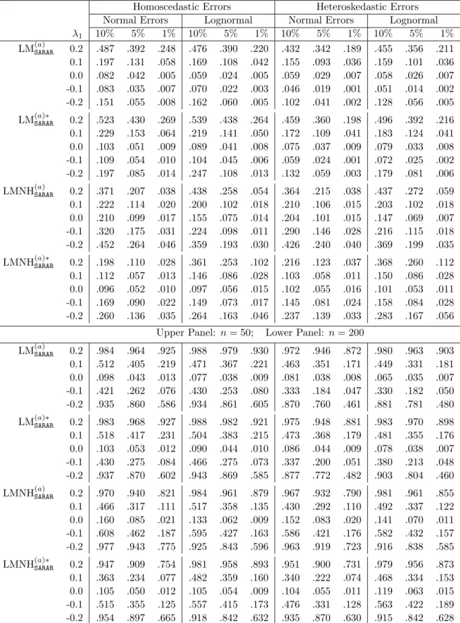
(a) H₀a: λ= 0 and ρ= 0, in SARAR(p, q); (b)H₀b: λ2 =· · ·=λp = 0 and ρ2 =· · ·=ρq = 0, inSARAR(p, q); (c) H₀c: λ= 0, inSARAR(p, q); (d) H₀d: ρ= 0, in SARAR(p, q); (e) H₀e: λ= 0, inSARAR(p,0); (f) H₀f: ρ= 0, in SARAR(0, q).

The generic set-up given in Section 3, where the null hypothesis is denoted byH0:ϕ= 0 and

the parameter vector in the reduced model byθ, facilitates the general discussion. These tests are all tests of model reduction (from a larger SLR model down to a smaller SLR model). Other tests of model reduction may also be of interest, e.g., tests ofSARAR(1,0) vsSARAR(p,0), SARAR(1,0) vs SARAR(p, q), SARAR(0,1) vs SARAR(0, q), SARAR(0,1) vs SARAR(p, q), etc., and can all be handled by the general method introduced below.

Likelihood, score and information matrix. The Gaussian loglikelihood for the SARAR(p, q) model is`n(ψ) =−n₂ln(2πσ2)+ln|An(λ)|+ln|Bn(ρ)|−_2σ12ε

0

n(β, δ)εn(β, δ), where εn(β, δ) = Bn(ρ)[An(λ)Yn−Xnβ] and δ = (λ0, ρ0)0. Maximizing `n(ψ) gives the maximum

likelihood estimator (MLE) ˆψnofψwhen the errors are normally distributed, otherwise quasi

can be easily obtained to give the restricted (Q)MLE ˜θn of the parameter vector θ. Both

ˆ

ψn and ˜θn are robust against non-normality. The ˆθn component of ˆψn will be used in the

bootstrap procedure as it is√n-consistent whether or not the null is true.7 The score function,Sn(ψ) = _∂ψ∂ `n(ψ), has the form:

Sn(ψ) =                1 σ2X0_nB_n0(ρ)εn(β, δ), 1 2σ4ε 0 n(β, δ)εn(β, δ)− ₂n_σ2, 1 σ2ε0n(β, δ)Bn(ρ)W`jYn−tr(Cjn(λ)), j= 1,· · · , p, 1 σ2ε0_n(β, δ)Djn(ρ)εn(β, δ)−tr(Djn(ρ)), j= 1,· · ·, q, (4.1)

whereCjn(λ) =W`jA−n1(λ) andDjn(λ) =WejB−n1(ρ). The information matrix has the form:

Σn(ψ0) =        1 σ2 0 X0_nB_n0BnXn, 0, ₁ σ2 0 X0_nB_n0ηjn , 0 ∼, ₂n_σ2 0, ₁ σ02tr(Cjn) , ₁ σ20tr(Djn) ∼, ∼, ₁ σ2 0 η0_jnηj0_n+ tr( ¯C_jnC¯s j0_n) , tr( ¯CjnDjs0_n) ∼, ∼, ∼, tr(DjnDjs0_n)        , (4.2) whereηjn≡ηjn(β0, δ0) =Bn(ρ0)Cjn(λ0)Xnβ0 and ¯Cjn≡C¯jn(δ0) =BnCjnBn−1, j= 1· · ·, p.

Recall the{·} notation is defined before the start of this section. Finally, the concentrated score ofδ afterβ and σ2 being concentrated out has the form:

˜ Sn,δ(δ) =    1 ˜ σ2 n(δ)ε˜ 0 n(δ)Bn(ρ)W`jYn−tr(Cjn(λ)), j= 1,· · · , p, 1 ˜ σ2 n(δ)ε˜ 0 n(δ)Djn(ρ)˜εn(δ)−tr(Djn(ρ)), j= 1,· · · , q, (4.3)

where ˜ε0_n(δ) =ε_n0 ( ˜βn(δ), δ), and ˜βn(δ) and ˜σ2n(δ) are the QMLEs ofβ and σ2 at a givenδ.

LM and BLM tests. The tests in (a)-(d) are of the same nature as each corresponds to a test of model reduction from the fullSARAR(p, q), p, q≥2 model down to a model with fewer spatial terms. Thus, they take the general form given in (3.1), or the following reduced form given by Liu and Yang (2017):

LMSARAR(δ) = ˜Sn,δ0 (δ) ˜ Jn(δ) +Kn``(δ), Kn`e(δ) K<sub>n</sub>`e0(δ), K_nee(δ) !−1 ˜ Sn,δ(δ), (4.4) where ˜Sn,δ(δ) is in (4.3); ˜Jn(δ) = _σ˜21 n(δ) ˜ η_jn0 (δ)Mn(ρ)˜ηj0_n(δ) p×p, ˜ηjn(δ) = ηjn( ˜βn(δ), δ),

7_{For the asymptotic properties of the QMLEs under homoskedasticity, see Lee (2004) forSARAR(1,0) model,}

Jin and Lee (2013) forSARAR(1,1) model, and Liu and Yang (2017) forSARAR(p, q) model. For the asymptotic properties of the QMLEs under unknown heteroskedasticity, see Liu and Yang (2015) forSARAR(1,0) model, and Liu and Yang (2017) forSARAR(p, q) model. For GMM estimation of theSARAR(p, q) model under homoskedas-ticity, see Lee and Liu (2010). For GMM estimation of theSARAR(p, q) model under heteroskedasticity, see Lin and Lee (2010), Kelejian and Prucha (2010), and Badinger and Egger (2011).

j= 1,· · ·, p,Mn(ρ) =In−Xn(ρ)[X0n(ρ)Xn(ρ)]−1X0n(ρ),Xn(ρ) =Bn(ρ)Xn; and K_n``(δ) = tr( ¯CjnC¯js0_n)−2tr( ¯Cjn)tr( ¯Cj0_n) p×p, K_n`e(δ) = tr( ¯CjnDsj0_n)−2tr( ¯C_jn)tr(D_j0_n) p×q, K_nee(δ) = tr(DjnDsj0_n)−2tr(D_jn)tr(D_j0_n) q×q.

With the general expression (4.4), the LM test statistics for (a)-(d) are obtained by setting

δ = 0 for (a), (˜λ1n,00p−1,ρ˜1n,00q−1)0 for (b), (00p,ρ˜0n) for (c), and (˜λ0n,00q) for (d), where the tilded parameters are the constrained QMLEs of the corresponding parameters under the respective null hypothesis. For easy reference, the resulted statistics are denoted, respectively, by LM(_SARARa) , LM(_SARARb) , LM(_SARARc) , and LM(_SARARd) .

Of particular interest is LM(_SARARa) for testing H₀a: λ= 0 and ρ= 0, which takes the form:

LM(_SARARa) = 1 ˜ σ4 n ˜ ε0_nW`Yn ˜ ε0<sub>n</sub>Weε˜n !0 ˜ Jn+Kn``, Kn`e K_n`e0, K<sub>n</sub>ee !−1 ˜ ε0<sub>n</sub>W`Yn ˜ ε0_nWeε˜n ! , (4.5)

where ˜ε0_nW`Yn denotes (˜ε0nW`1Yn,· · ·,ε˜0nW`pYn)0, ˜ε0nWeε˜ndenotes (˜ε0nWe1ε˜n,· · · ,ε˜0nWeqε˜n)0,

˜

εn, ˜βn and ˜σn2 are from OLS regression of Yn on Xn, ˜Jn=

₁ ˜ σ2 nη˜ 0 jnMnη˜j0_n , ˜η_jn=W<sub>`j</sub>X<sub>n</sub>β˜<sub>n</sub>, K<sub>n</sub>`` =tr(W`jW`js0) , K<sub>n</sub>`e = tr(W`jWejs0) ,K_nee = tr(WejWejs0) , andM_n =M_n(0). The

LM test LM(_SARARa) can easily be simplified to give LM tests for H₀(e) and H₀f: LM(_SLDe) = σ˜−_n4(˜ε_n0 W`Yn)0 J˜n+Kn`` −1 (˜ε0<sub>n</sub>W`Yn), (4.6) LM(_SEDf) = σ˜−_n4(˜ε0_nWeε˜n)0 Knee −1 (˜ε0_nWeε˜n). (4.7)

These tests generalize the tests given in Example 2.1, and can be shown to be NN-robust by verifying that the ‘variance’ in (3.3) is (asymptotically) equivalent to ˜Σn,ϕϕ−Σ˜n,ϕθΣ˜−n,θθ1 Σ˜n,θϕ.

Liu and Yang (2017) show that the asymptotic null distributions of the tests for the hypotheses in (a)-(f) are chi-square with degrees of freedom being, respectively,p+q,p+q−2,

p, q, p and q. However, the finite sample performance of these tests when referring to the chi-square critical values can be poor, similar to the tests for SARAR(1,1) model given in (2.13)-(2.15). They went on to derive the finite sample improved versions of these tests by re-standardizing the concentrated scores. However, as seen from their work, the method of re-standardization can be complicated when the concentrated scores involve estimates of nonlinear spatial parameters such as the cases (b)-(d), besides the issues related to one-sided tests. In this paper, we demonstrate how the bootstrap provide refined approximation to the finite sample critical values, leading to tests with a second-order accuracy in size. As discussed in Section 2, for bootstrap to achieve second-order accuracy, the test statistic has to be an asymptotic pivotal under the null. In this sense, one can use the simplest form of test statistic without going through the complicated process of restandardization. Furthermore, in cases that tests are univariate and one-sided tests can be carried out, bootstrap method offers an additional advantage of being able to approximate the actual one-side critical values.

The bootstrap versions of the above tests can be obtained in a similar way as in Example 2.1. Let ˆβnbe the unrestricted QML estimate of β and ˆεn the unrestricted QMLE residuals.

The bootstrap DGP is Y_n∗ =Xnβˆn+ε∗n, where ε∗n is an n×1 vector of iid draws from the

EDF of ˆεni, taking the same form for all three tests but with ˆβn and ˆεn corresponding to

SARAR(p,0), SARAR(0, q), and SARAR(p, q), respectively. Taking the test LM(_SLDe) given in (4.6) for example, based on the bootstrap data (Y_n∗,Xn,W`), the bootstrap analogue of LMeSLD is LM(<sub>SLD</sub>e)∗ = ˜σ∗−<sub>n</sub> 4(˜ε∗0<sub>n</sub>W`Yn∗)0 J˜n∗ +Kn``

−1

(˜ε∗,0n W`Yn∗). Repeated samples from the EDF of ˆεn

give a sequence of bootstrap values for LMSLD, and hence the BCVs.

To demonstrate further how flexible the bootstrap method is, we use the test statis-tic LM(_SARARb) , obtained from (4.4) by replacing δ by ˜δn = (˜λ1n,00p−1,ρ˜1n,00q−1)0, for testing

SARAR(1,1) vs SARAR(p, q). In this case, θ = (β, σ2, λ1, ρ1)0, and ϕ = (λ2, . . . , λp, ρ2, . . . , ρq)

which is 0p+q−2 under the null. Let ˆθn be the MLE ofθand ˆεnbe the ML residuals from the

estimation of the fullSARAR(p, q) model, based on the original data. The bootstrap DGP is

Y_n∗ = (In−λˆ1nW`1)−1[Xnβˆn+ (In−ρˆ1nWe1)−1ε∗n], (4.8)

whereε∗_nis a vector ofniid draws from the EDF of ˆεn. Based on the bootstrap data from the

above DGP: (Y_n∗,Xn, W`1, We1), estimate the null model SARAR(1,1) to give the bootstrap

estimates ˜β_n∗,˜σ_n∗2, and ˜δ∗_n= (˜λ∗_1n,00_p−1,ρ˜∗_1n,00_q−1)0, and then compute the bootstrapped value:

LM(_SARARb)∗ = ˜S_n,δ0 (˜δ_n∗) ˜ Jn(˜δ∗n) +Kn``(˜δn∗), Kn`e(˜δn∗) K<sub>n</sub>`e0(˜δ_n∗), K_nee(˜δ∗_n) !−1 ˜ Sn,δ(˜δn∗), (4.9)

where ˜Sn,δ(δ) is given in (4.3) and other quantities are defined below (4.4). Repeat this

process B times to give a sequence of bootstrapped values of LM(_SARARb) under the null, and their sample quantiles give the bootstrap critical values.

NN-robust LM and BLM tests. To give LM and BLM tests that are generally robust against non-normality, we follow the OPMD method introduced in Section 3 as this method gives an NN-UH robust estimate of the variance of the score without the need of an analytical expression of it. Also this method is simple and the resulted test statistics are asymptotically pivotal at the null, which is all it is needed for BLM to achieve second-order accuracy.

Writing the element Bn(ρ)W`jYn in the quasi score function Sn(ψ) given in (4.1) as

¯

Cjn(δ)Yn(δ) whereYn(δ) =Bn(ρ)An(λ)Yn and noticing that Yn(δ0) =Xn(ρ0)β0+εn. Then,

at the true parameter valueψ0, we have, for the score vector given in (4.1),

Sn(ψ0) =                1 σ2 0 X0_nB_n0εn, 1 2σ4 0ε 0 nεn− ₂n_σ2 0, 1 σ2 0ε 0 nC¯jnεn+_σ12 0ε 0 nηjn−tr(Cjn), j= 1,· · ·, p, 1 σ2 0ε 0 nDjnεn−tr(Djn), j= 1,· · · , q. (4.10)

This leads immediately to an MD representation: Sn(ψ0) =Pni=1gni(ψ0), where gni(ψ0) =                1 σ2 0 xbiεni, 1 2σ4 0 (ε2_ni−σ2₀), 1 σ2 0

[εniξjn,i+ ¯Cjn,ii(ε2ni−σ20) +ηjn,iεni], j= 1,· · ·, p,

1

σ2 0

[εniζjn,i+Djn,ii(εni2 −σ20)], j= 1,· · · , q,

(4.11)

wherexbi is the ith column ofX0nBn0,ξjn= ( ¯Cjnu0 + ¯Cjnl )εn, and ζjn= (Du0jn+Dljn)εn.

Equipped with (4.2) and (4.11), and following general principles laid out by (3.4) and the discussions around it, we have the general form of NN-robust LM test:

LMN(_SARARm) = ˜S0_n,ϕ Pn

i=1(˜gni,ϕ−Π˜ng˜ni,θ)(˜gni,ϕ−Π˜n˜gni,θ)0

−1_˜

Sn,ϕ, (4.12)

wherem=a, b, c, d, e, f, giving the NN-robust tests for the six hypotheses listed above. The ˜

Πn can be either the plug-in estimate of Πn= Σn,ϕθΣ−_n,θθ1 based on Σn(ψ0) given in (4.2), or

the estimate based on the Hessian matrix, with θ and ϕ defined accordingly. For example, for testingHa

0 :δ = 0, we have θ= (β0, σ2)0 and ϕ=δ, Πn = Σn,ϕθΣ−_n,θθ1 has only non-zero

element at the upper-left corner block: η_jn0 Xn(ρ)[X0n(ρ)Xn(ρ)]−1 , and for tests in (e) and

(f), we haveθ= (β0, σ2)0, andδ =λfor (e) andρfor (f). Liu and Yang (2017) show that the null asymptotic distribution of LMN(_SARARm) is chi-square with degrees of freedom being dim(ϕ). Bootstrap critical values for the NN-robust LM tests are obtained in a similar manner. As discussed above, the parameter estimates maximizing the Gaussian likelihood of the SARAR models are robust against non-normality, the bootstrap DGPs take the same form as those for the case of the regular LM tests, e.g., (4.8) for testingSARAR(1,1) vsSARAR(p, q).

NNUH-robust LM and BLM tests. Under UH, i.e., εni ∼(0, σ02hi). From (4.10), it

is easy to see that theδ-component of E[Sn(ψ0)], involving {hi}, is not zero in general, and

that the probability limit of 1_nSn(ψ0) is not zero in general. Thus, the statistics developed

earlier would not converge to central chi-squares limiting distributions under the null, and inferences based on them would be misleading. Define

S_n◦(ψ) =                1 σ2X0nB0n(ρ)εn(β, δ), 1 2σ4ε0_n(β, δ)εn(β, δ)−₂n_σ2, 1 σ2ε 0 n(β, δ) ¯Cjn◦ (δ)Yn(δ), j= 1,· · · , p, 1 σ2ε0n(β, δ)Djn◦ (ρ)εn(β, δ), j= 1,· · · , q, (4.13)

where ¯C_jn◦ (δ) = ¯Cjn(δ)−diag( ¯Cjn(δ)) and D_jn◦ (δ) = Djn(δ)−diag(Djn(δ)). It is easy to

verify that, under UH, E[S_n◦(ψ0)] = 0 and _n1Sn◦(ψ0)

p

→0. Solving S_n◦(ψ) = 0 leads to NNUH-robust estimator ˆψ_n◦ forψ of the full model, and the ˆθ_n◦ component of ˆψ_n◦ will be used in the

bootstrap procedure discussed below. Similarly, solvingS_n,θ◦ (ψ) = 0 under H0 :ϕ= 0 gives

the restricted NNUH-robust estimator ˜θ◦_n ofθ. See Liu and Yang (2017) for details. Similarly, S_n◦(ψ0) has an MD representation: S◦n(ψ0) =Pni=1gni◦ (ψ0), where

g_ni◦ (ψ0) =                1 σ2 0xbiεni, 1 2σ4 0 (ε2_ni−σ₀2), 1 σ2 0 (εniξ◦_jn,i+η_jn,i◦ εni), j= 1,· · · , p, 1 σ2 0 εniζjn,i◦ , j= 1,· · · , q, (4.14)

wherexbiis as in (4.11),ξjn◦ = ( ¯Cjn◦u0+ ¯Cjn◦l)εn,ζjn◦ = (D◦u0jn +D◦ljn)εn, andηjn◦ = ¯Cjn◦ BnXnβ0.

WithS_n◦(ψ0) and its MD representation, letting ˜Π◦n= [∂θ∂0S_n,ϕ◦ (˜θ◦_n,0)][_∂θ∂0S_n,θ◦ (˜θ◦_n,0)]−1 be

a feasible estimate of Π◦_n = Σ◦_n,ϕθΣ◦_n,θθ−1, the LM tests fully robust against NN and UH take the general form as that given in (3.6):

LMNH(m)_SARAR= ˜S_n,ϕ◦0 Pn

i=1(˜gni,ϕ◦ −Π˜◦n˜gni,θ◦ )(˜gni,ϕ◦ −Π˜◦n˜g◦ni,θ)0

−1_˜

S◦_n,ϕ, (4.15) where ˜S_n,ϕ◦ =S◦_n,ϕ(˜θ◦_n,0), ˜g_ni,θ◦ and ˜g_ni,ϕ◦ are the subvectors ofg_ni◦ (˜θ◦_n,0), and m=a, b, c, d, e, f

corresponding to the six tests defined at the beginning of this section with relevant choice of θ and ϕ and the related quantities. Liu and Yang (2017) show that the null asymptotic distribution of LMNH(_SARARm) is chi-square with degrees of freedom being dim(ϕ).

We again use the case (b) with the test statistic LMNH(_SARARb) to provide details on the bootstrap procedures for obtaining refined approximations to the finite sample critical values of the test statistics. First, the test statistic LMHN(_SARARb) is obtained from (4.15) using ˜θ◦_n = ( ˜β_n◦0,σ˜_n◦2,˜λ◦_1n,ρ˜◦_1n)0. Based on the unrestricted estimates ˆθ◦_n = ( ˆβ_n◦0,σˆ_n◦2,λˆ◦_1n,ρˆ◦_1n)0 and the unrestricted residuals ˆε◦_n obtained from the UH-robust estimation of the full model, thewild

bootstrap DGP is set up as follows:

Y_n∗= (In−ˆλ◦1nW`1)−1[Xnβˆ◦n+ (In−ρˆ◦1nWe1)−1(ˆε◦nvn∗)], (4.16)

wherev_n∗ is a vector ofniid draws from a distribution as discussed in Section 2. Based on the bootstrap data from the above DGP: (Y_n∗,Xn, W`1, We1), estimate the null modelSARAR(1,1)

to give the bootstrap estimate ˜θ_n◦∗, and then compute the bootstrapped value: LMNH(b)_SARAR∗ = ˜S_n,ϕ◦∗0 Pn

i=1(˜gni,ϕ◦∗ −Π˜◦∗n ˜gni,θ◦∗ )(˜gni,ϕ◦∗ −Π˜◦∗n ˜g◦∗ni,θ)0

−1_˜

S◦∗_n,ϕ. (4.17) Repeat this processB times to give a sequence of bootstrapped values of LMNH(_SARARb) under the null, and their sample quantiles give the bootstrap critical values.8

8_{The usual plug-in estimate may not be feasible as the explicit expression of Σ}◦

n contains the unknown heteroskedasticity {hi} besides the regular parameters. It can easily be verified that the tests LMN(SARARa) , LMN(SARARe) , and LMN

(f)

5. BLM and Robust BLM Tests for

MESS

(

p, q

)

Model

Consider the SLR model with MESS(p, q) effect: An(λ)Yn = Xnβ +un, Bn(ρ)un = εn,

whereAn(λ) = exp(Pp_j=1λjW`j) and Bn(ρ) = exp(Pq_j=1ρjWej). Similar to the SARAR(p, q)

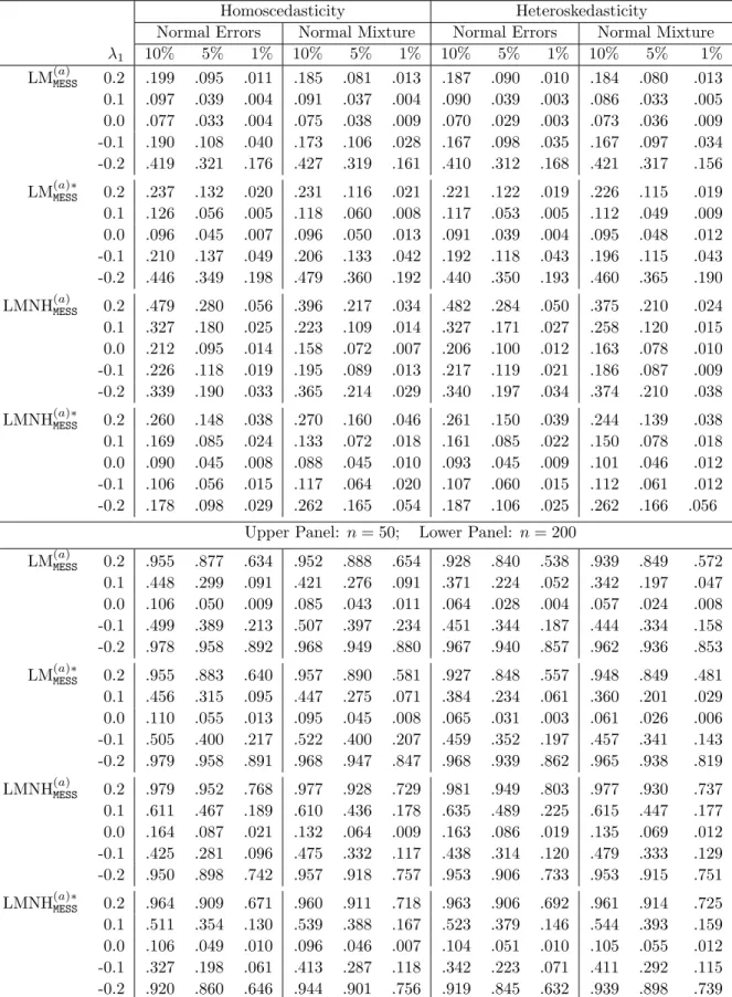
model, the following hypotheses are of primary interest: (a) H₀a: δ = 0, inMESS(p, q); (b)H₀b: λ2 =· · ·=λp = 0 and ρ2 =· · ·=ρq = 0, inMESS(p, q); (c) H₀c: λ= 0, inMESS(p, q); (d) H₀d: ρ= 0, in MESS(p, q); (e) He 0: λ= 0, inMESS(p,0); (f) H₀f: ρ= 0, in MESS(0, q).

Again, we use the notationδto denote (λ0, ρ0)0,θto denote the parameters in the null model, and ϕto denote the additional parameters in the full model which are specified by the null hypothesis to be zero. Other tests of model reduction concerning δ only can be treated in the same way, using the general methods introduced below.

We will proceed with the details on the construction of the LM and robust LM tests without providing detailed proofs of the results as they are largely implied by the asymptotic results in the supplement file to Debarsy et al. (2015), except the case of NNUH-robust LM tests, of which proofs require the central limit theorems for linear-quadratic form of Kelijian and Prucha (2001) and the weak law of large numbers of, e.g., Davidson (1994).

Likelihood, score and information matrix. The loglikelihood function of theMESS(p, q) model is`n(ψ) =−2_nln(2πσ2)−₂1_σ2ε0n(β, δ)εn(β, δ), whereεn(β, δ) =Bn(ρ)[An(λ)Yn−Xnβ].

Maximizing `n(ψ) gives the unrestricted MLE or QMLE ˆψn of ψ in the full model, and

maximizing the loglikelihood of the reduced model under the null gives the restricted MLE or QMLE ˜θn of θ. Note that, with MESS specifications, ln|An(λ)| = 0 and ln|Bn(ρ)| = 0.

Thus, the QML estimation of theMESS(p, q) model has a computational advantage over that of a SARAR(p, q) model as it avoids the repeated calculations of the determinants of the two matrices An(λ) and Bn(ρ) in the optimization process. Another advantage is that the

QM-LEs of theMESS(p,0) and MESS(0, q) models are robust against unknown heteroskedasticity, and the QMLEs of theMESS(p, q) model can be robust against unknown heteroskedasticity if

W`jWej0 =W<sub>ej</sub>0W<sub>`j</sub>, i.e., the two types of spatial weights matrices are commutative. These

can easily be seen by showing that the expectation of the score (given below) at the true pa-rameters values under UH are zero.9 _{To allow for more generality, we do not assumeW}

`j and Wej0 to be commutative, and propose a UH-robust QML-type estimators for the MESS(p, q)

model and use them in constructing the UH-robust bootstrap LM tests.

univariate tests given in (2.20) and (2.21) alone the lines of Yang (2015) for iid errors.

9

A further advantage of the QML estimation of theMESS(p, q) model is that its parameter space is unre-stricted, whereas the values of the parameters in theSARAR(p, q) must be restricted in a compact space which can be hard to find (Lee and Liu, 2010; Elhorst et al., 2012). Consistency and asymptotic normality of the QMLEs of the generalMESS(p, q) model are proved in the supplement file to Debarsy et al. (2015).

The score function ofψ= (β0, σ2_{, δ}0₎0 _{has the forms:} Sn(ψ) =                1 σ2X_n0B_n0(ρ)εn(β, δ), 1 2σ4ε 0 n(β, δ)εn(β, δ)− ₂n_σ2 −1 σ2ε0n(β, δ)Bn(ρ) ˙Anj(λ)Yn, j= 1,· · ·, p, −1 σ2ε0_n(β, δ) ˙Bnj(ρ)[An(λ)Yn−Xnβ], j= 1,· · ·, q, (5.1)

where ˙Anj(λ) = _∂λ∂_jAn(λ), j= 1, . . . , p, and ˙Bnj(ρ) = _∂ρ∂_jBn(ρ), j= 1, . . . , q. The

informa-tion matrix has a similar form to that forSARAR(p, q) model given in (4.2).

Σn(ψ0) =        1 σ2 0 X0_nB_n0BnXn, 0, ₁ σ2 0 X0_nB_n0ηjn , 0 ∼, ₂n_σ2 0, ₁ σ2 0tr(Cjn) , ₁ σ2 0tr(Djn) ∼, ∼, ₁ σ2 0 η0_jnηj0_n+T`` n,jj0 , tr( ¯CjnDjs0<sub>n</sub>) ∼, ∼, ∼, T<sub>n,jj</sub>ee 0        , (5.2) where ηjn = BnCjnXnβ0, Cjn = ˙AnjA−n1, Djn = ˙BjnBn−1, and ¯Cjn = BnCjnBn−1; Tn,jj`` 0 = tr(CjnCj0_n+ ¨A_n,jj0A−_n1), and Tee n,jj0 = tr(DjnDj0_n+ ¨B_n,jj0B_n−1); and ¨A_n,jj0 = ∂ 2 ∂λj∂λj0An(λ0), and ¨Bn,jj0 = ∂ 2

∂ρj∂ρj0An(ρ0). The partial derivatives ofAn(λ) andBn(ρ) do not possess closed

form expressions, unlessW`j and W`j0 are commutative, andW_ej and W_ej0 are commutative.

However, the LM type-tests considered in this paper require their expressions only at the null. When the null model is of orderMESS(1,1) or lower, we have ˙An,j(λ1,0p−1) =W`jAn(λ1,0p−1)

and ˙An,j(0p) =W`j, and ˙Bn,j(ρ1,0q−1) = WejBn(ρ1,0q−1) and ˙Bn,j(0q) = Wej. Hence, LM

tests can be constructed using the OPMD estimate of Γn (as in this case, Γn = Σn) so that

the second-order partial derivatives are avoided. For more general LM tests, robust LM tests, BLM and robust BLM tests, one may consider to use the following alternative specifications:

An(λ) =Qp_j=1exp(λjW`j) andBn(ρ) =Qq_j=1exp(ρjWej), (5.3)

to overcome the difficulties in finding the partial derivatives. It would be interesting to study in detail this alternativeMESS(p, q) model, but it is beyond the scope of this paper.

LM and BLM tests. For the LM tests of the first four hypotheses that correspond to the tests of model reduction fromMESS(p, q), we adopt the general form given in (3.1):

LM(_MESSm) = ˜S_n,ϕ0 Σ˜−_n1

ϕϕS˜n,ϕ, (5.4)

wherem =a, b, c, d, and correspondinglyϕ=δ, (λ2, . . . , λp, ρ2, . . . , ρq)0,λ, and ρ. The tests

(e) and (f) can be obtained from the test (a) by dropping theρ-components orλ-components. Of particular interest is LM(_MESSa) for testingH₀a: δ= 0 inMESS(p, q), and very interestingly it can easily be seen that under (5.3) it takes the identical form as LM(_SARARa) given in (4.5).

Similarly, the LM test LM(_MESSe) for testing H₀e: λ = 0 in MESS(p,0q) has the identical form

as LM(_SLDe) given in (4.6), and the LM test LM(_MESSf) for testing H₀f: ρ = 0 in MESS(0p, q) has

the identical form as LM(_SEDf) given in (4.7). This means that the tests given in (4.5)-(4.7) derived under SARAR(p, q) specification not only have power against the departure from the linear regression in the form ofSARAR but also have power against the MESS. It can also be easily seen that these tests have power against theSARin response andspatial moving average

(SMA) in the error. Similar properties may hold for the robust versions of these tests. The tests LM(_MESSb) , LM(_MESSc) , and LM(_MESSd) are similar to LM(_SARARb) , LM(_SARARc) , and LM(_SARARd) for theSARAR(p, q) model but not identical. This is because the elements related to the spatial effects remained in the null model are different for different specifications on spatial effects. It is easy to see that when λis a scalar, or{W`j} are commutative, or the alternativeMESS

form given in (5.3) is used, tr(Cjn) = 0; similarly for tr(Cjn). Hence, the derivation of the

LM tests can be done without theσ2-components of the score and the information matrix. In general, this property may not hold, and thus theσ2-components are kept.

Bootstrap proceeds in a similar manner. Let ˆθn be the MLE of θ and ˆεn be the ML

residuals from the estimation of the fullMESS(p, q) model, based on the original data. Taking for example the test LM(_MESSb) for testing H₀b :ϕ= 0, where ϕ= (λ2, . . . , λp, ρ2, . . . , ρq)0 = 0,

the bootstrap DGP is

Y_n∗ = exp(−λˆ1nW`1)[Xnβˆn+ exp(−ρˆ1nWe1)ε∗n], (5.5)

whereε∗_n is a vector of n iid draws from the EDF of ˆεn. Based on the bootstrap data from

the above DGP: (Y_n∗,Xn, W`1, We1), estimate the null modelMESS(1,1) to give the bootstrap

estimates ˜θ_n∗ = ( ˜β_n∗0,σ˜_n∗2,˜λ∗_1n,ρ˜∗_1n)0, and then compute the bootstrapped value:

LM(_MESSb)∗ = ˜S_n,ϕ∗0 ( ˜Σ∗−_n 1)ϕϕS˜n,ϕ∗ , (5.6)

at ˜θ_n∗,ε∗_n, andϕ= 0. Repeat this processB times to give a sequence of bootstrapped values of LM(_MESSb) under the null, and their sample quantiles give the bootstrap critical values.

NN-robust LM and BLM tests. We again use the OPMD form of the LM test given in Section 3. The score atψ0 has an identical form as that in (4.10) for the SARARmodel:

Sn(ψ0) =                1 σ2 0 X0_nB_n0εn, 1 2σ4 0 ε0_nεn− _2σ12 0 , 1 σ2 0ε 0 nC¯jnεn+_σ12 0ε 0 nηjn−tr(Cjn), j= 1,· · ·, p, 1 σ2 0ε 0 nDjnεn−tr(Djn), j= 1,· · · , q, (5.7)

which leads to an identical MD representation forSn(ψ0) as that given in (4.11) for theSARAR

andDjn by those defined below (5.2). Thus, the NN-robust test for testing H0m is

LMN_MESS(m) = ˜S_n,ϕ0 Pn_i=1(˜gni,ϕ−Π˜ng˜ni,θ)(˜gni,ϕ−Π˜ng˜ni,θ)0

−1_˜

Sn,ϕ, (5.8)

where m = a, b, c, d, e, f, which is identical in form to the general test LMN(_SARARm) given in (4.12). The bootstrap critical values for the NN-robust LM tests are obtained in a similar manner as those for the NN-robust LM tests for theSARAR(p, q) model.

NNUH-robust LM and BLM tests. Modify the score function so that it is robust against UH, besides being robust against NN:

S_n◦(ψ) =                1 σ2Xn0Bn0εn(β, δ), 1 2σ4ε0n(β, δ)εn(β, δ)−₂1_σ2 0 , 1 σ2ε0_n(β, δ) ¯C_jn◦ (δ)Bn(ρ)An(λ)Yn, j= 1,· · · , p, 1 σ2ε 0 n(β, δ)D◦jn(ρ)εn(β, δ), j= 1,· · · , q, (5.9)

where ¯C_jn◦ (δ) = ¯Cjn(δ)−diag( ¯Cjn(δ)) andDjn◦ (ρ) =Djn(ρ)−diag(Djn(ρ)). The unrestricted

NNUH-robust QMLE ofψ is thus ˆ

ψ_n◦ = arg{S_n◦(ψ) = 0},

and its component ˆθ_n◦ is used as the ‘parameters’ in the bootstrap DGP. The restricted NNUH-robust QMLE forθunder the null hypothesis H0:ϕ= 0, is thus

˜

θ◦_n= arg{S_n,θ◦ (θ, ϕ)|ϕ=0 = 0}.

Based on ˜θ_n◦ and the MD representation for S_n◦(ψ0), one easily obtains the NNUH-robust

LM test LMNH(_MESSm) , which has an identical form as LMNH(_SARARm) given in (4.15), for m =

a, b, c, d, e, f. The bootstrap critical values for the NNUH-robust LM tests are obtained in a similar manner as those for the NNUH-robust LM tests for the SARAR(p, q) model.

Take for example the test LMNH(_MESSb) . We haveθ= (β0, σ2, λ1, ρ1)0. Using the unrestricted

estimate ˆθ◦_nand the unrestricted residuals ˆε◦_nfrom the UH-robust estimation of the full model discussed above, thewild bootstrap DGP is

Y_n∗= exp(−ˆλ◦_1nW`1)[Xnβˆ◦n+ exp(−ρˆ ◦

1nWe1)(ˆε◦nv ∗

n)], (5.10)

wherev_n∗ is a vector ofniid draws from a distribution as discussed in Section 2. Based on the bootstrap data from the above DGP: (Y_n∗,Xn, W`1, We1), estimate the null model MESS(1,1)

to give the bootstrap estimate ˜θ_n◦∗, and then compute the bootstrapped value:

LMNH(b)_MESS∗ = ˜S◦∗0_n,ϕ Pn_i=1(˜g_ni,ϕ◦∗ −Π˜◦∗_ng˜_ni,θ◦∗ )(˜g_ni,ϕ◦∗ −Π˜◦∗_n ˜g_ni,θ◦∗ )0−1S˜_n,ϕ◦∗ . (5.11) Repeat this processB times to give a sequence of bootstrapped values of LMNH(_MESSb) under